Dynamics of a bubble formed in double stranded DNA

Abstract

We study the fluctuational dynamics of a tagged base-pair in double stranded DNA. We calculate the drift force which acts on the tagged base-pair using a potential model that describes interactions at base pairs level and use it to construct a Fokker-Planck equation.The calculated displacement autocorrelation function is found to be in very good agreement with the experimental result of Altan-Bonnet et. al. Phys. Rev. Lett. 90, 138101 (2003) over the entire time range of measurement. We calculate the most probable displacements which predominately contribute to the autocorrelation function and the half-time history of these displacements.

DNA double stranded helical structure is stabilized by the hydrozen bonding between complementary bases and the stacking between neighbouring bases [1]. In physiological solvent conditions the average value of these interactions for a base pair is of the order of few $k_{B}T$ (thermal energy) [2] and thermal fluctuations can lead to local and transitory unzipping of the double strands [3,4]. The co-operative opening of a sequence of consecutive base pairs leads to formation of local denaturation zones (bubbles). As an AT base pair connected by two hydrogen bonds needs less energy to unzip compared to a GC base pair which is connected by three hydrogen bonds, initiation of a bubble generally takes place in an AT rich region. A DNA bubble consists of flexible single stranded DNA and its size fluctuates by zipping and unzipping of base pairs at the two zipper forks where the bubble connects to the intact double strands. The average size of a bubble depends on the sequence of base pairs, temperature and ionic strength and varies from few broken base pairs at room temperature to few hundred open base pairs close to melting temperature [5,6].

The formations of bubble at room or physiological temperatures are rare and intermittent with life times of the order of millisecond [4]. The occurrence of such bubble domains is important as the opening of dsDNA base pairs by breaking the hydrogen bonds between complementary bases disrupts the helical stack and may initiate biological processes of transcription, replication and protein binding [7,8]. From physics point of view, DNA bubbles offer a quasi one -dimensional system for the study of fluctuational dynamics.

In an experiment by Altan-Bonnet et. al. [4] the dynamics of a single bubble in three synthetic DNA constructs having the same GC rich region but different AT base pairs regions have been investigated by fluorescence correlation spectroscopy (FCS). In the middle of the AT region a T base pair was tagged with a fluorophore while the neighbouring T base of the other strand was tagged with a quencher. The correlation spectrum of fluctuating base pairs was monitored. The dynamics was found to follow a multi-state relaxation kinetics in a wide temperature range with a characteristic time scale in the range of $20-100\mu{s}$. Several theoretical models [4,9,12,13]have recently been proposed to explain the observed multi-state breathing dynamics. In one of these models [9] the bubble free energy that corresponds to a bubble of infinitely large size [10,11] and which accuracy for a bubble of few broken base pairs, to best of our knowledge, is not established has been used. Other theoretical models include discrete master equations and stochastic Gillespie schemes [4,12,13].

In this Letter, we develop a general theory to study the fluctuational dynamics of a tagged base pair by means of a Fokker-Planck equation based on a potential field which acts on the base pair and which we obtain by integrating out the degrees of freedom of all base pairs of a dsDNA except those associated with the tagged one. We use the simple potential model of Peyard-Bishop-Dauxious (PBD) [14] to represent the interactions in dsDNA at base pairs level.

The PBD model reduces the degrees of freedom of DNA to a one -dimensional chain of effective atom compounds describing the relative base pair separation $y_{i}$ from the ground state position $y_{i}$=0. The potential of the model is written as

$$U(y^{N}) = \sum_{i}[D_{i}(e^{-2a_{i}y_{i}}-2e^{-a_{i}y_{i}})$$ (1)

$$+\kappa/2(1+\rho e^{-\alpha({y_{i}+y_{i-1}})}{(y_{i}-y_{i-1}})^{2})]$$

where N is the number of base pairs, summation on the r.h.s. is over all base pairs of the molecule and $y^{N}$=$\{y_{i}\}$, the set of relative base pair separations. The first term of Eq.(1) is the Morse potential that represents the hydrogen bonds between the bases of the opposite strands and the second term represents the stacking interaction between adjacent base pairs. The values of parameters found by Campa and Giansanti [15] are $\kappa=0.025eV\rm\AA^{-2}$,$\rho=2$ and $\alpha=0.35\rm\AA^{-1}$ for the stacking part, while for the Morse potential $D_{AT}$ = 0.05 eV, $a_{AT}$ = $4.2\rm\AA^{-1}$ for an AT base pair and $D_{GC}$ = 0.075 eV and $a_{GC}$ = $6.9\rm\AA^{-1}$ for a GC base pair.

We now consider one of the DNA molecules (named A18) investigated by Altan-Bonnet et. al. [4] and take the $17{\it th}$ base pair counted from the $5^{\prime}-$ end as the tagged base pair. The interactions in the molecule is represented by the PBD model. We add a harmonic potential $u_{h}(y_{N})$=$\theta(y{{}_{N}}-2)cy_{N}^{2}$ where $c\sim 1.0\times 10^{-2}\rm\AA^{-2}$ and $\theta(y)$ a Heaviside step function at the terminal GC base pair to avoid the complete separation of the two strands. In experiment [4] this was achieved by attaching a hairpin loop of 4T. The potential felt by the tagged base pair at a separation $y$ from the ground state $y=0$ is found from the relation

$$V(y)=-k_{B}T[lnZ_{n}(y_{0})-lnZ_{n}(0)]$$ (2)

where         $Z_{n}(y)=\int\Pi_{i=1}^{N}dy_{i}\delta(y_{n}-y){\exp{[-\beta U(y^{N})]}}$

$Z_{n}(0)=\int\Pi_{i=1}^{N}dy_{i}\delta(y_{n}-0){\exp{[-\beta U(y^{N})]}}$

are the constrained partition function integrals, $\delta$ is the Dirac function and $\beta=(k_{B}T)^{-1}$.

For the PBD model the calculation of a partition function integral reduces to multiplication of N matrices. The discretization of the co-ordinate variable and introduction of a proper cut off on the maximum values of $y^{\prime}s$ determines the size of the matrices. We have taken $-2\rm\AA$ and $120\rm\AA$ as the lower and upper limit of integration for each co-ordinate variable and discretized space using the Gaussian-Legendre method with number of grid points equal to 900. Note that the values of the partition function integrals and therefore the values of $V(y)$ are independent of the limit of integration. We show in Fig.1 the value of $V(y)$ as a function of $y$ at $45^{0}C$. At a separation $y$ the base pair feels a drift force $F=-{\partial V(y)}/{\partial y}$ towards the origin $y=0$. As shown in the inset of Fig.1 this force has a minimum at $y=0.2\rm\AA$. This minimum corresponds to a force barrier which has been observed in theoretical investigation of force induced unzipping of a dsDNA in the constant extension ensemble [16,17,18] and is attributed to a combination of the force needed to break the hydrogen bonds and the force needed to overcome the entropic barrier of the stacking interaction [16].

The dynamics of the base pair may be described by the Langevin equation

$$\frac{dy}{dt}=-\Gamma\frac{dV(y)}{dy}+\xi\hskip 8.53581pt;\hskip 34.1433pt<\xi\xi>(t)=2\Gamma k_{B}T\delta(t)$$ (3)

where $\Gamma$ is a transport coefficient of dimension time/mass and $\Gamma k_{B}Ta_{AT}^{2}$ of dimension 1/time. Eq.(3) describes a one-dimensional random walk in a potential $V(y)$. We use $a_{AT}$ and $\Gamma k_{B}Ta_{AT}^{2}$ to make, respectively, distance and time dimensionless. The Fokker-Planck equation corresponding to (3) is found to be

$$\frac{\partial P}{\partial t}=\frac{\partial}{\partial y}\left[\frac{-\partial\beta V(y)}{\partial y}P\right]+\frac{\partial^{2}P}{\partial y^{2}}$$ (4)

where $P(y,y_{0};t)$ is the probability density of the random walkers.

We assume that if separation $y$ reduces to zero at time $t^{\prime}$, it will not contribute to autocorrelation function defined as $C(t)=<y(t)y(0)>-<y>^{2}$ for $t>t^{\prime}$ and similarly any new fluctuational opening which appear after $t=0$ will not contribute to $C(t)$. Thus for purposes of computing the autocorrelation function we place an absorbing wall at $y=0,{\it i.e.}P(y=0,t)=0$. In addition to this we may require $P(y=L,t)=0$, where $L$ depends on the size of the dsDNA molecule or on any other condition which limits the size of the bubble. The problem of calculating the autocorrelation function $C(t)$ therefore reduces to finding how many walkers of an ensemble of random walkers distributed according to thermal equilibrium distribution at $t=0$ are still present at time $t$ and have not been absorbed by the wall at $y=0$ [19].

When a substitution $P={\it exp}[-\beta V(y)/2]\psi$ is used Eq.(4) reduces to

$$-\frac{\partial\psi}{\partial t}=H\psi,\hskip 22.76219ptH=-\frac{\partial^{2}}{\partial y^{2}}+v(y)$$ (5)

where

$$v(y)=\frac{1}{4}\left[\frac{\partial\beta V(y)}{\partial y}\right]^{2}-\frac{1}{2}\left[\frac{\partial^{2}\beta V(y)}{\partial y^{2}}\right]$$ (6)

This is the imaginary time Schrödinger equation for a particle of mass 1/2 in the potential $v(y)$. Let $\phi_{m}(y)$ denote the eigenfunctions of the operator $H$, $H\phi_{m}=E_{m}\phi_{m}$, with $\phi_{m}(y=0)=0$ and $\int dy\phi_{m}^{\star}(y)\phi_{m^{\prime}}(y)=\delta_{mm^{\prime}}$ Then expanding $\psi(y,t)$ in terms of eigenfunctions $\phi_{m}$ and using the initial condition $P(y,y_{0},t=0)=\delta(y-y_{0})$ the transition probability from initial separation $y_{0}$ to a final separation $y$ at time $t$ is found to be

$$P(y,y_{0},t)={\it exp}\left[-\beta\frac{V(y)+V(y_{0})}{2}\right]\sum_{m}e^{-E_{m}t}\phi_{m}(y)\phi_{m}^{\star}(y_{0})$$ (7)

For initial distribution of separation $y_{0}$ we choose the Boltzmann factor $B(y)=A{\it exp}(-\beta V(y))$ where $A=1/\int_{0}^{L}dy_{0}{\it exp}(-\beta V(y_{0}))$ is a normalization factor. If we start with the equilibrium distribution function at time $t=0$, the distribution function at time $t,P(y,t)$ is

$$P(y,t)=A\sum_{m}e^{-E_{m}t}\int_{0}^{L}dy_{0}{\it exp}\left[-\beta\frac{V(y)+V(y_{0})}{2}\right]\phi_{m}(y)\phi_{m}^{\star}(y_{0})$$ (8)

$P(y,t)$ measures the survival probability.

For the autocorrelation function we get

$$C(t)=\int_{0}^{L}P(y,t)dy=A\sum_{m}e^{-E_{m}t}{\left|\int_{0}^{L}e^{-\beta V(y)/2}\phi_{m}(y)dy\right|}^{2}$$ (9)

The values of $\phi_{m}(y)$ and $E_{m}$ of the operator $H$ in Eq.(5) are determined numerically using a method developed by Sethia et.al.[20]. As shown in Fig.2(a), $v(y)$ is attractive at small $y$, rises to a (repulsive) maximum at $y=0.2\rm\AA$ and then decays to zero as $y$ increases. The maximum in $v(y)$ corresponds to the minimum in $F$ shown in Fig.1. For small values of m , $\phi_{m}(y)$ remains confined (see Fig.2(b)) in a region of separation which values are smaller than the length of the molecule L. After the first three eigenvalues which values are $E_{0}=0.0028,E_{1}=0.0080,E_{2}=0.0125,E_{m}$ is found to increase with $\Delta E_{m}=E_{m+1}-E_{m}\simeq 0.0043$ for $m\leq 50$. The free particle in a box like behaviour is found only after $m>100$ and therefore the values of $\phi_{m}$ and $E_{m}$ depend on the value of $L$ only after $m\geq 100$. We have varied L from $80\rm\AA-120\rm\AA$ and found that the values of $C(t)$ and $P(y,t)$ do not change. The values given in Fig.3 and Fig.4 correspond to $L=100\rm\AA$ which approximately measures the length of the dsDNA molecule of 29 base pair.

In Fig.3 the rescaled autocorrelation function $g(u)=G(t/t_{1/2})$ where $G(t)=C(t)/C(0)$ and $t_{1/2}$ is such that $G(t_{1/2})=0.5$ [$4$], is plotted as a function of rescaled time $t/t_{1/2}$. When this figure is compared with the one given in [$4$] we find a very good agreement over the entire time range of measurement. If we choose $\Gamma k_{B}Ta_{AT}^{2}=10^{5}s^{-1}$ and plot $G(t)$ as a function of time $t$ in $\it ms$ the resulting curve is found to be in very good agreement with the corresponding curve given in [$4$].

In Fig.4(a) we show the distribution function $P(y,t)$ which gives the probability of separation $y$ of the tagged base pair at time $t$. From the figure we find that the most probable separation is $y^{\star}\sim 1\rm\AA$, although the term “most probable” makes less and less sense because the peak gets broader and broader. Thus, initially as well as presently small separation of the order of $1\rm\AA$ make the most contributions to the autocorrelation function $C(t)$ at all times. This can be understood from the nature of the drift force $F(y)$ (shown in Fig.1) which favours small separation. Since small separations have larger Boltzmann weights initially, they dominate $C(t)$ at all times. If we plot $\it{ln}y^{\star}$ vs $\it lnt$ we find a straight line having a slope equal to 1/6. Thus the most probable displacements of the base pair depends on time as $y^{\star}\sim t^{1/6}$.

The half time history of a random walker that is at $y^{\star}$ at $t=0$ and at $t$ is defined as [19]

$$H(y,t/2|y^{\star},t;y^{\star},t=0)=P(y^{\star},t|y,t/2)P(y,t/2;y^{\star},t=0)=\left|\sum_{m}e^{-E_{m}t}\phi_{m}^{\star}(y^{\star})\phi_{m}(y)\right|^{2}$$ (10)

We plot the half time distribution as a function of $y$ for $t=5,10$ and $20$ in Fig 4(b). While values of $y^{\star}$ corresponding to these times are $0.84,1.01$ and $1.24$ the peak in $H$ are found respectively at $0.90,1.12$ and $1.48$ which are somewhat larger than the corresponding values of $y^{\star}$.The half width of the distribution $H(y,t/2|y^{\star},t;y^{\star},0)$ is found to be narrower than that of $P(y,t)$. Therefore the most probable way for a displacements of size $y^{\star}$ formed at $t=0$ to survive until a time $t$ is that they first grow larger than $y^{\star}$ and then shrink back to the original size.

In conclusion; we developed a theory to describe the multi-state relaxation dynamics of a tagged base pair of dsDNA. We used a potential model which describes interactions in dsDNA at base pairs level and calculated the drift force which acts on the base pair and drives it to its equilibrium position. The dynamics is governed by the Langevin equation with Gaussian white noise. We derived the associated Fokker-Planck equation and with suitable transformation reduced it to an imaginary time Schrödinger equation for a particle of mass $1/2$. We found the eigenvalues and eigenfunctions of the operator using a numerical method described in [20]. The calculated displacement autocorrelation function is found to agree with experimental result for the entire time range of measurement. The most probable displacements which contribute predominately to short as well as long times are found to be small, of the order of $1\rm\AA$. The half time distribution of these displacements which show how the most probable displacements behave between time $t=0$ and $t$ are calculated. The method developed here is equally applicable to homogeneous and heterogeneous DNA molecules.

Acknowledgments: We thank Navin Singh for his help in computation and A. K. Ganguly for useful discussions. This work is supported by a research grant from DST of Govt. of India, New Delhi.

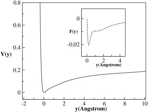
Figure 1: The effective potential felt by the tagged base pair in a dsDNA molecule (A18 of [4]) of 29 base pairs at separation $y$ at $45^{o}C$. In the inset the drift force $F(y)=-{\partial V(y)/\partial y}$ which drives the base pair to the equilibrium position is plotted.

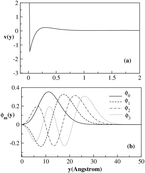
Figure 2: (a)The potential $v(y)$ of Eq.(6) at $45^{o}C$. The (repulsive) maximum in $v(y)$ corresponds to the minimum in the drift force $F(y)$. (b) Results of first few eigenfunctions as a function of $y$.

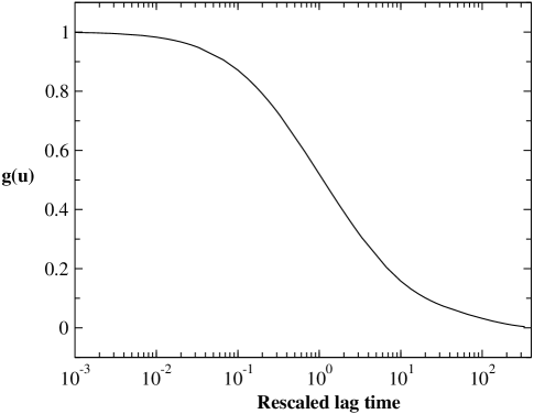
Figure 3: Rescaled autocorrelation function $g(u)=G(t/t_{1/2})$ where $G(t)=C(t)/C(0)$ and $t_{1/2}$ is such that $G(t_{1/2})=0.5$ as a function of $t/t_{1/2}$ at $45^{o}C$.These notations are same as used in [4].

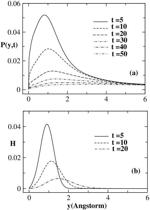
Figure 4: (a)Results for the distribution $P(y,t)$ as a function of separation $y$ at $45^{o}C$ for several time $t$ which are expressed in unit of $(\Gamma k_{B}Ta_{AT}^{2})^{-1}$. The peak in $P(y,t)$ represents the most probable separations. (b) Results for the half-time distribution $H(y,t/2|y^{\star},t;y^{\star},t=0)$ as a function of separation $y$ for $t=5,10,20$ for which $y^{\star}=0.84,1.01,1.24$. The peak in $H$ is found at separation larger than the corresponding value of $y^{\star}$.

References

- (1) W. Saenger, Principle of Nucleic Acid Structure (Springer Verlag, Berlin,1984).
- (2) J. Sontalucia Jr., Proc Nat. Acad. Sci., U.S.A. 95, 1460 (1998); F.Pincet, E. Perez, G. Bryant et al., Phys. Rev. Lett. 73, 2780 (1994); A. Krueger, E. Protozanova and M. D. Frank-Kamenetskii, Biophys. J. 90, 3091 (2006).
- (3) A. Campa, Phys. Rev. E 63, 021901 (2001), M. Peyrard, Europhys. Lett. 44, 271 (1998).
- (4) G. Altan-Bonnet, A. Libchaber and O. Krichevsky , Phys. Rev. Lett. 90, 138101 (2003).
- (5) M. Guéron, M. Kochoyan and J. L. Leroy, Nature (London) 328, 89 (1987).
- (6) R. M. Wartall and A. S. Benight, Phys. Rep. 126, 67 (1985).
- (7) A. Kornberg and T. A. Baker, DNA Replication (W. H. Freeman, NewYork, 1992).
- (8) R. J. Robert and X. Chang, Annu. Rev. Biochem. 67, 181 (1998); J. T. Stivers, Nucleic Acid Res Mol. Biol. 77, 37 (2004); J. F. Léger et al., Proc Nat. Acad. Sci., U.S.A. 95, 12295(1998).
- (9) H. C. Fogedby and R. Metzler, Phys. Rev. Lett. 98, 070601 (2007);Phys. Rev. E 76, 061915 (2007).
- (10) D. Poland and H. A. Scheraga,Theory of Helix-Coil Transition in Biopolymers (Academic Press, New York,1970).
- (11) C. Vanderzande, Lattice Models of Polymers (Cambridge University Press, Cambridge, 1998)
- (12) D. J. Bicout and E. Kats, Phys. Rev. E 70, 010902(R) (2004).
- (13) T. Ambjörnsson et al., Phys. Rev. Lett. 97, 128105 (2006); Biophys. J. 92, 2674 (2007).
- (14) M. Peyrard and A. R. Bishop, Phys. Rev. Lett. 62, 2755 (1989); T. Dauxois, M. Peyrard and A. R. Bishop , Phys. Rev. E 47, 684 (1993).
- (15) A. Campa and A. Giansanti, Phys. Rev. E 58, 3585 (1998).
- (16) S. Cocco, R. Monasson and J. F. Marko, Proc. Natl. Acad., U.S.A. 98, 8608 (2001); Phys. Rev. E 65, 041907 (2002).
- (17) N. K. Voulgarakis et al., Phys. Rev. Lett. 96, 248101 (2006).
- (18) N. Singh and Y. Singh, Eur. Phys. J. E. 17, 7 (2005), 19, 233 (2006).
- (19) C. Tang, H. Nakanishi and J. S. Langer, Phys. Rev. A 40 ,995 (1989).
- (20) A. Sethia, S. Sanyal and Y. Singh, J. Chem. Phys. 93, 7268 (1990).