Noether symmetric $f(R)$ quantum cosmology and its classical correlations

Abstract

We quantize a flat FRW cosmology in the context of the $f(R)$ gravity by Noether symmetry approach. We explicitly calculate the form of $f(R)$ for which such symmetries exist. It is shown that the existence of a Noether symmetry yields a general solution of the Wheeler-DeWitt equation where can be expressed as a superposition of states of the form $e^{iS}$. In terms of Hartle criterion, this type of wave function exhibits classical correlations, i.e. the emergent of classical universe is expected due to the oscillating behavior of the solutions of Wheeler-DeWitt equation. According to this interpretation we also provide the Noether symmetric classical solutions of our $f(R)$ cosmological model.
PACS numbers: 98.80.Qc, 04.50.+h, 04.20.Fy

1 Introduction

In recent years, modified theories of gravity constructed by adding correction terms to the usual Einstein-Hilbert action, have opened a new window to study the accelerated expansion of the universe. It has been shown that such correction terms could give rise to accelerating solutions of the field equations without having to invoke concepts such as dark energy [1]. In a more general setting, one can use a generic function $f(R)$, instead of the usual Ricci scalar $R$ as the action of general relativity. Such $f(R)$ gravity theories have been extensively studied in the literature over the past few years, see [2] for a review. In finding the dynamical equations of motion one can vary the action with respect to the metric (metric formalism), or view the metric and connections as independent dynamical variables and vary the action with respect to both independently (Palatini formalism) [3]. In this theory, the Palatini form of the action is shown to be equivalent to a scalar-tensor type theory from which the scalar field kinetic energy is absent. This is achieved by introducing a conformal transformation in which the conformal factor is taken as an auxiliary scalar field [4]. As is well known, in the usual Einstein-Hilbert action these two approaches give the same field equations. However, in $f(R)$ gravity the Palatini formalism leads to different dynamical equations due to nonlinear terms in the action. There is also a third version of $f(R)$ gravity in which the Lagrangian of the matter depends on the connections of the metric (metric-affine formalism) [5].

In a previous work [6], we studied a flat FRW space-time in the framework of the metric formalism of $f(R)$ gravity. In [6] we constructed an effective Lagrangian in the minisuperspace $\{a,R\}$ where $a$ and $R$ being the scale factor and Ricci scalar respectively. The form of the function $f(R)$ appearing in the modified action is then found by demanding that the Lagrangian admits the desired Noether symmetry [7]. A similar study of this issue in the Palatini framework can be found in [8]. By the Noether symmetry of a given minisuperspace cosmological model we mean that there exists a vector field $X$, as the infinitesimal generator of the symmetry on the tangent space of the configuration space such that the Lie derivative of the Lagrangian with respect to this vector field vanishes. For some applications of the Noether symmetry approach in various cosmological models see [9].

As mentioned above, although the corrections to the results of standard general relativity are widely investigated in literature in the $f(R)$ gravity context, these works are often in the classical regimes [10]. The cases dealing with quantum $f(R)$ models have seldom been studied in the literature [11], and it would be of interest to employ such models in this study.

In this paper we consider the same model as in [6] and try to quantize it by Noether symmetry approach. In general, the existence of a symmetry results in appearing of constants of motion which are related to the existence of cyclic variables in the dynamics [12]. This is the key result in our quantization procedure. Indeed, in terms of the cyclic variables the conserved quantities are nothing but the corresponding conjugate momenta. We shall see that applying the quantum version of these symmetries on the wave function of the universe (which satisfies the Wheeler-DeWitt equation) yields an oscillatory behavior for the wave function in the direction of the symmetries. On the other hand, in the semiclassical approximation for the canonical quantum gravity, one can show that a wave function with classical correlations is a superposition of states of the form $e^{iS}$, i.e. with oscillatory behavior [13]. With this interpretation scheme for the solutions of Wheeler-DeWitt equation, we also obtain the classical trajectory and show that the cosmological scale factor obeys a power law expansion.

It is to be noted that our presentation of quantum cosmology is applying quantum mechanics to a reduced dynamical system, the so-called minisuperspace. This is because that the fundamental equation of quantum cosmology, the Wheeler-DeWitt equation, is a differential equation on the infinite dimensional superspace and dealing with its solutions in such a space is not an easy task. Therefore, in order to solve this equation and obtain the wave function of the universe we can use an approximation method in which one truncates the infinite degrees of freedom to a finite dimensional submanifold called minisuperspace. In an alternative approach to deal with quantum effects in the early universe one can use the idea of quantum field theory in curved space time [14]. In this theory we assume that the matter fields are quantized while the gravitational field is classical and given by Einstein or any other modified gravity field equations. In this scheme quantum gravity is truncated at one-loop level and for computation of the one-loop corrections quantum fluctuations are imposed on a given classical background. Our aim in this letter is to study of quantization procedure in a Noether symmetric $f(R)$ gravity model in a reduced phase space framework, i.e. as mentioned above we first fix the background and then try to quantize it by Wheeler-DeWitt approach. In [15] the role of quantum effects to the background cosmology at one-loop level are investigated in $f(R)$ gravity framework.

2 The Noether symmetric phase space of the model

In this section we consider a spatially flat FRW cosmology within the framework of $f(R)$ gravity. Since our goal is to study models which exhibit Noether symmetry, we do not include any matter contribution in the action. Let us start from the action (we work in units where $c=\hbar=16\pi G=1$)

$${\cal S}=\int d^{4}x\sqrt{-g}f(R),$$ (1)

where $R$ is the scalar curvature and $f(R)$ is an arbitrary function of $R$. By varying the above action with respect to metric we obtain the equation of motion as

$$\frac{1}{2}g_{\mu\nu}f(R)-R_{\mu\nu}f^{\prime}(R)+\nabla_{\mu}\nabla_{\nu}f^{\prime}(R)-g_{\mu\nu}\Box f^{\prime}(R)=0,$$ (2)

where a prime represents differentiation with respect to $R$. We assume that the geometry of space-time is described by the flat FRW metric which seems to be consistent with the present cosmological observations

$$ds^{2}=-dt^{2}+a^{2}(t)\sum_{i=1}^{3}(dx^{i})^{2}.$$ (3)

With this background geometry the field equations read

$$2\dot{H}+3H^{2}=-\frac{1}{f^{\prime}}\left[f^{\prime\prime\prime}\dot{R}^{2}+2H\dot{R}f^{\prime\prime}+f^{\prime\prime}\ddot{R}+\frac{1}{2}(f-Rf^{\prime})\right],$$ (4)

$$H^{2}=\frac{1}{6f^{\prime}}\left[(f^{\prime}R-f)-6\dot{R}Hf^{\prime\prime}\right],$$ (5)

where $H=\dot{a}/a$ is the Hubble parameter and a dot represents differentiation with respect to $t$. To study the symmetries of the minisuperspace under consideration, we need an effective point-like Lagrangian for the model whose variation with respect to its dynamical variables yields the correct equations of motion. Following [16], we consider the action described above as representing a dynamical system in which the scale factor $a$ and scalar curvature $R$ play the role of independent dynamical variables. In [6, 12, 16] it is shown that such point-like Lagrangian takes the form

$${\cal L}(a,\dot{a},R,\dot{R})=6\dot{a}^{2}af^{\prime}+6\dot{a}\dot{R}a^{2}f^{\prime\prime}+a^{3}(f^{\prime}R-f).$$ (6)

The Hamiltonian corresponding to Lagrangian (6) can then be written in terms of $a$, $\dot{a}$, $R$ and $\dot{R}$ as

$${\cal H}(a,\dot{a},R,\dot{R})=6\dot{a}^{2}af^{\prime}+6\dot{a}\dot{R}a^{2}f^{\prime\prime}-a^{3}(f^{\prime}R-f).$$ (7)

Therefore, our cosmological setting is equivalent to a dynamical system where the phase space is spanned by $\left\{a,R,p_{a},p_{R}\right\}$ with Lagrangian (6) describing the dynamics with respect to time $t$. Now, it is easy to see that variation of Lagrangian (6) with respect to $R$ gives the well-known relation for the scalar curvature, while variation with respect to $a$ yields the field equation (4). Also, equation (5) is nothing but the zero energy condition ${\cal H}=0$ (Hamiltonian constraint).

As is well known, Noether symmetry approach is a powerful tool in finding the solution to a given Lagrangian, including the one presented above. In this approach, one is concerned with finding the cyclic variables related to conserved quantities and consequently reducing the dynamics of the system to a manageable one. The investigation of Noether symmetry in the model presented above is therefore the goal we shall pursue here. Following [7], we define the Noether symmetry induced on the model by a vector field $X$ on the tangent space $TQ=\left(a,R,\dot{a},\dot{R}\right)$ of the configuration space $Q=\left(a,R\right)$ of Lagrangian (6) as

$$X=\alpha\frac{\partial}{\partial a}+\beta\frac{\partial}{\partial R}+\frac{d\alpha}{dt}\frac{\partial}{\partial\dot{a}}+\frac{d\beta}{dt}\frac{\partial}{\partial\dot{R}},$$ (8)

such that the Lie derivative of the Lagrangian with respect to this vector field vanishes

$$L_{X}{\cal L}=0.$$ (9)

In (8), $\alpha$ and $\beta$ are some unknown functions of $a$ and $R$. Now, it is easy to see that the constants of motion corresponding to such a symmetry are [6, 12]

$$Q=\alpha p_{a}+\beta p_{R}.$$ (10)

In order to obtain the functions $\alpha$ and $\beta$ we use equation (9). In general this equation gives a quadratic polynomial in terms of $\dot{a}$ and $\dot{R}$ with coefficients being partial derivatives of $\alpha$ and $\beta$ with respect to the configuration variables $a$ and $R$. Thus, the resulting expression is identically equal to zero if and only if these coefficients are zero. This leads to a system of partial differential equations for $\alpha$ and $\beta$ [6]-[9]. For the model at hand, this system of differential equations has been investigated carefully in [6] and it has been shown that in the case where $f^{\prime\prime}\neq 0$, we have the following solutions

$$\alpha(a)=-\frac{1}{2}a^{-1},\hskip 14.22636pt\beta(a,R)=Ra^{-2},$$ (11)

and

$$f(R)=R^{\frac{3}{2}}.$$ (12)

Substituting this results into equation (6) we obtain the Lagrangian of the Noether symmetric model as

$${\cal L}=9\dot{a}^{2}aR^{1/2}+\frac{9}{2}\dot{a}\dot{R}a^{2}R^{-1/2}+\frac{1}{2}a^{3}R^{3/2}.$$ (13)

The momenta conjugate to variables $a$ and $R$ are

$$p_{a}=\frac{\partial{\cal L}}{\partial\dot{a}}=18\dot{a}aR^{1/2}+\frac{9}{2}a^{2}\dot{R}R^{-1/2},$$ (14)

$$p_{R}=\frac{\partial{\cal L}}{\partial\dot{R}}=\frac{9}{2}\dot{a}a^{2}R^{-1/2}.$$ (15)

Therefore, the corresponding Hamiltonian reads

$${\cal H}=\frac{2}{9}a^{-2}R^{1/2}p_{a}p_{R}-\frac{4}{9}a^{-3}R^{3/2}p_{R}^{2}-\frac{1}{2}a^{3}R^{3/2}.$$ (16)

Although, the classical equations of motion resulting from the Lagrangian (13) or Hamiltonian (16) can be solved to give the corresponding classical cosmology, Hamiltonian (16) has not the desired form for the construction of the Wheeler-DeWitt equation describing the relevant quantum cosmology. Furthermore, the Lagrangian (13) does not exhibit the existence of a cyclic variable corresponded to the Noether symmetry. To be more precise, we seek a point transformation $(a,R)\rightarrow(u,v)$ on the vector field (8) such that in terms of the new variables $(u,v)$, the Lagrangian includes one cyclic variable. A general discussion of this issue can be found in [12]. Under such point transformation it is easy to show that the vector field (8) takes the form

$$\tilde{X}=(Xu)\frac{\partial}{\partial u}+(Xv)\frac{\partial}{\partial v}+\frac{d}{dt}(Xu)\frac{\partial}{\partial\dot{u}}+\frac{d}{dt}(Xv)\frac{\partial}{\partial\dot{v}}.$$ (17)

One can show that if $X$ is a Noether symmetry of the Lagrangian, $\tilde{X}$ has also this property, that is

$$X{\cal L}=0\Rightarrow\tilde{X}{\cal L}=0.$$ (18)

Thus, if we demand

$$Xu=1,\hskip 14.22636ptXv=0,$$ (19)

we get

$$\tilde{X}=\frac{\partial}{\partial u}\Rightarrow\tilde{X}{\cal L}=\frac{\partial{\cal L}}{\partial u}=0.$$ (20)

This means that $u$ is a cyclic variable and the dynamics can be reduced. On the other hand, the constant of motion $Q$ becomes

$$Q=\alpha p_{a}+\beta p_{R}=\alpha\frac{\partial{\cal L}}{\partial\dot{a}}+\beta\frac{\partial{\cal L}}{\partial\dot{R}}=$$

$$\alpha\left(\frac{\partial{\cal L}}{\partial u}\frac{\partial u}{\partial\dot{a}}+\frac{\partial{\cal L}}{\partial v}\frac{\partial v}{\partial\dot{a}}+\frac{\partial{\cal L}}{\partial\dot{u}}\frac{\partial\dot{u}}{\partial\dot{a}}+\frac{\partial{\cal L}}{\partial\dot{v}}\frac{\partial\dot{v}}{\partial\dot{a}}\right)+\beta\left(\frac{\partial{\cal L}}{\partial u}\frac{\partial u}{\partial\dot{R}}+\frac{\partial{\cal L}}{\partial v}\frac{\partial v}{\partial\dot{R}}+\frac{\partial{\cal L}}{\partial\dot{u}}\frac{\partial\dot{u}}{\partial\dot{R}}+\frac{\partial{\cal L}}{\partial\dot{v}}\frac{\partial\dot{v}}{\partial\dot{R}}\right).$$ (21)

Since $(a,R)\rightarrow(u,v)$ is a point transformation, we have

$$\frac{\partial u}{\partial\dot{a}}=\frac{\partial v}{\partial\dot{a}}=\frac{\partial u}{\partial\dot{R}}=\frac{\partial v}{\partial\dot{R}}=0,$$

and

$$\frac{\partial\dot{u}}{\partial\dot{a}}=\frac{\partial u}{\partial a},\hskip 14.22636pt\frac{\partial\dot{u}}{\partial\dot{R}}=\frac{\partial u}{\partial R},\hskip 14.22636pt\frac{\partial\dot{v}}{\partial\dot{a}}=\frac{\partial v}{\partial a},\hskip 14.22636pt\frac{\partial\dot{u}}{\partial\dot{R}}=\frac{\partial v}{\partial R}.$$

Therefore,

$$Q=\alpha\left(\frac{\partial{\cal L}}{\partial\dot{u}}\frac{\partial u}{\partial a}+\frac{\partial{\cal L}}{\partial\dot{v}}\frac{\partial v}{\partial a}\right)+\beta\left(\frac{\partial{\cal L}}{\partial\dot{u}}\frac{\partial u}{\partial R}+\frac{\partial{\cal L}}{\partial\dot{v}}\frac{\partial v}{\partial R}\right)=$$

$$\left(\alpha\frac{\partial u}{\partial a}+\beta\frac{\partial u}{\partial R}\right)\frac{\partial{\cal L}}{\partial\dot{u}}+\left(\alpha\frac{\partial v}{\partial a}+\beta\frac{\partial v}{\partial R}\right)\frac{\partial{\cal L}}{\partial\dot{v}}=$$

$$(Xu)\frac{\partial{\cal L}}{\partial\dot{u}}+(Xv)\frac{\partial{\cal L}}{\partial\dot{v}}=\frac{\partial{\cal L}}{\partial\dot{u}}=p_{u}.$$ (22)

Thus, as expected the constant of motion which corresponds to the Noether symmetry is nothing but the momentum conjugated to the cyclic variable. To find the explicit form of the above mentioned point transformation we should solve the equations (19), which give

$$-\frac{1}{2}a^{-1}\frac{\partial u}{\partial a}+Ra^{-2}\frac{\partial u}{\partial R}=1,$$ (23)

$$-\frac{1}{2}a^{-1}\frac{\partial v}{\partial a}+Ra^{-2}\frac{\partial v}{\partial R}=0.$$ (24)

These differential equations admit the following general solutions

$$u(a,R)=-a^{2}+\phi_{1}(aR^{1/2}),\hskip 14.22636ptv(a,R)=\phi_{2}(aR^{1/2}),$$ (25)

where $\phi_{1}$ and $\phi_{2}$ are two arbitrary functions of $aR^{1/2}$. As is indicated in [12], ”the change of coordinates is not unique and a clever choice is always important.” With a glance at the Lagrangian (13), we choose the functions $\phi_{1}$ and $\phi_{2}$ as

$$\phi_{1}(aR^{1/2})=(aR^{1/2})^{\mu},\hskip 14.22636pt\phi_{2}(aR^{1/2})=(aR^{1/2})^{\nu},$$ (26)

where $\mu$ and $\nu$ are some constants. With this choice, the Lagrangian (13) takes the form

$${\cal L}=\frac{9}{2}\frac{\mu}{\nu^{2}}v^{\frac{\mu-2\nu+1}{\nu}}\dot{v}^{2}-\frac{9}{2\nu}v^{\frac{1-\nu}{\nu}}\dot{u}\dot{v}+\frac{1}{2}v^{3/\nu}.$$ (27)

It is clear from this Lagrangian that $u$ is cyclic and the Noether symmetry is given by $p_{u}=Q=\mbox{cons.}$. Also, the momenta conjugate to $u$ and $v$ are

$$p_{u}=\frac{\partial{\cal L}}{\partial\dot{u}}=-\frac{9}{2\nu}v^{\frac{1-\nu}{\nu}}\dot{v},\hskip 14.22636ptp_{v}=\frac{\partial{\cal L}}{\partial\dot{v}}=9\frac{\mu}{\nu^{2}}v^{\frac{\mu-2\nu+1}{\nu}}\dot{v}-\frac{9}{2\nu}v^{\frac{1-\nu}{\nu}}\dot{u},$$ (28)

which give rise to the following Hamiltonian for our dynamical system

$${\cal H}=-\frac{10}{9}\mu v^{\frac{\mu-1}{\nu}}p_{u}^{2}-\frac{2}{3}\nu v^{\frac{\nu-1}{\nu}}p_{u}p_{v}-\frac{1}{2}v^{3/\nu}.$$ (29)

The preliminary set-up for writing the action is now complete. In the next section, we shall focus attention on the study of the quantum cosmology of the model described above.

3 Quantization of the model

Standard cosmological models based on classical general relativity have no convincing precise answer for the presence of the so-called Big-Bang singularity. Any hope of dealing with such singularities would be in vein unless a reliable quantum theory of gravity can be constructed. In the absence of a full theory of quantum gravity, it would be useful to describe the quantum states of the universe within the context of quantum cosmology [20]. In this formalism which is based on the canonical quantization procedure, one first freezes a large number of degrees of freedom and then quantizes the remaining ones. The quantum state of the universe is then described by a wave function in the minisuperspace, a function of the 3-geometry of the model and matter fields presented in the theory, satisfying the Wheeler-DeWitt equation, that is, ${\cal H}\Psi=0$, where ${\cal H}$ is the operator form of the Hamiltonian given by equation (29) and $\Psi$ is the wave function of the universe. On the other hand, the existence of a Noether symmetry in the model reduces the dynamics through $p_{u}=Q$, where its quantum version can be considered as a constraint $p_{u}\Psi=Q\Psi$. Therefore, the quantum cosmology of our Noether symmetric $f(R)$ model can be described by the following equations

$${\cal H}\Psi(u,v)=\left[-\frac{10}{9}\mu v^{\frac{\mu-1}{\nu}}p_{u}^{2}-\frac{1}{3}\nu\left(v^{r}p_{v}v^{s}+v^{s}p_{v}v^{r}\right)p_{u}-\frac{1}{2}v^{3/\nu}\right]\Psi(u,v)=0,$$ (30)

$$p_{u}\Psi(u,v)=Q\Psi(u,v),$$ (31)

where the parameters $r$ and $s$ satisfy $r+s=\frac{\nu-1}{\nu}$ and denote the ambiguity in the ordering of factors $v$ and $p_{v}$ in the second term of (29). With the replacement $p_{u}\rightarrow-i\frac{\partial}{\partial u}$ and similarly for $p_{v}$ the above equations read

$$\left[\frac{10}{9}\mu v^{\frac{\mu-1}{\nu}}\frac{\partial^{2}}{\partial u^{2}}+\frac{\nu-1}{3}v^{-1/\nu}\frac{\partial}{\partial u}+\frac{2}{3}\nu v^{\frac{\nu-1}{\nu}}\frac{\partial^{2}}{\partial u\partial v}-\frac{1}{2}v^{3/\nu}\right]\Psi(u,v)=0,$$ (32)

$$-i\frac{\partial}{\partial u}\Psi(u,v)=Q\Psi(u,v).$$ (33)

The solutions of the above differential equations are separable and may be written in the form $\Psi(u,v)=U(u)V(v)$. Equation (33) can be immediately integrated leading to a oscillatory behavior for the wave function in $u$ direction, i.e. in the direction of symmetry, that is

$$\Psi(u,v)=e^{iQu}V(v).$$ (34)

Substitution this result into relation (32) yields the following equation for the function $V(v)$

$$\frac{dV}{dv}=\left[-\frac{5}{3}i\frac{\mu}{\nu}Qv^{\frac{\mu-\nu}{\nu}}-\frac{3}{4\nu Q}iv^{\frac{4-\nu}{\nu}}-\frac{\nu-1}{2\nu}v^{-1}\right]V(v),$$ (35)

with solution

$$V(v)=v^{\frac{1-\nu}{2\nu}}e^{-i\left(\frac{5}{3}Qv^{\mu/\nu}+\frac{3}{16Q}v^{4/\nu}\right)}.$$ (36)

Thus, the eigenfunctions of the equations (32) and (33) can be written as

$$\Psi_{\mu\nu}(u,v)=v^{\frac{1-\nu}{2\nu}}e^{i\left(Qu-\frac{5}{3}Qv^{\mu/\nu}-\frac{3}{16Q}v^{4/\nu}\right)}.$$ (37)

We may now write the general solutions to the Wheeler-DeWitt equation as a superposition of the eigenfunctions with shifted Gaussian weight functions

$$\Psi(u,v)=\int_{-\infty}^{+\infty}\int_{-\infty}^{+\infty}e^{-\varsigma(\mu-\mu_{0})^{2}}e^{-\sigma(\nu-\nu_{0})^{2}}v^{\frac{1-\nu}{2\nu}}e^{i\left(Qu-\frac{5}{3}Qv^{\mu/\nu}-\frac{3}{16Q}v^{4/\nu}\right)}d\mu d\nu.$$ (38)

We see that the wave function is a superposition of states of the form $e^{iS}$. In semiclassical approximation for quantum gravity [13], this type of state represents the correlations between classical trajectories and the peaks of the wave function [12]. Inserting $\Psi\sim e^{iS}$ into Wheeler-DeWitt equation, we are led to the Hamilton-Jacobi equation for $S$. Thus, the classical trajectories can be obtained by rewriting the momenta as derivative of $S$ with respect to the corresponding variables, that is, $p_{q}=\frac{\partial S}{\partial q}$. Therefore, in semiclassical limit, by identifying the exponential factor of (37) with $S$, we can recover the corresponding classical cosmology

$$S=Qu-\frac{5}{3}v^{\mu/\nu}-\frac{3}{16Q}v^{4/\nu}.$$ (39)

The classical trajectories, which determine the behavior of the scale factor and Ricci scalar are given by

$$p_{u}=\frac{\partial S}{\partial u},\hskip 14.22636ptp_{v}=\frac{\partial S}{\partial v}.$$

Using the definition of $p_{u}$ and $p_{v}$ in (28), the equations for the classical trajectories become

$$-\frac{9}{2\nu}v^{\frac{1-\nu}{\nu}}\dot{v}=Q,$$ (40)

$$9\frac{\mu}{\nu^{2}}v^{\frac{\mu-2\nu+1}{\nu}}\dot{v}-\frac{9}{2\nu}v^{\frac{1-\nu}{\nu}}\dot{u}=-\frac{5}{3}\frac{\mu}{\nu}Qv^{\frac{\mu-\nu}{\nu}}-\frac{3}{4Q\nu}v^{\frac{4-\nu}{\nu}}.$$ (41)

Equation (40) can be easily integrated leading to

$$v(t)=\left({\cal Q}t-t_{0}\right)^{\nu},$$ (42)

where ${\cal Q}=-\frac{2}{9}Q$ and $t_{0}$ is an integrating constant. Substituting the above results into equation (41) yields

$$u(t)=\frac{1}{3}\left({\cal Q}t-t_{0}\right)^{\mu}-\frac{1}{108{\cal Q}^{2}}\left({\cal Q}t-t_{0}\right)^{4}+C,$$ (43)

where $C$ is another integrating constant which we can choose it to be zero. Going back to the variables $a$ and $R$, we obtain the corresponding classical cosmology as

$$a(t)=\left[\frac{2}{3}\left({\cal Q}t-t_{0}\right)^{\mu}+\frac{1}{108{\cal Q}^{2}}\left({\cal Q}t-t_{0}\right)^{4}\right]^{1/2},$$ (44)

$$R(t)=\frac{\left({\cal Q}t-t_{0}\right)^{2}}{\frac{2}{3}\left({\cal Q}t-t_{0}\right)^{\mu}+\frac{1}{108{\cal Q}^{2}}\left({\cal Q}t-t_{0}\right)^{4}}.$$ (45)

For $t\rightarrow t_{0}/{\cal Q}$, we have an initial singularity in which the scale factor goes to zero while the Ricci scalar has a large value. On the other hand, in the late time, the universe evolves with a power law expansion ($a(t)\sim t^{2}$ for $0<\mu\leq 4$ and $a(t)\sim t^{\mu/2}$ for $\mu>4$) and the scalar curvature goes to zero in this limit.

In general, one of the most important features in quantum cosmology is the recovery of classical cosmology from the corresponding quantum model, or in other words, how can the Wheeler-DeWitt wave functions predict a classical universe. We see that the oscillatory solutions of the form $\Psi\sim e^{iS}$ for Wheeler-DeWitt equation yield the classical solution (44) which for positive values of $\mu$ can be viewed as an accelerating cosmology. Since the quantum effects in cosmology are important in the very early times of cosmic evolution, we immediately see that, in this limit, the scale factor has the behavior $a(t)\sim t^{\mu/2}$ for $0<\mu\leq 4$ and $a(t)\sim t^{2}$ for $\mu>4$, which for $\mu>2$ describe a power law inflationary behavior. The universe then undergoes to a late-time accelerating phase, also with a power law expansion behavior. An important question in inflationary models is how much inflation do the model predict or in other words, what is the mechanism through which the universe exits from the inflationary epoch and undergoes into radiation or matter-dominated eras. As is well known, this is largely depend on the behavior of a scalar field with which the universe nucleates [21]. In $f(R)$ gravity models some of such mechanisms describing the transition between different epochs of cosmic evolution are proposed in [22] by introducing a scalar field $\phi$. Indeed, it is easy to verify that the metric $f(R)$ gravity action (1) is dynamically equivalent to [2]

$${\cal S}=\int d^{4}x\sqrt{-g}\left[\phi R-V(\phi)\right],$$ (46)

where $\phi=f^{\prime}(R)$ and $V(\phi)=\phi R(\phi)-f(R(\phi))$. In our $f(R)\sim R^{3/2}$ model we have $R(\phi)\sim\phi^{2}$ and hence $V(\phi)\sim\phi^{3}$. The dynamics of this scalar field may show the the possibility of the transition between different eras of cosmic evolution. But as is indicated in [22] ”we should note that in this case, there is no matter and $f(R)$-terms contribution plays the role of the matter instead of the real matter”. Therefore, it is to be noted that our presentation does not claim to clear the role of inflation scenario in a fundamental way because we just study the problem in a special simple model. However, this may reflect realistic scenarios in similar investigations which deal with this problem in a more fundamental way [22].

From equations (42) and (43) we see that the classical trajectories obey the relation

$$u=\frac{1}{3}v^{\mu/\nu}-\frac{1}{108{\cal Q}^{2}}v^{4/\nu}.$$ (47)

As we have mentioned above (see (38)), we are looking for a coherent wave function with a good asymptotic behavior in the minisuperspace and peaking in the vicinity of the classical loci (47) in the configuration space spanned by $\{u,v\}$. It is well known that the general solution of Wheeler-DeWitt equation may be constructed by superposition of its eigenfunctions which in our problem at hand are labeled by $\mu$ and $\nu$. Therefore, the wavepacket (38) is what we need. We take the solution as being represented by equation (38) with the integrals to be truncated at suitable values of $\mu$ and $\nu$ displaying this peak. Figure 1 shows the square of wave function for typical values of the parameters where we have taken the integrals from 0 to 2 for $\mu$ and from -15 to 15 for $\nu$. It is seen that almost a good correlation exists between this pattern and the classical trajectories.

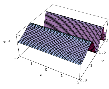
Figure 1: The square of wave function. The figure is plotted for numerical values $\varsigma=10$, $\sigma=5$, $\mu_{0}=3$, $\nu_{0}=0$ and $Q=3$.

4 Conclusions

In this letter we have studied a generic $f(R)$ cosmological model by Noether symmetry approach. For the background geometry, we have considered a flat FRW metric and derived the general equations of motion in this background. The phase space was then constructed by taking the scale factor $a$ and Ricci scalar $R$ as the independent dynamical variables. The Lagrangian of the model in the configuration space spanned by $\left\{a,R\right\}$ is so constructed such that its variation with respect to these dynamical variables yields the correct field equations. The existence of Noether symmetry implies that the Lie derivative of this Lagrangian with respect to the infinitesimal generator of the desired symmetry vanishes. In [6] we have shown that by applying this condition to the Lagrangian of the model, one can obtain the explicit form of the corresponding $f(R)$ function which has led us to the Lagrangian (13) and Hamiltonian (16) of the Noether symmetric model. Since the Lagrangian (13) does not exhibit the existence of a cyclic variable corresponded to the Noether symmetry, we have provided a point transformation $(a,R)\rightarrow(u,v)$ such that in terms of the new variables $(u,v)$, the Lagrangian includes one cyclic variable. We have then quantized the model and shown that the corresponding quantum cosmology and the ensuing Wheeler-DeWitt equation are amenable to exact solutions in terms of a superposition of states of the form $e^{iS}$ due to the existence of Noether symmetry. In semiclassical approximation for quantum gravity, this type of state represents the correlations between classical trajectories and the peaks of the wave function. Using this interpretation we have shown that the corresponding classical cosmology results in a power law accelerated expansion for the scale factor of the universe either in its early or late time evolution.

References

-
[1]
C. Deffayet, Phys. Lett. B 502 (2001) 199
(arXiv: hep-th/0010186)
J.S. Alcaniz, Phys. Rev. D 65 (2002) 123514 (arXiv: astro-ph/0202492)
S.M. Carroll, V. Duvvuri, M. Trodden and M. Turner, Phys. Rev. D 70 (2004) 043528 (arXiv: astro-ph/0306438)
S. Nojiri and S.D. Odintsov, Phys. Lett. B 576 (2003) 5 (arXiv: hep-th/0307071)
K. Atazadeh and H.R. Sepangi, Int. J. Mod. Phys. D 16 (2007) 687 (arXiv: gr-qc/0602028)
S. Nojiri, S.D. Odintsov and M. Sami, Phys. Rev. D 74 (2006) 046004 (arXiv: hep-th/0605039)
S. Capozziello and M. Francaviglia, Gen. Rel. Grav. 40 (2008) 357
S. Capozziello, Int. J. Mod. Phys. D 11 (2002) 483 (arXiv: gr-qc/0201033)
S. Capozziello, S. Carloni and A. Troisi, Recent Research Developments in Astronomy and Astrophysics RSP/AA/21-2003 (arXiv: astro-ph/0303041)
S. Nojiri and S. D. Odintsov, Phys.Rev. D 68 (2003) 123512 (arXiv:hep-th/0307288)
S. Nojiri and S.D. Odintsov, Can F(R)-gravity be a viable model: the universal unification scenario for inflation, dark energy and dark matter (arXiv: 0801.4843 [astro-ph]) -
[2]
S. Nojiri and S.D. Odintsov, Dark energy, inflation and dark matter from modified
gravity (arXiv: 0807.0685 [hep-th])
S. Nojiri and S.D. Odintsov, Int. J. Geom. Methods Mod. Phys. 4 (2007) 115 (arXiv: hep-th/ 0601213)
T.P. Sotiriou and V. Faraoni, theories of gravity (arXiv: 0805.1726 [gr-qc]) -
[3]
D.N. Vollick, Phys. Rev. D 68 (2003)
063510 (arXiv: astro-ph/0306630)
X. Meng and P. Wang, Class. Quantum Grav. 20 (2003) 4949 (arXiv: astro-ph/0307354)
X. Meng and P. Wang, Palatini formulation of modified gravity with squared scalar curvature (arXiv: astro-ph/0308284)
X. Meng and P. Wang, Phys. Lett. B 584 (2004) 1 (arXiv: hep-th/0309062) -
[4]
E.E. Flanagan, Class. Quantum Grav. 21
(2003) 417 (arXiv: gr-qc/0309015)
E.E. Flanagan, Phys. Rev. Lett. 92 (2004) 071101 (arXix: astro-ph/0308111)
G. Magnano, L.M. Sokolowski, Phys.Rev. D 50 (1994) 5039 (arXiv: gr-qc/9312008) -
[5]
T.P. Sotiriou and S. Liberati, Ann. Phys. 322 (2007) 935 (arXiv: gr-qc/0604006)
N.J. Poplawski, Class. Quantum Grav. 23 (2006) 2011 (arXiv: gr-qc/0510007) - [6] B. Vakili, Phys. Lett. B 664 (2008) 16 (arXiv: 0804.3449 [gr-qc])
-
[7]
M. Demianski, R. de Ritis, C. Rubano and P. Scudellaro, Phys. Rev. D 46 (1992)
1391
S. Capozziello, G. Marmo, C. Rubano and P. Scudellaro, Int. J. Mod. Phys. D 6 (1997) 491 (arXiv: gr-qc/9606050)
S. Capozziello, S. Nesseris and L. Perivolaropoulos, J. Cosmol. Astropart. Phys. JCAP 0712 (2007) 009 (arXiv:0705.3586 [astro-ph])
S. Capozziello and A. De Felice, cosmology by Noether’s symmetry (arXiv: 0804.2163 [gr-qc]) - [8] M. Roshan and F. Shojai, Palatini cosmology and Noether symmetry (arXiv: 0809.1272 [gr-qc])
-
[9]
S. Capozziello, V.I. Man’ko, G. Marmo and C.
Stornaiolo, Tomographic Representation of Minisuperspace
Quantum Cosmology and Noether Symmetries (arXiv: 0706.3018
[gr-qc])
S. Capozziello, A. Stabile and A. Troisi, Class. Quantum Grav. 24 (2007) 2153 (arXiv: gr-qc/0703067)
A.K. Sanyal, B. Modak, C. Rubano and E. Piedipalumbo, Gen. Rel. Grav. 37 (2005) 407 (arXiv: astro-ph/0310610)
A.K. Sanyal, Phys. Lett. B 524 (2002) 177 (arXiv: gr-qc/0107053)
A. K. Sanyal and B.M. Modak, Class. Quantum Grav. 18 (2001) 3767 (arXiv: gr-qc/0107052)
A. Bonanno, G. Esposito, C. Rubano and P. Scudellaro, Gen. Rel. Grav. 39 (2007) 189 (arXiv: astro-ph/0612091)
B. Vakili, N. Khosravi and H.R. Sepangi, Class. Quantum Grav. 24 (2007) 931 (arXiv: gr-qc/0701075)
H. Motavali, S. Capozziello and M.R. Almeh Jog, Scalar-tensor cosmology with curvature correction by Noether Symmetry (arXiv: 0807.0347 [gr-qc]) -
[10]
M.C.B. Abdalla, A. Nojiri and S.D. Odintsov, Class. Quantum Grav. 22 (2005) L35 (arXiv: hep-th/0409177)
X. Meng and P. Wang,Class. Quantum Grav. 22 (2005) 23 ( arXiv: gr-qc/0411007)
X. Meng and P. Wang, Class. Quantum Grav. 21 (2004) 951 (arXiv: astro-ph/0308031)
T. Clifton and J.D. Barrow, Phys. Rev. D 72 (2005) 103005 (arXiv: gr-qc/0509059)
T. Clifton, Class. Quantum Grav. 23 (2006) 7445 ( arXiv: gr-qc/0607096)
J.D. Barrow and T. Clifton, Class.Quantum Grav. 23 (2006) L1 ( arXiv: gr-qc/0509085) -
[11]
A. Shojai and F. Shojai, Gen. Rel. Grav. 40 (2008) 1967 (arXiv: 0801.3496 [gr-qc])
A.K. Sanyal and B. Modak, Phys. Rev. D 63 (2001) 064021 (arXiv: gr-qc/0107001)
A.K. Sanyal and B. Modak, Class.Quantum Grav. 19 (2002) 515 (arXiv: gr-qc/0107070) - [12] S. Capozziello and G. Lambiase, Gen. Rel. Grav. 32 (2000) 673 (arXiv: gr-qc/9912083)
-
[13]
G. Lifschytz, S.D. Mathur and M. Ortiz, Phys. Rev. D 53 (1996) 766 (arXiv: gr-qc/9412040)
J.J. Halliwell, Nucl. Phys. B 266 (1986) 228
J.J. Halliwell, Phys. Rev. D 36 (1987) 3626
J.B. Hartle, in Gravitation in Astrophysics, editors: S. Carter and J.B. Hartle (Plenum, New York 1986) -
[14]
N.D. Birell and P.C.W. Davies, Quantum Fields in Curved Space, Cambridge University Press, Cambridge, (1982)
B.R. Iyer, in Gravitation, Gauge Theories and the Early Universe, editors: B.R. Iyer, N. Mukunda and C.V. Vishveshwara, Kluwer Academic Publishers, (1988) -
[15]
G. Cognola et al., J. Cosmol. Astropart. Phys. JCAP 0502 (2005) 010 (arXiv: hep-th/0501096)
G. Cognola and S. Zerbini, J. Phys. A 39 (2006) 6245 (arXiv: hep-th/0511233) - [16] J.C.C. de Souza and V. Faraoni, Class. Quantum Grav. 24 (2007) 3637 (arXiv: 0706.1223 [gr-qc])
- [17] G. Cognola et al., Phys. Rev. D 77 (2008) 046009 (arXiv: 0712.4017 [hep-th])
-
[18]
W. Hu and I. Sawicki, Phys. Rev. D 76 (2007) 064004
(arXiv: 0705.1158 [astro-ph]
S. Nojiri and S.D. Odintsov, Newton law corrections and instabilities in gravity with the effective cosmological constant epoch (arXiv: 0706.1378 [hep-th])
S. Nojiri and S.D. Odintsov, (arXiv: 0707.1941 [hep-th])
S. Nojiri and S.D. Odintsov, Phys. Rev. D 77 (2008) 026007 (arXiv: 0710.1738 [hep-th]) - [19] T. Chiba, Phys. Lett. B 575 (2003) 1
-
[20]
B.S. DeWitt, Phys. Rev. 160 (1967) 1113
C.W. Misner, Phys. Rev. 186 (1969) 1319 - [21] A. Linde, in Inflationary Cosmology, editors: M. Lemoine, J. Martin and P. Peter (Springer, Lecture Notes in Physics 738, 2007)
-
[22]
S. Capozziello, S. Nojiri, S.D. Odintsov and A. Troisi, Phys. Lett. B 639 (2006) 135 (arXiv: astro-ph/0604431)
S. Nojiri and S.D. Odintsov, Phys. Rev. D 74 (2006) 086005 (arXiv: hep-th/0608008)