Hydrodynamics with conserved current from the gravity dual

Abstract:

We determine the structure of the hydrodynamics with conserved current, using the gauge/gravity duality of charged black-hole background. It turns out that even in the presence of the external electromagnetic field at the boundary, bulk Einstein equation is equivalent to the boundary conservation of energy momentum tensor and that of current. As a consequence, the thermal conductivity and electric conductivity are calculated in terms of the parameters of the fundamental theory. We find that Wiedermann-Franz law hold with Lorentz number $1/e^{2}$.

1 Introduction

After the discovery of consistency of AdS/CFT [1, 2, 3] and that of RHIC experiment on the viscosity/entropy-density ratio [4, 5, 6], much attention has been drawn to the calculational scheme provided by string theory. Some attempt has been made to map the entire process of RHIC experiment in terms of the gravity dual [7]. The way to include chemical potential in the theory was figured out in [8, 9] and phases of these theories were also discussed in D3/D7 setup [10, 11, 12, 9]. The essential feature is that the global U(1) charges in the boundary corresponds to the local U(1) charges in the bulk.

The gauge/gravity duality holds for the theory with $N=4$ Super Yang Mill system which is far from the real QCD. Therefore we need to search quantities which does not depends on the details of the theory like $\eta/s$. The hydrodynamics approach is especially useful in this respect since it is about dynamics of long wavelength and low frequency limit. Also, due to high temperature nature, all the fermions are decoupled.

Recently, in a very interesting paper [13], the authors showed that the hydrodynamic equation in the boundary theory is equivalent to the Einstein equation in the bulk. Usually the dissipative parts of the current and energy momentum tensor are constructed from the second law by considering the entropy current [14]. The method of reference [13] has the merit to determine the dissipative part of the energy momentum tensor without using the second law. This merit was applied to other different black holes [17, 18, 19, 20]. The purpose of this work is to determine the dissipative part of the conserved current along this line. We will also get transport coefficients in terms of the data of the Yang-Mill theory. Since the dual of the particle number can be regarded as the local charge of the Maxwell field in the bulk, we are lead to consider the charged black holes in AdS space. We consider only up to the first order in the derivative expansion. It turns out that our expression for the current is precisely agree with that of Landau-Lifshitz [14, 15]. The only difference is that the hydrodynamics transport coefficients are now determined from the fundamental theory.

The rest of the paper goes as follows: in section 2, we give an outline of calculational procedure following [13]. In section 3, we calculate the structure of conserved current using the perturbative solution to the first order in derivative expansion, which is enough to determine both thermal and electric conductivity. In section 4, we give a summary and discussion. In appendix, we list the important formula.

2 General construction

2.1 General procedure of calculation

In this section, we explain the general procedure of constructing solution. Our starting point is the Einstein Maxwell theory with a negative cosmological constant. The action is given by

$$S=\frac{1}{16\pi G}\int_{\mathcal{M}}d^{5}x\sqrt{-g}~{}\left[R+\frac{12}{l^{2}}\right] + \frac{1}{8\pi G}\int_{\partial\mathcal{M}}d^{4}x\sqrt{-\gamma}\Theta-\frac{1}{4g^{2}}\int_{\cal M}d^{5}x\sqrt{-g}F^{2}$$ (1)

$$+ \text{counter terms}~{}~{},$$

where the first and second terms are usual Einstein-Hilbert action and cosmological constant action, and third term is the Gibbons-Hawking term, where $\Theta$ is trace of extrinsic curvature $\Theta_{\mu\nu}$. Introducing spaces with boundary, this term should be added to the action. In addition, the counter terms are needed to cancel divergences of the action and boundary stress-energy tensor. This is well studied in [16]. Taking a unit, where $l=1$ and $16\pi G=1$, the equations of motion are given by

$$R_{IJ}-\frac{1}{2}g_{IJ}R-6g_{IJ}-\frac{1}{2g^{2}}\left(F_{IK}{F_{J}}^{K}-\frac{1}{4}g_{IJ}F^{2}\right)=0$$ (2)

$$\nabla_{J}{F^{J}}_{I}=0~{}~{}.$$ (3)

The solution we are interested in is the charged uniform black brane solution, which can be written as

$$ds^{2}=-r^{2}f(r)dv^{2}+2dvdr+r^{2}(dx_{1}^{2}+dx_{2}^{2}+dx_{3}^{2})$$ (4)

$$f(r)=1-\frac{2M}{r^{4}}+\frac{Q^{2}}{r^{6}}=\frac{(r^{2}-r_{+}^{2})(r^{2}-r_{-}^{2})(r^{2}+r_{+}^{2}+r_{-}^{2})}{r^{6}}$$

$$F=g\frac{2\sqrt{3}Q}{r^{3}}dv\wedge dr~{}~{}.$$

Here we use the Eddington-Finkelstein coordinate $v=t+r_{*}$ with $dr_{*}=dr/{f}$ to make the metric regular at the horizon $r_{+}$. It is slightly different from time coordinate ’$t$’. In the boosted frame, it can be written as

$$ds^{2}=-r^{2}f(r)(u_{\mu}dx^{\mu})^{2}-2u_{\mu}dx^{\mu}dr+r^{2}P_{\mu\nu}dx^{\mu}dx^{\nu}$$ (5)

$$F=-g\frac{2\sqrt{3}Q}{r^{3}}u_{\mu}dx^{\mu}\wedge dr~{}~{},~{}~{}A=\left(eA^{\rm ext}_{\mu}-\frac{\sqrt{3}gQ}{r^{2}}u_{\mu}\right)dx^{\mu}$$

$$u^{0}=\frac{1}{\sqrt{1-\beta_{i}^{2}}}~{}~{},~{}~{}u^{i}=\frac{\beta_{i}}{\sqrt{1-\beta_{i}^{2}}}$$

$$P_{\mu\nu}=\eta_{\mu\nu}+u_{\mu}u_{\nu}~{}~{},$$

where $M$, $Q$, $A^{\rm ext}_{\mu}$ and $\beta^{i}$’s are constants parametering solutions. It satisfies the equations of motion.

Now we lift above parameters to the functions of $x^{\mu}$. Then, (5) is not a solution of the equations of motion any more. To find make it a solution, we have to add corrections to it. To do this systematically, first we define following tensors

$$W_{IJ}=R_{IJ}+4g_{IJ}+\frac{1}{2g^{2}}\left(F_{IK}{F^{K}}_{J}+\frac{1}{6}g_{IJ}F^{2}\right)$$ (6)

$$W_{I}=\nabla_{J}{F^{J}}_{I}~{}~{}.$$ (7)

The equation of motion is given by the vanishing of $W_{IJ}$ and $W_{I}$. Taking parameters as functions of $x^{\mu}$ gives nonzero $W_{IJ}$ and $W_{I}$. By construction these are proportional to derivatives of parameter functions. We will call these terms by source terms. To cancel this source terms, we need to add some corrections to metric and gauge fields. We consider the derivative expansion and do it order by order. So obtaining new solution is reduced to finding these correction terms. Due to the redundancy in metric and gauge field, we can take a gauge choice for the correction terms. Our choice for $n$-th correction terms are

$${ds^{(n)}}^{2}=\frac{k_{n}(r)}{r^{2}}dv^{2}+2h_{n}(r)dvdr+2\frac{j^{i}_{n}(r)}{r^{2}}dvdx^{i}+r^{2}\left(\alpha^{n}_{ij}-\frac{2}{3}h_{n}(r)\delta_{ij}\right)dx^{i}dx^{j}$$ (8)

$$A^{(n)}=a^{n}_{v}(r)dv+a^{n}_{i}(r)dx^{i}~{}~{}.$$

For metric parts, this choice is the same as [13]. Since, for gauge field part, $a_{r}^{n}(r)$ does not contribute to field strength, the choice $a_{r}^{n}(r)=0$ is trivial.

Our procedure can be described as follows. First, we consider zeroth order solution. By construction, $S^{(0)}_{IJ}$ and $S^{(0)}_{J}$ are zero, and the zeroth order correction terms are also zero naturally. For the first order, we take the parameters in zeroth order solution as functions of $x^{\mu}$ and expand around $x^{\mu}=0$ up to first order in derivative. Putting these new metric and gauge fields into $W_{IJ}$ and $W_{I}$, we obtain the source terms $S^{(1)}_{IJ}=-W_{IJ}$ and $S^{(1)}_{I}=-W_{I}$. To make these source terms canceled, we consider correction terms in (8) for $n=1$, these make effects in $W_{IJ}$ and $W_{I}$. So $W_{IJ}=(\text{effect from correction})-S^{(1)}_{IJ}$ and $W_{I}=(\text{effect from correction})-S^{(1)}_{I}$, from this we can find corrections. Assuming we know $(n-1)$ th order solution, we can calculate $n$th derivative order source terms and we can obtain $n$th order correction terms in metric and gauge fields. For general $n$th order, in the Maxwell equation, what we have to do is just solving following equations

$$W_{v}=\frac{f(r)}{r}\left\{r^{3}{a^{n}_{v}}^{\prime}(r)+4\sqrt{3}gQh^{n}(r)\right\}^{\prime}-S^{(n)}_{v}(r)=0$$ (9)

$$W_{r}=-\frac{1}{r^{3}}\left\{r^{3}{a^{n}_{v}}^{\prime}(r)+4\sqrt{3}gQh^{n}(r)\right\}^{\prime}-S^{(n)}_{r}(r)=0$$

$$W_{i}=\frac{1}{r}\left\{r^{3}f(r){a^{n}_{i}}^{\prime}(r)-\frac{2\sqrt{3}gQ}{r^{4}}j^{i}_{n}(r)\right\}^{\prime}-S^{(n)}_{i}(r)=0~{}~{}.$$

For Einstein equations, the equations are

$$W_{vv}=f(r)\left\{\frac{4}{\sqrt{3}g}\frac{Q}{r}{a^{n}_{v}}^{\prime}(r)-8r^{2}h_{n}(r)-r^{2}(r^{2}f(r))^{\prime}{h_{n}}^{\prime}(r)-\frac{r}{2}\left(\frac{k^{\prime}_{n}(r)}{r}\right)^{\prime}\right\}-S^{(n)}_{vv}(r)=0$$

$$W_{vr}=8h_{n}(r)+(r^{2}f(r))^{\prime}h_{n}^{\prime}(r)-\frac{4}{\sqrt{3}g}\frac{Q}{r^{3}}{a^{n}_{v}}^{\prime}(r)+\frac{1}{2r}\left(\frac{k_{n}^{\prime}(r)}{r}\right)^{\prime}-S^{(n)}_{vr}(r)=0$$

$$W_{vi}=f(r)\left\{\frac{\sqrt{3}Q}{gr}{a^{n}_{i}}^{\prime}(r)-\frac{r^{3}}{2}\left(\frac{{j_{n}^{i}}^{\prime}(r)}{r^{3}}\right)^{\prime}\right\}-S^{(n)}_{vi}(r)=0$$

$$W_{rr}=\frac{1}{r^{5}}(r^{5}h_{n}^{\prime}(r))^{\prime}-S^{(n)}_{rr}(r)=0$$

$$W_{ri}=-\frac{\sqrt{3}Q}{gr^{3}}{a^{n}_{i}}^{\prime}(r)+\frac{r}{2}\left(\frac{{j_{n}^{i}}^{\prime}(r)}{r^{3}}\right)^{\prime}-S^{(n)}_{ri}(r)=0$$

$$W_{ij}\delta^{ij}=24r^{2}h_{n}(r)+\frac{3}{r}k_{n}^{\prime}(r)+\frac{2\sqrt{3}Q}{gr}{a^{n}_{v}}^{\prime}(r)+\frac{1}{r^{7}}(r^{11}f(r)h_{n}^{\prime}(r))^{\prime}-S^{(n)}_{ij}(r)\delta^{ij}=0$$

$$W_{ij}-\frac{1}{3}\delta_{ij}(\delta^{kl}W_{kl})=-\frac{1}{2r}(r^{5}f(r){\alpha^{n}_{ij}}^{\prime}(r))^{\prime}-S^{(n)}_{ij}(r)+\frac{1}{3}\delta_{ij}(\delta^{kl}S^{(n)}_{kl}(r))=0~{}~{}.$$ (10)

After solving above equations $n$th derivative order solution can be found.

There is an important point in this step, actually all equations in (9)and (2.1) are not independent. So we can find relations between some source terms

$$W_{v}+r^{2}f(r)W_{r}=0~{}:~{}S^{(n)}_{v}+r^{2}f(r)S^{(n)}_{r}=0$$ (11)

$$W_{vi}+r^{2}f(r)W_{ri}=0~{}:~{}S^{(n)}_{vi}+r^{2}f(r)S^{(n)}_{ri}=0$$

$$W_{vv}+r^{2}f(r)W_{vr}=0~{}:~{}S^{(n)}_{vv}+r^{2}f(r)S^{(n)}_{vr}=0~{}~{}.$$

Thus our integration procedure is that we integrate $W_{r}$,$W_{i}$,$W_{vr}$,$W_{rr}$,$W_{ri}$,$W_{ri}$ and $W_{ij}$ equations and consider the constraints (11). We anticipate fluid dynamics equations $\partial_{\mu}J^{\mu}=0~{}~{},~{}~{}\partial_{\mu}T^{\mu\nu}=0$ from the constraints.

To get more practical guide line to our goal, now we describe way to finding correction terms more explicitly. Considering $W_{rr},W_{r},W_{ij}\delta^{ij}$ and traceless part of $W_{ij}$, correction terms can be obtained as follows

$$h_{n}(r)=\int_{\infty}^{r}dy\frac{1}{y^{5}}\int^{y}x^{5}S^{(n)}_{rr}(x)$$ (12)

$$a_{v}^{n}(r)=\int^{r}dy\frac{-4\sqrt{3}}{y^{3}}gQh_{n}(y)-\int^{r}dy\frac{1}{y^{3}}\int^{y}dxx^{3}S^{(n)}_{r}(x)$$

$$k_{n}(r)=\int_{0}^{r}dx\frac{x}{3}\left[S^{(n)}_{ij}(x)\delta^{ij}-24x^{2}h_{n}(x)-\frac{2\sqrt{3}}{gx}Q{a^{n}_{v}}^{\prime}(x)-\frac{1}{x^{7}}(x^{11}f(x)h_{n}^{\prime}(x))^{\prime}\right]$$

$$\alpha^{n}_{ij}=-\int^{r}dy\frac{1}{y^{5}f(y)}\int^{y}dx2x\left(S^{(n)}_{ij}(x)-\frac{1}{3}\delta_{ij}\delta^{kl}S^{(n)}_{kl}\right)~{}~{}.$$

From the above equations, we can find corrections scalar and tensor corrections. Using the result, we have to check that $W_{vr}=0$ equation is consistent. Since the remaining equations $W_{i}=0$ and $W_{ri}=0$ are coupled each other, it is more difficult to solve these than others. These equations are

$$\frac{r}{2}\left(\frac{j_{i}^{\prime}(r)}{r^{3}}\right)^{\prime}-\frac{\sqrt{3}Q}{gr^{3}}a_{i}^{\prime}(r)=S_{ri}^{(n)}(r),$$ (13)

$$\left(r^{3}f(r)a_{i}^{\prime}(r)-\frac{2\sqrt{3}gQ}{r^{4}}j_{i}(r)\right)^{\prime}=rS_{i}^{(n)}(r).$$ (14)

For the exact solutions to these equations, see appendix B.

We define the chemical potential as

$$\mu=A_{0}(r_{+})-A_{0}(\infty)~{}~{}.$$ (15)

One should notice that this is the chemical potential that couples with the number density, not the charge density. See appendix A.

2.2 Stress Energy Tensor and Current

In this subsection, we describe the prescription to calculate boundary stress-energy tensor and current out of bulk quantity briefly. We will follow prescription in [16] for stress energy tensor and calculate the boundary current. In order to calculate these tensors, we need to decompose our metric. Our metric decomposition is a well-known ADM decomposition

$$ds^{2}=\gamma_{\mu\nu}(dx^{\mu}+V^{\mu}dr)(dx^{\nu}+V^{\nu}dr)+N^{2}dr^{2}~{}~{},$$ (16)

where $V^{\mu}$ is defined by $\gamma^{\mu\nu}V_{\nu}$, and the $\gamma^{\mu\nu}$ is the inverse of $\gamma_{\mu\nu}$. Under this decomposition, we can obtain the stress energy tensor from the action (1) by variation of boundary metric $\gamma_{\mu\nu}$. The stress energy tensor is given by

$$T_{\mu\nu}\equiv\lim_{r\rightarrow\infty}r^{2}\frac{-2}{\sqrt{-\gamma}}\frac{\delta S_{cl}}{\delta\gamma^{\mu\nu}}=\lim_{r\rightarrow\infty}r^{2}[-2(\Theta_{\mu\nu}-\Theta\gamma_{\mu\nu}+3\gamma_{\mu\nu}+\frac{1}{2}G_{\mu\nu})]~{}~{},$$ (17)

where the last two terms came from counter lagrangian which has been studied in [16] and subscript ”$cl$” means that we have to impose equation of motion. In our metric decomposition, the expression of extrinsic curvature $\Theta_{\mu\nu}$ is

$$\Theta_{\mu\nu}=\frac{1}{2N}[\acute{\gamma_{\mu\nu}}-D_{\mu}V_{\nu}-D_{\nu}V_{\mu}]~{}~{}.$$ (18)

Another important physical quantity is the boundary current. The current can be obtained by same method of the stress energy tensor. The current is

$$J^{\mu} = \lim_{r\rightarrow\infty}r^{4}\frac{1}{\sqrt{-\gamma}}\frac{\delta S_{cl}}{\delta\tilde{A}_{\mu}}=\lim_{r\rightarrow\infty}r^{4}\frac{N}{g^{2}}F^{r\mu}$$

$$= \lim_{r\rightarrow\infty}r^{4}\frac{1}{g^{2}N}[\gamma^{\mu\lambda}(A^{\prime}_{\lambda}-\partial_{\lambda}A_{r})-V^{\lambda}\gamma^{\mu\sigma}(\partial_{\lambda}A_{\sigma}-\partial_{\sigma}A_{\lambda})]~{}~{},$$

where $\tilde{A}_{\mu}$ is the gauge field which is projected to the boundary.

3 Perturbative solution and fluid dynamics

3.1 Perturbative solution

As we discussed in previous section, to obtain higher order derivative solution, we should take the parameters of the solution as functions of boundary coordinates. Let us rewrite the zeroth order solution with functions. The zeroth order solution is

$$g^{(0)}_{IJ}dx^{I}dx^{J} = -r^{2}f(r)u_{\mu}u_{\nu}dx^{\mu}dx^{\nu}-2u_{\mu}dx^{\mu}dr+r^{2}P_{\mu\nu}dx^{\mu}dx^{\nu}$$ (20)

$${}A^{(0)} = \left(eA^{\rm ext}_{\mu}(x)-\frac{\sqrt{3}gQ(x)}{r^{2}}u_{\mu}(x)\right)dx^{\mu}~{}~{}.$$

This solution satisfies the Einstein equation and the Maxwell equation in zeroth order. Notice that we need to distinguish the R-charge coupling $g$ and the external electric charge coupling $e$. Using the gauge field part and the definition of chemical potential (15), we can read chemical potential as

$$\mu(x)=\frac{\sqrt{3}gQ(x)}{r_{+}^{2}(x)}~{}~{}.$$ (21)

Putting this zeroth order solution into the general formula of boundary tensors, (17) and (2.2), we can get the zeroth order boundary (particle number) current and energy momentum tensor,

$$J_{(0)}^{\mu}=\frac{2\sqrt{3}Q}{g}u^{\mu}:=nu^{\mu}$$ (22)

$$T_{(0)}^{\mu\nu}=2M(\eta^{\mu\nu}+4u^{\mu}u^{\nu})~{}~{}.$$

These are well-known perfect fluid current and energy momentum tensor.

Next step is to obtain first order corrections. To construct first order correction, we regard parameter $M$,$Q$,$A^{\rm ext}_{\mu}$ and $\beta_{i}$ as functions of $x^{\mu}$ in (5) and expand these parameter functions around $x^{\mu}=0$, then this expansion gives source terms $S^{(1)}_{IJ}(r,x)$ and $S^{(1)}_{I}(r,x)$. After a little working, we can find first order source terms. The source terms $S^{(1)}_{I}$ and $S^{(1)}_{IJ}$ are given as follows

$$S_{vv}^{(1)}(r)=-\frac{1}{2}\left(r^{2}f(r)\right)^{\prime}\partial_{i}\beta_{i}-\frac{3}{r^{3}}\partial_{v}M+\frac{3Q}{r^{5}}\partial_{v}Q$$ (23)

$$S_{vr}^{(1)}(r)=\frac{\partial_{i}\beta_{i}}{r}$$

$$S_{vi}^{(1)}(r)=\left(\frac{3r}{2}+\frac{M}{r^{3}}+\frac{3Q^{2}}{2r^{5}}\right)\partial_{v}\beta_{i}+\frac{\partial_{i}M}{r^{3}}-\frac{\sqrt{3}Q}{r^{3}}\frac{e}{g}F^{\rm ext}_{vi}$$

$$S_{rr}^{(1)}(r)=0$$

$$S_{ri}^{(1)}(r)=-\frac{3}{2r}\partial_{v}\beta_{i}$$

$$S_{ij}^{(1)}(r)=r\left\{\delta_{ij}\partial_{k}\beta_{k}+\frac{3}{2}\left(\partial_{i}\beta_{j}+\partial_{j}\beta_{i}\right)\right\}$$

$$S_{v}^{(1)}(r)=g\frac{2\sqrt{3}}{r^{3}}\left(\partial_{v}Q+Q\partial_{i}\beta_{i}\right)$$ (24)

$$S_{r}^{(1)}(r)=0$$

$$S_{i}^{(1)}(r)=g\left(-\frac{\sqrt{3}}{r^{3}}\left(\partial_{i}Q+Q\partial_{v}\beta_{i}\right)-\frac{1}{r}\frac{e}{g}F^{\rm ext}_{vi}\right)~{}~{},$$

where $F^{\rm ext}_{vi}\equiv\partial_{v}A^{\rm ext}_{i}-\partial_{i}A^{\rm ext}_{v}$ is the external field strength tensor. Using above result, one can easily calculate parts of correction terms,

$$h^{(1)}(r)=0~{},~{}a_{v}^{(1)}=0~{},~{}k^{(1)}(r)=\frac{2}{3}r^{3}\partial_{i}\beta^{i}$$ (25)

$$\alpha^{(n)}_{ij}=\alpha(r)\left\{(\partial_{i}\beta_{j}+\partial_{j}\beta_{i})-\frac{2}{3}\delta_{ij}\partial_{k}\beta^{k}\right\}~{}~{},$$

where definition of $\alpha(r)$ and it’s asymptotic expression are given by

$$\alpha(r)=3\int_{\infty}^{r}dt\frac{1}{t^{5}f(t)}\int_{r_{+}}^{t}dss^{2}\approx\frac{1}{r}-\frac{r_{+}^{3}}{4r^{4}}+\frac{2M}{5r^{5}}-\frac{Q^{2}}{7r^{7}}-\frac{Mr_{+}^{3}}{4r^{8}}+O\left(\frac{1}{r}\right)^{9}~{}.$$ (26)

There is another constraint $W_{vr}=0$ which must be checked by the above information, and it is very easy to check that the above correction terms satisfy the constraint.

Though we can write explicit expressions of $j_{i}(r)$ and $a_{i}(r)$ from appendix B, it is too long to write in the main text and we only need the asymptotic behaviors of those solutions. In order to write covariant form, we decompose first order vector terms as

$$a_{i}(r) = a_{\beta}(r)\partial_{v}\beta_{i}+a_{Q}(r)(\partial_{i}Q+Q\partial_{v}\beta_{i})+a_{F}(r)F^{\rm ext}_{vi},$$ (27)

$$j_{i}(r) = j_{\beta}(r)\partial_{v}\beta_{i}+j_{Q}(r)(\partial_{i}Q+Q\partial_{v}\beta_{i})+j_{F}(r)F^{\rm ext}_{vi}.$$ (28)

With this decomposition, the gauge field can be written as

$$A^{(1)}_{\mu}(r)=a_{\beta}(r)u^{\nu}\partial_{\nu}u_{\mu}+a_{Q}(r)u^{\nu}F^{(Q)}_{\nu\mu}+a_{F}(r)u^{\nu}F^{\rm ext}_{\nu\mu},$$ (29)

where $F_{\lambda\nu}^{(Q)}\equiv\partial_{\lambda}\left(Qu_{\nu}\right)-\partial_{\nu}\left(Qu_{\lambda}\right)$. The form of metric is

$$ds^{2} = -r^{2}f(r)u_{\mu}u_{\nu}dx^{\mu}dx^{\nu}-2u_{\mu}dx^{\mu}dr+r^{2}P_{\mu\nu}dx^{\mu}dx^{\nu}+\Bigg{[}\frac{2r}{3}u_{\mu}u_{\nu}\partial_{\lambda}u^{\lambda}$$

$$-\frac{2}{r^{2}}\left\{\frac{1}{2}j_{\beta}(r)u^{\lambda}\partial_{\lambda}\left(u_{\mu}u_{\nu}\right)+j_{Q}(r)u_{\mu}u^{\lambda}F_{\lambda\nu}^{(Q)}+j_{F}(r)u^{\lambda}F^{\rm ext}_{\lambda\nu}\right\}$$

$$+2r^{2}\alpha(r)\sigma_{\mu\nu}\Bigg{]}dx^{\mu}dx^{\nu}~{}~{},$$

where we took the covariant expression and the definitions of $\sigma_{\mu\nu}$ is

$$\sigma^{\mu\nu}\equiv\frac{1}{2}P^{\mu\alpha}P^{\nu\beta}\left(\partial_{\alpha}u_{\beta}+\partial_{\beta}u_{\alpha}\right)-\frac{1}{3}P^{\mu\nu}\partial_{\alpha}u^{\alpha}~{}~{}.$$ (31)

The chemical potential in 1st order calculation is

$$\mu=\frac{\sqrt{3}gQ(x)}{\left(r_{+}+\delta r_{+}^{(1)}\right)^{2}},$$ (32)

where $\delta r_{+}^{(1)}$ is the first order correction of the horizon. As a final step for completing our consideration, we have to find $\delta r_{+}^{(1)}$, so we need to examine the first order correction of horizon. In general, the horizon is defined by following equation

$$g^{IJ}\partial_{I}(r-r_{H})\partial_{J}(r-r_{H})=0~{}~{}.$$ (33)

In zeroth order, we already know the horizon $r_{H}=r_{+}$. As a check, zeroth order equation is just $g^{rr}=0$, then it’s solution is the right value $r_{+}$. In the first order, the equation is

$$g^{rr}-2g^{r\mu}\partial_{\mu}r_{H}=0,$$ (34)

but there is no correction to the solution and $\delta r_{+}^{(1)}$ vanishes. So the chemical potential keeps same expression,

$$\mu=\frac{\sqrt{3}gQ(x)}{r_{+}^{2}(x)}~{}~{},$$ (35)

where we have to notice that $Q$ and $r_{+}$ are not constants.

3.2 Boundary tensors and fluid dynamics

Putting our source terms into the equations (11), they give constraints

$$3\partial_{v}M+4M\partial_{i}\beta_{i}=0$$ (36)

$$\partial_{i}M+4M\partial_{v}\beta_{i}=\sqrt{3}Q\frac{e}{g}F^{\rm ext}_{vi}$$

$$\partial_{v}Q+Q\partial_{i}\beta_{i}=0~{}~{}.$$

we can rewrite these in covariant form,

$$\partial_{\mu}T_{(0)}^{\mu\nu}=2\sqrt{3}Q\frac{e}{g}F_{\rm ext}^{\mu\nu}u_{\mu}$$ (37)

$$\partial_{\mu}J_{(0)}^{\mu}=0~{}~{}.$$

Since there is a derivative, these are exact first order (non)conservation equations. The right hand side is energy and momentum inflow sourced by the external fields. When external fields are absent, we obtain the usual fluid dynamics system with conserved current. We expect that the relation

$$\partial_{\mu}T^{\mu\nu}=eF_{\rm ext}^{\mu\nu}J_{\mu}~{}~{},~{}~{}\partial_{\mu}J^{\mu}=0~{}~{},$$ (38)

holds to all order.

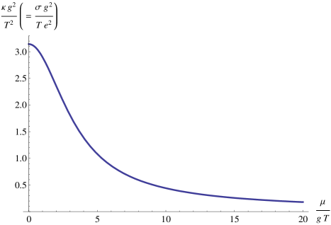
Figure 1: The coefficient of thermal conductivity or The electrical conductivity

We know the asymptotic forms of metric and gauge fields. This information is enough to calculate the first order boundary stress-energy tensor and the current. Using our first order metric and equation (17), we can find the first order stress-energy tensor

$$T_{\mu\nu}=2M(\eta_{\mu\nu}+4u_{\mu}u_{\nu})-2r_{+}^{3}\sigma_{\mu\nu}~{}~{}:=P(\eta_{\mu\nu}+4u_{\mu}u_{\nu})-2\eta\sigma_{\mu\nu}~{}~{},$$ (39)

from which we can read off the viscosity $\eta=r_{+}^{3}$. By restoring $1/(16\pi G)=N_{c}^{2}/8\pi^{2}$, which was set to be 1, we get

$$\eta=\frac{N_{c}^{2}}{8\pi^{2}}r_{+}^{3}=\frac{\pi N_{c}^{2}T^{3}}{8}\left(\frac{1}{2}+\sqrt{\frac{1}{4}+\frac{1}{6}\left(\frac{\mu}{g\pi T}\right)^{2}}\right)^{3}.$$ (40)

where we have used $r_{+}=\frac{\pi T}{2}\left(1+\sqrt{1+\frac{2}{3}(\mu/g\pi T)^{2}}~{}\right)$. In addition, we can also calculate the first order boundary current from (2.2). The current is

$$J^{\mu} = J_{(0)}^{\mu}+J_{(1)}^{\mu}$$ (41)

$$J_{(1)}^{\mu} = \frac{1}{g}\left\{-2\sqrt{3}Q\frac{j_{\beta}\left(r_{+}\right)}{r_{+}^{4}}u^{\lambda}\partial_{\lambda}u^{\mu}+\left(-2\sqrt{3}Q\frac{j_{Q}\left(r_{+}\right)}{r_{+}^{4}}-\frac{\sqrt{3}}{r_{+}}\right)u^{\lambda}F^{(Q)}{}_{\lambda}{}^{\mu}\right.$$ (42)

$$\left.+\left(-2\sqrt{3}Q\frac{j_{F}\left(r_{+}\right)}{r_{+}^{4}}+\frac{e}{g}r_{+}\right)u^{\lambda}F^{\rm ext}{}_{\lambda}{}^{\mu}\right\},$$

where the $j_{\beta}(r_{+})$, $j_{Q}(r_{+})$ and $j_{F}(r_{+})$ are values of each function at the horizon, which can be read from (70) as follows

$$\frac{j_{\beta}\left(r_{+}\right)}{r_{+}^{4}}=\frac{2\left(2r_{+}^{6}+Q^{2}\right)}{8Mr_{+}^{3}}~{}~{},~{}~{}\frac{j_{Q}\left(r_{+}\right)}{r_{+}^{4}}=-\frac{Q}{8Mr_{+}^{3}}~{}~{},~{}~{}\frac{j_{F}\left(r_{+}\right)}{r_{+}^{4}}=-\frac{e}{g}\frac{\sqrt{3}Q}{8Mr_{+}}~{}~{}.$$ (43)

To find physical quantities, we need to change the above equation into familiar form. Using (37) and the temperature of the black hole, we can obtain the final expression of the current which contains dissipative current and contribution from the external field. After some algebra as summarized in the appendix C, the expression turns out to be simplified and given by

$$J_{(1)}^{\mu} = -\frac{\pi^{2}T^{3}r_{+}^{7}}{4g^{2}M^{2}}P^{\mu\nu}\partial_{\nu}\frac{\mu}{T}+\frac{\pi^{2}T^{2}r_{+}^{7}}{4g^{2}M^{2}}u^{\lambda}eF^{\rm ext}{}_{\lambda}{}^{\mu}~{}~{},$$ (44)

$$:= -\kappa P^{\mu\nu}\partial_{\nu}\frac{\mu}{T}+\frac{\sigma}{e}u^{\lambda}F^{\rm ext}{}_{\lambda}{}^{\mu}~{}~{},$$ (45)

where $1/e$ in $\sigma/e$ is inserted to read off the electric conductivity from the electric current $eJ$ rather than the number current $J$. See appendix A.

Now the coefficient of thermal conductivity $\kappa$ and the electrical conductivity are given by

$$\kappa=\frac{\pi^{2}T^{3}r_{+}^{7}}{4g^{2}M^{2}},\;\;\quad\sigma=\frac{\pi^{2}e^{2}T^{2}r_{+}^{7}}{4g^{2}M^{2}}.$$ (46)

To see that the second one is actually the electric conductivity, we notice that $J_{\text{\rm ext}}^{\mu}=\sigma u^{\lambda}F^{\rm ext}_{\lambda}{}^{\mu}$ becomes in non-relativistic limit $J_{\text{\rm ext}}=\sigma(E+v\times B)$ with the $\sigma$ given above. It is easy to show that $\kappa$ can be also written as

$$\kappa={r_{+}\over 4g^{2}}\frac{(2-a)^{2}}{(1+a)^{2}},\;\;\text{with }a=Q^{2}/r_{+}^{6}$$ (47)

so that our result agrees precisely with that of [22], which was obtained from the Kubo formula. Our result of conductivity goes to the known result in [24, 25] for zero charge case . The relation between the thermal and heat conductivity, so called Wiedermann-Franz law:

$$\kappa=\sigma T/e^{2},$$ (48)

is manifest in our case with Lorentz number $1/e^{2}$. Considering the complication of the definition of temperature in the charged black hole and also the difference in the origin of two terms, it is rather surprising to have such similar and simple recombination such that $T\sigma$ and $\kappa$ is proportional to each other. Using $2M=r_{+}^{4}(1+\mu^{2}/(3g^{2}r_{+}^{2}))$ and $r_{+}=\pi T(1+\sqrt{1+2(\mu/g\pi T)^{2}/3})/2$, we can express $\kappa/T^{2}$ and $\sigma/T$ as a function of $\mu/gT$ only:

$$\frac{\kappa}{T^{2}}=\frac{\sigma}{Te^{2}}=\frac{2\pi^{2}}{g^{2}}\frac{1+\sqrt{1+\frac{2}{3}(\frac{\mu}{g\pi T})^{2}}}{\left(1-3\sqrt{1+\frac{2}{3}(\frac{\mu}{g\pi T})^{2}}\right)^{2}}$$ (49)

Fig. 1 shows this as a function of ${\mu}/{gT}$.

We can also calculate the thermal conductivity,

$$\kappa_{T}=\left(\frac{\epsilon+P}{\rho T}\right)^{2}\kappa=4\pi^{2}\cdot\frac{g^{2}}{16\pi G}\cdot\frac{\eta T}{\mu^{2}}.$$ (50)

Notice that $\frac{1}{16\pi G}=\frac{N_{c}^{2}}{8\pi^{2}}$ and $\frac{g^{2}}{16\pi G}$ is 1 and $N_{c}/2N_{f}$ for R-charge and Baryon charge respectively [21].

4 Discussion

We use gauge/gravity duality to determine the structure of the fluid dynamics in the presence of the conserved current and calculated thermal conductivity as well as the electrical conductivity in the presence of the the external electric field. Since the dual of the particle number can regarded as the local charge of the Maxwell field in the bulk, we used the charged black holes in AdS space. For our purpose, the first order in the derivative expansion.

While the determination of the current especially the dissipative part is of highly interesting, going second order or higher order is less interesting from the experimental point of view: what RHIC experiment discovered is that we should neglect the dissipation part almost completely. This perfect liquid behavior is a hall mark of the RHIC experiment. However, LHC experiment may show different behavior due to its much higher collision energy scale. Therefore calculating the transport coefficients may be of some importance for future experiment. It would be also interesting to calculate the similar quantities for other ads space for the application to the solid state physics or M2, M5 brane theories. It would be also interesting to see if this method can help to settle problems of fluid mechanics. [23].

Note added

At the end stage of the this work, we received two papers [26, 27] whose contents are partly overlapping with present paper. Therein, external fields are not included but $T_{\mu\nu}$ and $J_{\mu}$ are calculated up to second order.

Appendix A Number current v.s charge current: Fixing $g$ factors.

For the lagrangian

$$L=-\frac{1}{4g^{2}}F_{\mu\nu}^{2}+J_{\mu}A^{\mu}$$ (51)

the equation of motion is

$$\frac{1}{g^{2}}\partial^{\mu}F_{\mu\nu}=J_{\nu}$$ (52)

If we rewrite the action in terms of the rescaled variable $A_{\mu}/g:=A^{\prime}_{\mu}$,

$$L=-\frac{1}{4}{F^{\prime}}_{\mu\nu}^{2}+gJ_{\mu}A^{\prime\mu},\quad\partial^{\mu}F^{\prime}_{\mu\nu}=gJ_{\nu}:=J^{\prime}_{\nu}.$$ (53)

therefore if $J^{0}=n$ is the number density, $J^{\prime}_{0}=gn$ is the charge density and $J_{\mu}$ is the number current. Also the electromagnetic potential is $A^{\prime}_{\mu}=A_{\mu}/g$.

The number current density $J_{\mu}=2\sqrt{3}Qu_{\mu}/g$ so number density is related to the charge parameter $Q$ by

$$n=2\sqrt{3}Q/g.$$ (54)

The chemical potential for the electric charge density is $\mu^{\prime}=A^{\prime}(\infty)-A^{\prime}(0)=\sqrt{3}Q/r_{+}^{2}$. From the $A.J=A^{\prime}.J^{\prime}$ or $\mu n=\mu^{\prime}J^{\prime}_{0}$ and $J^{\prime}_{0}=gn$, we get $\mu=g\mu^{\prime}$. Then the chemical potential $\mu$ that couples to the number density is $\mu=A_{0}(\infty)-A_{0}(0)$ as was stated in the main text (15). Similar relation hold for electric charge as well as the R-charge.

Appendix B The exact expression for of $j_{i}(r)$ and $a_{i}(r)$

In this appendix we will present exact expressions of $j_{i}(r)$ and $a_{i}(r)$ which can be obtained from coupled differential equations (13) and (14). Integrating (14) from $r=r_{+}$ to $r=\infty$, we get

$$r^{3}f(r)a_{i}^{\prime}(r)-2\sqrt{3}gQ\left(\frac{j_{i}(r)}{r^{4}}-\frac{j_{i}\left(r_{+}\right)}{r_{+}^{4}}\right)=\int_{r_{+}}^{r}dxxS_{i}(x),$$ (55)

where we used the fact that $f(r)$ is zero and $a_{i}(r)$ is not singular at $r=r_{+}$. Using (13) to eliminate $a_{i}^{\prime}(r)$ in (55), we get a second order differential equation of $j_{i}(r)$

$$j_{i}{}^{\prime\prime}(r)-\frac{3}{r}j_{i}^{\prime}(r)-\frac{12Q^{2}}{r^{8}f(r)}j_{i}(r)=\zeta_{i}(r),$$ (56)

where

$$\zeta_{i}(r) \equiv -\frac{12Q^{2}}{r^{4}f(r)}\frac{j_{i}\left(r_{+}\right)}{r_{+}^{4}}+2r^{2}S_{ri}(r)+\frac{2\sqrt{3}Q}{gr^{4}f(r)}\int_{r_{+}}^{r}dxxS_{i}(x)$$ (58)

$$= -3r\partial_{v}\beta_{i}-\frac{2\sqrt{3}Q}{r^{4}f(r)}\left(2\sqrt{3}Q\frac{j_{i}\left(r_{+}\right)}{r_{+}^{4}}-\sqrt{3}\left(\frac{1}{r}-\frac{1}{r_{+}}\right)\left(\partial_{i}Q+Q\partial_{v}\beta_{i}\right)\right.$$

$$\left.+\left(r-r_{+}\right)\frac{e}{g}F_{vi}^{\text{\rm ext}}\right).$$

Two linearly independent homogeneous solutions of this equation are

$$j_{H_{1}}(r) = r^{4}f(r)$$ (59)

$$j_{H_{2}}(r) = j_{H_{1}}(r)\int_{r}^{\infty}\frac{x^{3}dx}{j_{H_{1}}(x){}^{2}}=r^{4}f(r)\int_{r}^{\infty}\frac{dx}{x^{5}f(x)^{2}}.$$ (60)

A particular solution to (56) is found by using method of variation of parameters

$$j_{P}(r)=b_{1}(r)j_{H_{1}}(r)+b_{2}(r)j_{H_{2}}(r),$$ (61)

where

$$b_{1}(r) = -\int_{r}^{\infty}dx\frac{j_{H_{2}}(x)\zeta_{i}(x)}{x^{3}},$$ (62)

$$b_{2}(r) = r^{3}\partial_{v}\beta_{i}+\int_{r}^{\infty}dx\left(\frac{j_{H_{1}}(x)\zeta_{i}(x)}{x^{3}}+3x^{2}\partial_{v}\beta_{i}\right).$$ (63)

Note that $3x^{2}\partial_{v}\beta_{i}$ term cancels the divergence of the integral. Now we can write the general solution to (56)

$$j_{i}(r)=j_{P}(r)+C_{1}j_{H_{1}}(r)+C_{2}j_{H_{2}}(r).$$ (64)

To determine $C_{1}$ and $C_{2}$ we need to find the asymptotic behavior of $j_{i}(r)$

$$j_{i}^{(1)}(r)=C_{1}r^{4}+r^{3}\partial_{v}\beta_{i}+\frac{C_{2}-8MC_{1}}{4}+O\left(\frac{1}{r}\right).$$ (65)

The coefficient $C_{1}$ multiplies a non-normalizable metric deformation, and so is forced to zero by our choice of boundary conditions. The other integration constant $C_{2}$ leads to a nonzero value for $T_{0i}$. We can remove this ambiguity by demanding that $u^{\mu}T^{(n)}_{\mu\nu}=0$, thus $C_{2}$ can be set to zero. In summary,

$$j_{i}(r) = -r^{4}f(r)\int_{r}^{\infty}dxxf(x)\zeta_{i}(x)\int_{x}^{\infty}\frac{dy}{y^{5}f(y)^{2}}$$ (66)

$$+r^{4}f(r)\left(\int_{r}^{\infty}\frac{dx}{x^{5}f(x)^{2}}\right)\left(r^{3}\partial_{v}\beta_{i}+\int_{r}^{\infty}dx\left[xf(x)\zeta_{i}(x)+3x^{2}\partial_{v}\beta_{i}\right]\right).$$

Having the expression of $j_{i}(r)$, $a_{i}(r)$ is obtained by integrating (13)

$$a_{i}(r)=-g\int_{r}^{\infty}dr\frac{x^{3}}{\sqrt{3}Q}\left[\frac{x}{2}\left(\frac{j_{i}^{\prime}(x)}{x^{3}}\right)^{\prime}-S_{ri}(x)\right],$$ (67)

where we chose the gauge to make $a_{i}(r)$ vanishes at infinity.

Since we are interested in boundary physics, we present asymptotic behaviors of these functions here:

$$j_{i}(r) \approx r^{3}\partial_{v}\beta_{i}-\frac{2\sqrt{3}Q}{5r}\frac{e}{g}F_{vi}^{\text{\rm ext}}+\frac{1}{r^{2}}\left(-Q^{2}\frac{j_{i}\left(r_{+}\right)}{r_{+}^{4}}-\frac{Q}{2r_{+}}\left(\partial_{i}Q+Q\partial_{v}\beta_{i}\right)\right.$$ (68)

$$\left.+\frac{r_{+}Q}{2\sqrt{3}}\frac{e}{g}F_{vi}^{\text{\rm ext}}\right),$$

$$a_{i}(r) \approx \frac{1}{r}eF_{vi}^{\text{\rm ext}}+\frac{1}{r^{2}}\left(\sqrt{3}gQ\frac{j_{i}\left(r_{+}\right)}{r_{+}^{4}}+\frac{\sqrt{3}g}{2r_{+}}\left(\partial_{i}Q+Q\partial_{v}\beta_{i}\right)-\frac{r_{+}}{2}eF_{vi}^{\text{\rm ext}}\right).$$ (69)

Still we have undetermined constant, $j_{i}(r_{+})$. Taking $r\to r_{+}$ limit to (66) yields an equation of $j_{i}(r_{+})$. After some calculations we get

$$\frac{j_{i}\left(r_{+}\right)}{r_{+}^{4}} = \frac{2r_{+}^{2}\left(2r_{+}^{4}+r_{+}^{2}r_{-}^{2}+r_{-}^{4}\right)\partial_{v}\beta_{i}-Q\left(\partial_{i}Q+Q\partial_{v}\beta_{i}\right)-\sqrt{3}r_{+}^{2}Q\frac{e}{g}F_{vi}^{\text{\rm ext}}}{6r_{+}Q^{2}-2r_{+}^{3}\left(-2r_{+}^{4}+r_{+}^{2}r_{-}^{2}+r_{-}^{4}\right)}$$ (70)

$$= \frac{2\left(2r_{+}^{6}+Q^{2}\right)\partial_{v}\beta_{i}-Q\left(\partial_{i}Q+Q\partial_{v}\beta_{i}\right)-\sqrt{3}r_{+}^{2}Q\frac{e}{g}F_{vi}^{\text{\rm ext}}}{8Mr_{+}^{3}}.$$

From the definition

$$j_{i}(r) = j_{\beta}(r)\partial_{v}\beta_{i}+j_{Q}(r)(\partial_{i}Q+Q\partial_{v}\beta_{i})+j_{F}(r)F^{\rm ext}_{vi},$$ (71)

we can read off the result (43).

Appendix C Current expression and useful relations

To obtain the current expression of (44), we massage (42) and get following form

$$J_{(1)}^{\mu}=\frac{1}{g}\left[-\frac{\sqrt{3}Q}{4M}\left(2r_{+}^{3}+\frac{Q^{2}}{r_{+}^{3}}\right)(3u^{\lambda}\partial_{\lambda}u^{\mu}+P^{\mu\lambda}\partial_{\lambda}\log Q)+\left(\frac{3Q^{2}}{4Mr_{+}}+r_{+}\right)u^{\lambda}F_{\lambda\mu}^{\text{ext}}\right]~{}~{}.$$ (72)

We need to change first term into derivatives of physical quantities. For this, we use more useful form of (37),

$$u^{\lambda}\partial_{\lambda}u^{\mu}=\frac{\sqrt{3}Q}{4M}\frac{e}{g}u^{\lambda}F_{\lambda\mu}^{\text{ext}}-\frac{1}{4M}P^{\mu\nu}\partial_{\nu}M~{}.$$ (73)

Using this equation and other relations between physical quantities, one can get our result (44). We write down the useful relations for this algebra as

$$Q=\frac{\mu r_{+}^{2}}{\sqrt{3}g},$$ (74)

$$r_{+}^{2}r_{-}^{2}+r_{-}^{4}=\frac{\mu^{2}r_{+}^{2}}{3g^{2}}=2M-r_{+}^{4},$$ (75)

$$T=\frac{1}{2\pi r_{+}^{3}}\left(2r_{+}^{4}-r_{+}^{2}r_{-}^{2}-r_{-}^{4}\right)=\frac{6r_{+}^{2}-\mu^{2}/g^{2}}{6\pi r_{+}}=\frac{3r_{+}^{4}-2M}{2\pi r_{+}^{3}}~{}.$$ (76)

References

• [1] J.M. Maldacena, Adv. Theor. Math. Phys. 2 (1998) 231, [arXiv:hep-th/9711200].
• [2] S.S. Gubser, I.R. Klebanov and A.M. Polyakov, Phys. Lett. B428 (1998) 105, [arXiv:hep-th/9802109].
• [3] E. Witten, Adv. Theor. Math. Phys. 2 (1998) 253, [arXiv:hep-th/9802150].
• [4] G. Policastro, D.T. Son and A.O. Starinets, Phys. Rev. Lett.  87 (2001) 081601, [arXiv:hep-th/0104066].
• [5] P. Kovtun, D.T. Son and A.O. Starinets, JHEP 0310 (2003) 064,
[arXiv:hep-th/0309213].
• [6] A. Buchel and J.T. Liu, Phys. Rev. Lett.  93 (2004) 090602,
[arXiv:hep-th/0311175].
• [7] E. Shuryak, S.-J. Sin and I. Zahed, J. Korean Phys. Soc.  50 (2007) 384,
[arXiv:hep-th/0511199].
• [8] K.-Y. Kim, S.-J. Sin and I. Zahed, [arXiv:hep-th/0608046].
• [9] N. Horigome and Y. Tanii, JHEP 0701 (2007) 072, [arXiv:hep-th/0608198].
• [10] S. Nakamura, Y. Seo, S.-J. Sin and K.P. Yogendran, [arXiv:hep-th/0611021].
• [11] S. Kobayashi, D. Mateos, S. Matsuura, R.C. Myers and R.M. Thomson, JHEP 0702 (2007) 016, [arXiv:hep-th/0611099].
• [12] S. Nakamura, Y. Seo, S.-J. Sin and K.P. Yogendran, [arXiv:0708.2818[hep-th]].
• [13] Nonlinear Fluid Dynamics from Gravity. Sayantani Bhattacharyya , Veronika E Hubeny , Shiraz Minwalla , Mukund Rangamani. JHEP 0802:045,2008. arXiv:0712.2456 [hep-th]
• [14] L.D. Landau and E.M. Lifshitz, Fluid mechanics, Pergamon Press, New York, 1987, 2nd ed.
• [15] D. T. Son and A. O. Starinets, JHEP 0603, 052 (2006) [arXiv:hep-th/0601157].
• [16] A Stress tensor for Anti-de Sitter gravity. Vijay Balasubramanian , Per Kraus . Commun.Math.Phys.208:413-428,1999. hep-th/9902121
• [17] Black Hole Dynamics From Atmospheric Science. Mark Van Raamsdonk . JHEP 0805:106,2008. arXiv:0802.3224[hep-th]
• [18] Sayantani Bhattacharyya, R. Loganayagam, Shiraz Minwalla, Suresh Nampuri, Sandip P. Trivedi, Spenta R. Wadia, “Forced Fluid Dynamics from Gravity”, arXiv:0806.0006[hep-th].
• [19] M. Haack and A. Yarom, “Nonlinear viscous hydrodynamics in various dimensions using AdS/CFT,” arXiv:0806.4602 [hep-th].
• [20] S. Bhattacharyya, R. Loganayagam, I. Mandal, S. Minwalla and A. Sharma, “Conformal Nonlinear Fluid Dynamics from Gravity in Arbitrary Dimensions,” arXiv:0809.4272 [hep-th].
• [21] S.-J. Sin, JHEP 0710 (2007) 078, [arXiv:0707.2719[hep-th]].
• [22] X. H. Ge, Y. Matsuo, F. W. Shu, S. J. Sin and T. Tsukioka, “Density Dependence of Transport Coefficients from Holographic Hydrodynamics”, arXiv:0806.4460 [hep-th].
• [23] K. Tsumura and T. Kunihiro, “Stable First-order Particle-frame Relativistic Hydrodynamics for arXiv:0709.3645 [nucl-th].
• [24] S. Caron-Huot, P. Kovtun, G. D. Moore, A. Starinets and L. G. Yaffe, JHEP 0612, 015 (2006) [arXiv:hep-th/0607237].
• [25] A. Karch and A. O’Bannon, JHEP 0709, 024 (2007) [arXiv:0705.3870 [hep-th]].
• [26] N. Banerjee, J. Bhattacharya, S. Bhattacharyya, S. Dutta, R. Loganayagam and P. Surowka, “Hydrodynamics from charged black branes,” arXiv:0809.2596 [hep-th].
• [27] J. Erdmenger, M. Haack, M. Kaminski and A. Yarom, “Fluid dynamics of R-charged black holes,” arXiv:0809.2488 [hep-th].