Speckle instability: coherent effects in nonlinear disordered media

Abstract

We numerically investigate the properties of speckle patterns formed by nonlinear point scatterers. We show that, in the weak localization regime, dynamical instability appears, eventually leading to chaotic behavior of the system. Analysing the statistical properties of the instability thresholds for different values of the system size and disorder strength, a scaling law is emphasized. The later is also found to govern the smallest decay rate of the linear system, putting thus forward the crucial importance of interference effects. This is also underlined by the fact that coherent backscattering is still observed even in the chaotic regime.

As first described by Anderson in 1958, the impact of disorder on the transport properties of waves, depending on the dimensionality and the disorder strength, ranges from weak to strong localization. In the case of matter waves, the localization of Bose-Einstein condensates (BEC) is, at present, a very active research topic investigated by several experimental and theoretical groups clement05 ; fort05 ; schulte05 ; paul07 ; robert07 ; lsp07 ; skipetrov08 ; hartung08 , in particular with the recent observation of the (1D) localization of matter waves in a disordered optical potentials lsp08 ; roati08 . Although, in these experiments, the atom-atom interactions were negligible, the basic question remains how effects of interference between multiply scattered waves, such as weak or strong localization, are affected by interactions.

BEC’s in disordered potentials appear to be good candidates to study these questions, since, in the mean field regime, the condensate is still described by a single coherent wave function governed by a nonlinear wave equation (Gross-Pitaevski equation). Thus, the condensate in principle retains its ability to display interference effects also in presence of (not too strong) interactions. Similar nonlinear equations describe propagation of light in disordered nonlinear media skipetrov . In contrast, the situation is quite different in the case of electronic transport altshuler99 , where the interactions combined with finite temperature effects give rise to dephasing, which in general destroy the disorder-induced coherent effects.

Even if the theoretical description of coherent effects in nonlinear disordered systems is far from complete, an important step was done recently by the development of a diagrammatic theory for coherent backscattering in presence of nonlinearity wellens08 . This approach relies on the assumption of a unique stationary solution of the nonlinear wave equation under consideration. This assumption is expected to be valid for very weak nonlinearities (which, however, may still considerably affect the height of the coherent backscattering cone wellens08 ; hartung08 ). On the other hand, it is known that larger nonlinearities can induce speckle instabilities, such that no stationary state is reached at long times hartung08 ; paul05 . A clear explanation for the physical origin of this effect, however, is still missing. Theoretical predictions of the nonlinearity threshold above which instabilities develop, were attempted in spivak ; skipetrov , but, to our knowledge, these results have not yet been confirmed by experiments or numerical simulations. For this reason, we investigate, in this letter, the dynamical properties of the speckle patterns generated by nonlinear point scatterers.

More precisely, we consider an assembly of $N$ point-like scatterers located at randomly chosen positions $\mathbf{r}_{i}$, $i=1,\dots,N$, inside a sphere of volume $V$ illuminated by a plane wave $\mathbf{k}_{L}$. The field amplitude $E_{i}$ at scatterer $i$ results as the sum of the incident wave and the field radiated by all other scatterers:

$$E_{i}=e^{i\mathbf{k}_{L}\cdot\mathbf{r}_{i}}+\sum_{j\neq i}\frac{e^{ik|{\bf r}_{i}-{\bf r}_{j}|}}{k|{\bf r}_{i}-{\bf r}_{j}|}d_{j},$$ (1)

where $k=|{\bf k}_{L}|=2\pi/\lambda$, and the field amplitudes are measured in units of the incident plane wave amplitude. $d_{j}$ describes the dipole induced inside scatterer $j$. For simplicity, we will consider only scalar fields in this letter.

As for the induced dipole, we consider a nonlinear response $d=g\left(|E|^{2}\right)E$, with

$$g(I)=i\frac{e^{i\alpha I}+1}{2}.$$ (2)

For $\alpha=0$, this model corresponds to a resonant point scatterer. The nonlinearity $\alpha$ induces a phase shift proportional to the local intensity $I$, which amounts to a shift of the scatterer’s resonance frequency. For small $\alpha$, Eq. (2) reduces to a $\chi^{(3)}$-nonlinearity; furthermore, for real values of $\alpha$, the optical theorem is fulfilled, ensuring energy conservation. The above set of $N$ complex equations (1), with the replacement (2), is formally written as $\mathbf{F}(\mathbf{E},\alpha)=\mathbf{0}$, where $\mathbf{F}$ and $\mathbf{E}$ are real vectors of dimension $2N$.

Starting from the linear solution ($\alpha=0$) for a given configuration of the scatterers, a numerical scheme, based on a Newton-Krylov method, allows to continuously follow the solution $\mathbf{E}(\alpha)$, which fulfills

$$\frac{d\mathbf{E}}{d\alpha}=-{\mathbf{M}}^{-1}\frac{\partial\mathbf{F}}{\partial\alpha}$$ (3)

with the Jacobian matrix $\mathbf{M}=\frac{\partial\mathbf{F}}{\partial\mathbf{E}}$. If $\mathbf{M}$ has a vanishing eigenvalue, this gives rise to a turning point in the curve $\mathbf{E}(\alpha)$, such that several solutions of Eq. (1) coexist for the same value of $\alpha$.

As an example, we plot in Fig. 1 (top) the intensity $I_{\mathrm{out}}$, scattered into the direction opposite to the incident wave as a function of $\alpha$, for a specific configuration of $N=1000$ scatterers randomly distributed in a sphere with density $n=N/V$ such that $n\lambda^{3}=1$. For $\alpha=0$, these parameters correspond to mean free path $\ell=20/k$ and optical thickness (measured along the diameter $2R$ of the sphere) $2R/\ell_{0}=4$. In Fig. 1 (top), we clearly notice the existence of several stationary solutions for $\alpha>0.3$, and in particular for $\alpha>0.6$ (see inset). Fig. 1(middle) shows the smallest module $|\lambda|_{\mathrm{min}}$ of all eigenvalues of the matrix $\mathbf{M}$. At every turning point, the curve $|\lambda|_{\mathrm{min}}(\alpha)$ touches the horizontal axis, as expected.

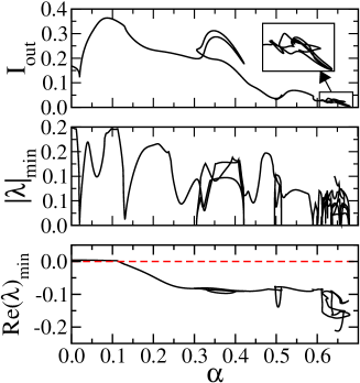
Figure 1: (Color online) For a given random configuration of $N=1000$ scatterers with density $n\lambda^{3}=1$, the top plot depicts the backward intensity $I_{\mathrm{out}}$ as a function of the nonlinearity strength $\alpha$. For $\alpha>0.3$, several stationary solutions coexist. The middle plot shows the smallest module of all eigenvalues of the stability matrix $\mathbf{M}$. At each turning point, $\mathbf{M}$ exhibits a vanishing eigenvalue. The bottom plot depicts the smallest real part of all eigenvalues of $\mathbf{M}$. The dashed line indicates the stability threshold defined by $\mathrm{Re}(\lambda)=0$. At $\alpha\simeq 0.1$, the solution becomes unstable, and the instability then increases with $\alpha$.

However, even if multiple stationary solutions coexist, one will observe speckle instability, i.e. a time dependent solution persisting at long time, only if these solutions are dynamically unstable. To investigate the dynamical behaviour, we use the following relaxation model for the time evolution of the dipole $d(t)$:

$$\dot{d}(t)=-\frac{\Gamma}{2}\biggl{(}d(t)-g(I)E)\biggr{)},$$ (4)

where $\Gamma/2$ corresponds to the inverse relaxation time. $E$ and $I$ are now the instantaneous local field and intensity. We assume $\Gamma\ll c/R$, such that the field propagation can be considered as instantaneous within the radius $R$ of the cloud. According to this model, small deviations $\delta\mathbf{E}(t)=\mathbf{E}(t)-\mathbf{E}^{\mathrm{st}}$ from the stationary solution $\mathbf{E}^{\mathrm{st}}$ fulfill the following set of equations:

$$\dot{\delta\mathbf{E}}(t)=-\frac{\Gamma}{2}\mathbf{M}\delta\mathbf{E},$$ (5)

Hence, the stationary solution is stable if all eigenvalues of the matrix $M$ have a positive real part. In Fig. 1 (bottom), we plot the smallest real part of all eigenvalues along the stationary solution shown on the top. Just above $\alpha=0.1$, the solution becomes unstable and the instability increases with $\alpha$. Furthermore, in the region of multiple solutions (see around $\alpha=0.5$, for instance), the different solutions have different instability rates. As a closer inspection reveals, the branch between the two turning points is the most unstable one, exactly like in the standard bistability scheme boyd . However, whereas in the usual scheme the two other branches would correspond to stable solutions, leading to a bistable behavior, they are, in the present case, also unstable.

In summary, Fig. 1(bottom) reveals that, for the specific configuration of scatterers under consideration, no stable stationary solution exists for $\alpha>0.1$. Hence, we expect that, in this regime, the actual dynamics of the system does not converge towards a stationary state, but remains time-dependent even in the long-time limit. This is confirmed by Fig. 2, where we plot, for the same configuration of scatterers as in Fig. 1, the backscattered intensity as a function of time for different values of the nonlinearity strength $\alpha$. One clearly observes a transition from the stable stationary solution at $\alpha=0$ to a chaotic-like behavior at $\alpha=1$. For intermediate values, stable periodic solutions are obtained, indicating that, for those values, the stationary solutions are already unstable. Let us stress that the bifurcation from the stable to the unstable regime does not necessarily occur at values of the nonlinearity for which many stationary solutions coexist. Indeed, since our dynamical system has a very large number of degrees of freedom ($2N$) and, in addition, is not a Hamiltonian one, many possible bifurcation scenarios are in principle possible, including for example strange attractors rasband . A more detailed analysis would require the complete determination of the underlying dynamical structure (periodic orbits, limit cycles…), which is beyond the scope of this Letter.

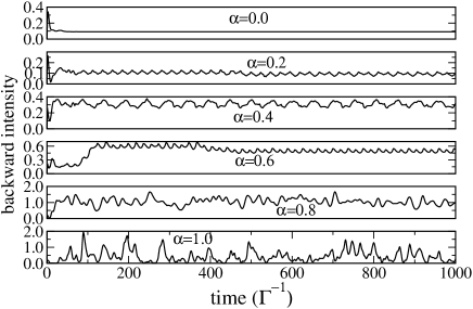
Figure 2: Typical evolution of the intensity in the backward direction as a function of time for the same configuration of scatterers as in Fig. 1, and for different values of the nonlinearity strength $\alpha$. One clearly observes a transition from a stable stationary solution for $\alpha=0$ to a chaotic-like behavior for $\alpha=1$. For intermediate values, stable periodic solutions are obtained, emphasizing that, for those values, the stationary solutions are already unstable.

The preceding discussion refers to a given single configuration of scatterers. Although it has been chosen as a representative example of the transition to the unstable regime, more information can be obtained when performing a statistical analysis of the system properties over an ensemble of different configurations. Fig. 3 (top) displays the cumulative distributions of instability thresholds, denoted $P_{\mathrm{inst}}(\alpha)$, for different system parameters. Hence, we have plotted, for different numbers $N$ and optical densities $n\lambda^{3}$ of scatterers, the proportion of unstable configurations as a function of the nonlinearity strength $\alpha$. As expected, if we fix the number of scatterers, the instability occurs earlier (i.e. the distributions are shifted towards smaller $\alpha$) for increasing density (i.e. disorder strength). On the other hand, if we fix the density, instable configurations are more frequently encountered with increasing number of scatterers (i.e. system size). However, both variations are not independent: as the figure clearly reveals, the statistical distribution depends only on a single parameter, namely $p=N\times n\lambda^{3}$. In particular, the average threshold, $\left\langle\alpha_{\mathrm{inst}}\right\rangle$, depends linearly on $p^{-1}$, see Fig. 3 (bottom, left).

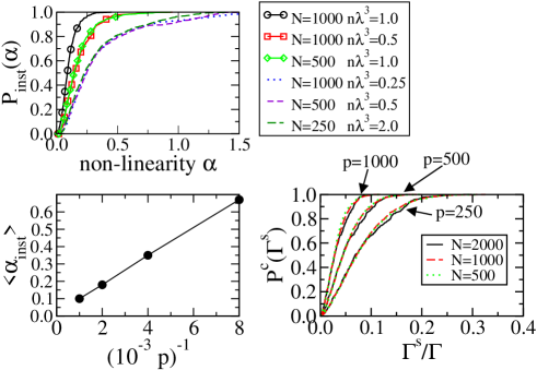
Figure 3: (Color online) On the top, the cumulative distributions of instability thresholds are plotted for different numbers $N$ and densities $n\lambda^{3}$ of scatterers. A scaling law is revealed, according to which the distributions depend only on a single parameter $p=N\times n\lambda^{3}$. The bottom left plot shows the average threshold to depend linearly on $p^{-1}$. The bottom right plot displays the distribution $P^{c}(\Gamma^{s})$ of the smallest linear decay rate $\Gamma_{s}$, which exhibits the same scaling law in terms of the parameter $p$. This strongly emphasizes the crucial role played by the interference effects for the speckle instability.

As we have checked, for large $p$, the resulting instability thresholds are small enough so that first order perturbation theory with respect to the nonlinearity strength $\alpha$ can be applied. Hence, we expect the statistics of instability thresholds to be closely related to properties of the linear system, in particular the real parts of the eigenvalues of $\mathbf{M}(\alpha=0)$. The latter define the decay rates $\Gamma^{s}$ of the linear system rusek00 ; pinheiro04 . Since the occurence of a single negative eigenvalue is already sufficient for the instability to occur, the state with the smallest decay rate (or, equivalently, longest lifetime) attains a particular importance. Therefore, we have plotted in Fig. 3(bottom, right) the cumulative distribution of the smallest rate $\Gamma^{s}$ for different numbers $N$ of scatterers and densities $n\lambda^{3}$. Here, the solid lines correspond to $N=2000$ and (from left to right) $n\lambda^{3}=$0.5, 0.25 and 0.125, the long-dashed lines to $N=1000$ and (from left to right) $n\lambda^{3}=$1, 0.5 and 0.25 and the dotted lines to $N=500$ and (from left to right) $n\lambda^{3}=$2, 1. and 0.5. And indeed, we find the distributions to be governed by the same parameter $p=N\times n\lambda^{3}$ which also determines the statistics of instability thresholds. From these data, the average value $\Gamma/\left<\Gamma^{s}\right>$, i.e. the longest lifetime, is found, as a crude estimate, to scale like $p^{2/3}$. This time is much longer than the Thouless time, i.e the longest time predicted within diffusion approximation, which, in $\Gamma^{-1}$ unit, scales like $(pn\lambda^{3})^{2/3}$ (i.e. the square of the optical thickness). This difference strongly emphasizes that interference effects, which enhance the lifetime of a particular single mode with respect to the diffusive Thouless time, are deeply involved in the speckle instability. Due to its long lifetime, such a ”prelocalized” mode apalkov02 almost behaves like a perfect cavity, and is therefore much more severely affected by the nonlinearity than short-lived modes and, thus, eventually allows instability to settle. We note that a similar argument was also put forward to explain the appearance of discrete peaks in the emission spectrum of the coherent random laser cao . Let us note that the instability threshold of our nonlinear point scatterers system differ from the one predicted in the case of linear scatterers in a $\chi^{(3)}$ nonlinear medium skipetrov , for which no instability should occur if the nonlinearity is small enough for first order perturbation theory to apply. Further research is necessary in order to characterize the relevant properties of nonlinear disordered systems, leading to different scenarios for the development of speckle instabilities.

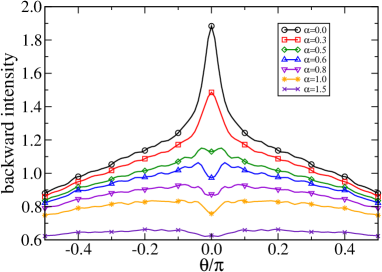
Figure 4: (Color online) Configuration average of the intensity $\left\langle I(\theta,t)\right\rangle$, scattered at time $t=1000\Gamma^{-1}$, in the direction $\theta$, where $\theta=0$ corresponds to exact backscattering, for 1000 different configurations of $N=1000$ scatterers with density $n\lambda^{3}=1$. Although the coherent backscattering cone at first decreases with increasing nonlinearity, the occurence of a dip at larger nonlinearities proves that coherent effects survive in the time dependent regime $\alpha\gtrsim 0.3$, and even in the fully chaotic one $\alpha\gtrsim 1$.

Finally, we address the question of coherent transport in the unstable regime. For this purpose, we compute the coherent backscattering (CBS) cone $\left\langle I(\theta,t)\right\rangle$, i.e. the configuration average of the intensity scattered at a time $t$ in the direction $\theta$, where $\theta=0$ corresponds to the exact backward direction. Numerically, we observe that after, typically, few $100\Gamma^{-1}$, the average intensity $\left\langle I(\theta,t)\right\rangle$ becomes time-independent. We plot this stationary value as a function of $\theta$ in Fig. 4, where the average is performed over 1000 random configurations with the same parameters ($N=1000$ and $n\lambda^{3}=1$) as for the configuration examined in Figs. 1 and 2. Obviously, the net effect of the nonlinearity is the reduction of the CBS cone height, and the formation of a dip at larger nonlinearities hartung08 . According to the theory presented in wellens08 , this effect can be qualitatively explained by a dephasing between reversed scattering induced by the nonlinearity. In the present context, however, the most important point is that a coherent effect still survives in the time dependent regime at $\alpha\gtrsim 0.3$, and even in the fully chaotic one at $\alpha\gtrsim 1$. A possible explanation can be put forward when considering the time evolution depicted in Fig 2: the typical timescale is much larger than the scatterer response time $\Gamma^{-1}$, such that the intensity pattern is almost fixed for a photon scattered along short paths inside the medium.

In summary, using a model of nonlinear point scatterers, we have analysed the dynamical instability properties of the speckle patterns, and observed the transition from a regime with a unique, stable and stationary solution towards chaotic-like behavior. In addition, we have shown that the statistical properties of the instability thresholds are determined by the same parameter as the smallest decay rates of the linear system, putting thus forward the crucial role played by interference effects for the speckle instabilities. Furthermore, we have shown that, quite surprisingly, the coherent backscattering effects are not erased in the time dependent regime, even not in the chaotic one. Obviously, it would be very interesting to perform similar studies in the strongly localized regime ($k\ell\lesssim 1$). Although our argument based on the decay rates of the linear system would then suggest the appearance of instabilities for any small amount of nonlinearity, our results also leave open the possibility to observe strong localization even in presence of nonlinearity, depending on the timescale on which the instabilities develop. The authors would like to thank S. Skipetrov, C. Miniatura and D. Delande for fruitful discussions.

References

- (1) D. Clément et al., Phys. Rev. Lett 95 170409 (2005)
- (2) C. Fort et al., Phys. Rev. Lett. 95 170410 (2005)
- (3) T. Schulte et al., Phys. Rev. Lett. 95 170411 (2005)
- (4) L. Sanchez-Palencia et al., Phys. Rev. Lett. 98, 210401 (2007).
- (5) T. Paul, P. Schlagheck, P. Leboeuf, and N. Pavloff, Phys. Rev. Lett. 98, 210602 (2007).
- (6) R. Kuhn, O. Sigwarth, C. Miniatura, D. Delande and C.A. Müller, New J. Phys. 9, 161 (2007).
- (7) S.E. Skipetrov, A. Minguzzi, B.A. van Tiggelen, and B. Shapiro, Phys. Rev. Lett. 100, 165301 (2008).
- (8) M. Hartung, T. Wellens, C.A. Müller, K. Richter, and P. Schlagheck, Phys. Rev. Lett. 101, 020603 (2008).
- (9) J. Billy et al., Nature 453, 891 (2008).
- (10) G. Roati et. al., Nature 453, 895 (2008).
- (11) S. Skipetrov and R. Maynard, Phys. Rev. Lett. 85, 736 (2000).
- (12) I.L. Aleiner, B.L. Altshuler, and M.E. Gershenson, Waves Random Media 9, 201 (1999).
- (13) T. Wellens and B. Grémaud, Phys. Rev. Lett. 100, 033902 (2008).
- (14) T. Paul et al., Phys. Rev. A 72, 063621 (2005).
- (15) B. Spivak and A. Zyuzin, Phys. Rev. Lett. 84, 1970 (2000).
- (16) R. W. Boyd, Nonlinear Optics Academic Press, San Diego, (1992).
- (17) S.N. Rasband, Chaotic dynamics of nonlinear systems, Ed. Wiley (1990).
- (18) M. Rusek, J. Mostowski, and A. Orłowski, Phys. Rev.‘A 61, 022704 (2000)
- (19) F. A. Pinheiro, M. Rusek, A. Orłowski, and B.A. van Tiggelen, Phys. Rev. E 69, 026605 (2004)
- (20) V.M. Apalkov, M.E. Raikh, and B. Shapiro, Phys. Rev. Lett. 89, 016802 (2002).
- (21) H. Cao, Waves Random Media 13, R1 (2003).