Fundamental Theorem of Calculus

Abstract

A simple but rigorous proof of the Fundamental Theorem of Calculus is given in geometric calculus, after the basis for this theory in geometric algebra has been explained. Various classical examples of this theorem, such as the Green’s and Stokes’ theorem are discussed, as well as the new theory of monogenic functions, which generalizes the concept of an analytic function of a complex variable to higher dimensions.

Keywords: geometric algebra, geometric calculus, Green’s theorem, monogenic functions, Stokes’ theorem.

AMS 2000 Subject Classification : 32A26, 58A05, 58A10, 58A15.

Introduction

Every student of calculus knows that integration is the inverse operation to differentiation. Things get more complicated in going to the higher dimensional analogs, such as Green’s theorem in the plane, Stoke’s theorem, and Gauss’ theorem in vector analysis. But the end of the matter is nowhere in sight when we consider differential forms, tensor calculus, and differential geometry, where important analogous theorems exist in much more general settings. The purpose of this article is to express the fundamental theorem of calculus in geometric algebra, showing that the multitude of different forms of this theorem fall out of a single theorem, and to give a simple and rigorous proof. An intuitive proof of the fundamental theorem in geometric algebra was first given in [1]. The basis of this theorem was further explored in [2], [3]. We believe that the geometric algebra version of this important theorem represents a significant improvement and generalization over other forms found in the literature, such as for example in [4].

Geometric algebra was introduced by William Kingdon Clifford in 1878 as a generalization and unification of the ideas of Hermann Grassmann and William Hamilton, who came before him [5], [6]. Whereas Hamilton’s quaternions are well known and Grassmann algebras are known in various guises such as the exterior algebras of differential forms [7], and anti-symmetric tensors, the full generality and utility of Clifford’s geometric algebras are just beginning to be appreciated [8], [9]. We hope that this paper will attract the attention of the scientific community to the generality and beauty of this formalism. What follows is a short introduction to the basic ideas of geometric algebra that are used in this paper.

Geometric algebra

Let $\{{\bf e}_{i}\}_{i=1}^{n}$ be the standard orthonormal basis of the $n$-diminsional euclidean space $I\!\!R^{n}$. Vectors ${\bf a},{\bf b}\in I\!\!R^{n}$ can be represented in the alternative forms

$${\bf a}=(a^{1}\ a^{2}\ \cdots\ a^{n})=\sum_{i}a^{i}{\bf e}_{i}\ \ {\rm and}\ \ {\bf b}=(b^{1}\ b^{2}\ \cdots\ b^{n})=\sum_{i}b^{i}{\bf e}_{i},$$

and their inner product is given by

$${\bf a}\cdot{\bf b}=|{\bf a}||{\bf b}|\cos\theta=\sum_{i}a^{i}b^{i}$$

where $\theta$ is the angle between them.

The history of mathematics begins with the invention of the natural numbers [10], and continues with successive extensions of the number concept [11]. The associative geometric algebra ${\cal G}_{n}={\cal G}_{n}(I\!\!R^{n})$ of the euclidean space $I\!\!R^{n}$ can be thought of as the geometric extension of the real number system $I\!\!R$ to include $n$ new anticommuting square roots of unity, which we identify with the basis vectors ${\bf e}_{i}$ of $I\!\!R^{n}$, and their geometric products. This is equivalent to saying that each vector ${\bf a}\in I\!\!R^{n}$ has the property that

$${\bf a}^{2}={\bf a}{\bf a}={\bf a}\cdot{\bf a}=|{\bf a}|^{2},$$

where $|{\bf a}|$ is the euclidean length or magnitude of the vector ${\bf a}$.

The fundamental geometric product ${\bf a}{\bf b}$ of the vectors ${\bf a},{\bf b}\in I\!\!R^{n}\subset{\cal G}_{n}$ can be decomposed into the symmetric inner product, and the anti-symmetic outer product

$${\bf a}{\bf b}=\frac{1}{2}({\bf a}{\bf b}+{\bf b}{\bf a})+\frac{1}{2}({\bf a}{\bf b}-{\bf b}{\bf a})={\bf a}\cdot{\bf b}+{\bf a}\wedge{\bf b}=|{\bf a}||{\bf b}|e^{i\theta},$$ (1)

where ${\bf a}\cdot{\bf b}=\frac{1}{2}({\bf a}{\bf b}+{\bf b}{\bf a})$ is the inner product and

$${\bf a}\wedge{\bf b}=\frac{1}{2}({\bf a}{\bf b}-{\bf b}{\bf a})=|{\bf a}||{\bf b}|i\sin\theta$$

is the outer product of the vectors ${\bf a}$ and ${\bf b}$. The outer product ${\bf a}\wedge{\bf b}$ is given the geometric interpretation of a directed plane segment or bivector and characterizes the direction of the plane of the subspace of $I\!\!R^{n}$ spanned by the vectors ${\bf a}$ and ${\bf b}$. The unit bivector $i$ orients the plane of the vectors ${\bf a}$ and ${\bf b}$, and has the property that $i^{2}=-1$. See Figure 1. The last equality in (1) expresses the beautiful Euler formula for the geometric product of the two vectors ${\bf a}$ and ${\bf b}$.

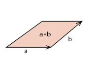
Figure 1: The bivector ${\bf a}\wedge{\bf b}$ is obtained by sweeping the vector ${\bf b}$ out along the vector ${\bf a}$. Also shown is the unit bivector $i$ in the plane of ${\bf a}$ and ${\bf b}$.

The real $2^{n}$-dimensional geometric algebra ${\cal G}_{n}={\cal G}_{n}(I\!\!R^{n})$ has the standard basis

$${\cal G}_{n}={\rm span}\{1,{\bf e}_{\lambda_{1}},{\bf e}_{\lambda_{2}},\dots,{\bf e}_{\lambda_{n}}\},$$

where the $\pmatrix{n\cr k}$ $k$-vector basis elements of the form ${\bf e}_{\lambda_{k}}$ are defined by

$${\bf e}_{\lambda_{k}}={\bf e}_{i_{1}\ldots i_{k}}={\bf e}_{i_{1}}\cdots{\bf e}_{i_{k}}$$

for each $\lambda_{k}=i_{1}\cdots i_{k}$ where $1\leq i_{1}<\cdots<i_{k}\leq n$. Thus, for example, the $2^{3}$-dimensional geometric algebra of $I\!\!R^{3}$ has the standard basis

$${\cal G}_{3}={\rm span}\{1,{\bf e}_{1},{\bf e}_{2},{\bf e}_{3},{\bf e}_{12},{\bf e}_{13},{\bf e}_{23},{\bf e}_{123}\}.$$

We denote the pseudoscalar of $I\!\!R^{n}$ by the special symbol $I={\bf e}_{1\ldots n}$. The pseudoscalar gives a unique orientation to $I\!\!R^{n}$ and $I^{-1}={\bf e}_{n\ldots 1}$.

Let ${\bf a}$ be a vector, and ${\bf B}_{k}$ be a $k$-vector in ${\cal G}_{n}$ where $k\geq 1$. Just as for (1), we decompose the product ${\bf a}{\bf B}_{k}$ into symmetric and anti-symmetric parts,

$${\bf a}{\bf B}_{k}=\frac{1}{2}({\bf a}{\bf B}_{k}+(-1)^{k+1}{\bf B}_{k}{\bf a})+\frac{1}{2}({\bf a}{\bf B}_{k}-(-1)^{k+1}{\bf B}_{k}{\bf a})={\bf a}\cdot{\bf B}_{k}+{\bf a}\wedge{\bf B}_{k},$$ (2)

where

$${\bf a}\cdot{\bf B}_{k}=\frac{1}{2}({\bf a}{\bf B}_{k}+(-1)^{k+1}{\bf B}_{k}{\bf a})=<{\bf a}{\bf B}_{k}>_{k-1}$$

is a $(k-1)$-vector and

$${\bf a}\wedge{\bf B}_{k}=\frac{1}{2}({\bf a}{\bf B}_{k}-(-1)^{k+1}{\bf B}_{k}{\bf a})=<{\bf a}{\bf B}_{k}>_{k+1}$$

is a $(k+1)$-vector. More generally, if ${\bf A}_{r}$ and ${\bf B}_{s}$ are $r$- and $s$-vectors of ${\cal G}_{n}$, where $r>0,s>0$ we define ${\bf A}_{r}\cdot{\bf B}_{s}=<{\bf A}_{r}{\bf B}_{s}>_{|r-s|}$ and ${\bf A}_{r}\wedge{\bf B}_{s}=<{\bf A}_{r}{\bf B}_{s}>_{r+s}$. In the exceptional cases when $r=0$ or $s=0$, we define ${\bf A}_{r}\cdot{\bf B}_{s}=0$ and ${\bf A}_{r}\wedge{\bf B}_{s}={\bf A}_{r}{\bf B}_{s}$.

One very useful identity

$${\bf a}\cdot({\bf A}_{r}\wedge{\bf B}_{s})=({\bf a}\cdot{\bf A}_{r})\wedge B_{s}+(-1)^{r}A_{r}\wedge({\bf a}\cdot{\bf B}_{s})=(-1)^{r+s+1}({\bf A}_{r}\wedge{\bf B}_{s})\cdot{\bf a}$$

gives the distributive law for the inner product of a vector over the outer product of an $r$- and an $s$-vector. For an $n$-vector ${\bf A}_{n}\in{\cal G}_{n}$, the determinant function is defined by ${\bf A}_{n}=\det({\bf A}_{n})I$ or $\det({\bf A}_{n})={\bf A}_{n}I^{-1}$.

We have given here little more than a list of some of the basic algebraic identities that will use in this paper. However, the subject has become highly developed in recent years. We suggest the following references [12], [13]. In addition, the following links provide good on-line references [14].

Calculus on a $k$-surface in $\cal M$

Let $R=\times_{i=1}^{k}[a^{i},b^{i}]$ be a $k$-rectangle in $I\!\!R^{k}$. We denote the points ${\bf s}\in R$ by the position vectors ${\bf s}=\sum_{i}s^{i}{\bf e}_{i}$ where $\{{\bf e}_{i}\}_{i=1}^{k}$ is the standard orthonormal basis of $I\!\!R^{k}$ and $a^{i}\leq s^{i}\leq b^{i}$. The boundary of the rectangle is the $k$-chain

$$\beta(R)=\oplus_{i=1}^{k}(R^{i}_{+}\oplus R^{i}_{-})$$

where the faces $R^{i}_{\pm}$ are defined by $R^{i}_{+}=R(s^{i}=b^{i})$ and $R^{i}_{-}=R(s^{i}=a^{i})$, respectively.

Let $\cal M$ be a $m$-surface in $I\!\!R^{n}$ which is of class $C^{p}$, where $p\geq 2$ and $m\leq n$. Such a surface can be defined in the usual way using the charts and atlases of differential geometry, but we are not interested in such details here. Instead, we are interested in studying the properties of $m$-dimensional rectangular patches on the surface $\cal M$, and then the surfaces obtained by piecing together such patches, in much the same way that rectangular strips are used to define the Riemann integral for the area under a curve in elementary calculus.

Definition A set $M\subset{\cal M}\subset I\!\!R^{n}$ is a rectangular $k$-patch of class $C^{p}$ ($p\geq 1$) in $\cal M$ if $M={\bf x}(R)$, where ${\bf x}\colon R\to M$ is a proper (${\bf x}^{-1}:M\to R$ is continuous), regular $k$-patch of class $C^{p}$. Of course, $1\leq k\leq m$.

As an example, we give the graph of the image of the $2$-rectangle $R=[0,1]\times[0,1]$ where

$${\bf x}(s^{1},s^{2})=(s^{1},s^{2},\frac{1-\sin((s^{1})^{2})}{2}-3s^{2}),$$

see Figure 2.

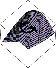
Figure 2: The oriented $2$-patch $M={\bf x}(R)$ is the image of the $2$-square $R=[0,1]\times[0,1]$. The orientation is shown by the curved arrow.

The boundary of $M$ is the $k$-chain

$$\beta(M)={\bf x}(\beta(R))=\oplus_{i=1}^{k}(M^{i}_{+}\oplus M^{i}_{-})$$

where the faces $M^{i}_{\pm}={\bf x}(R^{i}_{\pm})$, respectively, for $i=1,\dots,k$. The tangent vectors $\{{\bf x}_{i}\}_{i=1}^{k}$ at a point ${\bf x}\in M$, defined by

$${\bf x}_{i}=\frac{\partial{\bf x}}{\partial s^{i}},\qquad i=1,\dots,k,$$ (3)

make up a local basis of the tangent space at the point ${\bf x}\in M$, and for a proper, regular patch they are linearly independent and continuous on $M$.

The tangent $k$-vector ${\bf x}_{(k)}$ at a point ${\bf x}\in M$ is the defined by

$${\bf x}_{(k)}={\bf x}_{1}\wedge\cdots\wedge{\bf x}_{k},$$ (4)

and for a proper, regular patch is continuous and doesn’t vanish at any point ${\bf x}\in M$. The reciprocal basis $\{{\bf x}^{i}\}_{i=1}^{k}$ to $\{{\bf x}_{i}\}_{i=1}^{k}$ at the point ${\bf x}\in M$ is defined by

$${\bf x}^{i}=(-1)^{i-1}(\wedge_{j=1,j\neq i}^{k}{\bf x}_{i})\cdot{\bf x}_{(k)}^{-1}$$

and satisfies the relations ${\bf x}^{i}\cdot{\bf x}_{j}=\delta^{i}_{\ j}$. For example for $i=1$,

$${\bf x}^{1}=({\bf x}_{2}\wedge\cdots\wedge{\bf x}_{k})\cdot{\bf x}_{(k)}^{-1}.$$

The oriented tangent $(k-1)$-vector on each face $M^{i}_{\pm}$ of the boundary of $M$ is defined by

$${\bf x}_{(k-1)}=\pm{\bf x}_{(k)}{\bf x}^{i},$$ (5)

respectively. The vector ${\bf x}^{i}$ is reciprocal to ${\bf x}_{i}$, and $\pm{\bf x}^{i}$ defines the directions of the outward normals to the faces $M^{i}_{\pm}$ at the points ${\bf x}\in M^{i}_{\pm}$, respectively.

Let $f,g\colon M\to{\cal G}_{n}$ be continuous ${\cal G}_{n}$-valued functions on the patch $M\subset{\cal M}\subset I\!\!R^{n}$. More precisely, we should define $f$ and $g$ to be continuous on an open set ${\cal S}$ such that $M\subset{\cal S}\subset{\cal M}$, since we will later want $f$ and $g$ to be defined on an open set containing all of $\cal M$.

Definition: The directed integral over $M$ is defined by

$$\int_{M}gd{\bf x}_{(k)}f=\int_{R}g{\bf x}_{(k)}fds^{(k)},$$ (6)

where $ds^{(k)}=ds^{1}\cdots ds^{k}$. We also write $\frac{d{\bf x}_{(k)}}{ds^{(k)}}=\frac{\partial{\bf x}}{\partial s^{1}}\wedge\cdots\wedge\frac{\partial{\bf x}}{\partial s^{k}}$.

Definition: The directed integral over the boundary is

$$\int_{\beta(M)}gd{\bf x}_{(k-1)}f=\sum_{i=1}^{n}\int_{M^{i}_{+}\oplus M^{i}_{-}}gd{\bf x}_{(k-1)}f$$

$$=\sum_{i=1}^{n}\int_{R^{i}_{+}\oplus R_{i}^{-}}g{\bf x}_{(k-1)}fds^{(k-1)}$$

where $ds^{(k-1)}=\frac{ds^{(k)}}{ds^{i}}=ds^{1}\cdots\widehat{d}s^{i}\cdots ds^{k}$ in $R^{i}_{\pm}$.

The directed content of $M$ is defined by

$${\cal D}(M)=\int_{M}d{\bf x}_{(k)}$$

A direct consequence of the fundamental theorem will be that

$${\cal D}(\beta(M))=0.$$

The two sided vector derivative $g({\bf x})\partial_{\bf x}f({\bf x})$ of $f({\bf x})$ and $g({\bf x})$ on $M={\bf x}(r)$ at the point ${\bf x}\in M$ is defined indirectly by

$$g({\bf x})\partial_{\bf x}f({\bf x})=\sum_{i=1}^{k}({\bf x}_{i}\cdot\partial_{\bf x})(\dot{g}{\bf x}^{i}\dot{f})=\sum_{i=1}^{k}\frac{\partial}{\partial s^{i}}(\dot{g}{\bf x}^{i}\dot{f}),$$ (7)

where the deriviatives act only on the dotted arguments. Note in the above definition that we are using the chain rule

$$\partial=\sum_{i=1}^{k}{\bf x}^{i}\frac{\partial{\bf x}}{\partial s^{i}}\cdot\partial_{\bf x}=\sum_{i=1}^{k}{\bf x}^{i}\frac{\partial}{\partial s^{i}}.$$

It follows that the reciprocal vectors ${\bf x}^{i}$ can be expressed in terms of the vector derivative by ${\bf x}^{i}=\partial s^{i}$ for $i=1,\cdots,k$. The Libnitz product rule for partial derivatives gives

$$g\partial f=\dot{g}\partial f+g\partial\dot{f}.$$

Lemma: Let $M$ be a rectangular $k$-patch of class $C^{2}$ in $I\!\!R^{n}$. Then

$$\sum_{i=1}^{j}\frac{\partial}{\partial s^{i}}{\bf x}_{(j)}\cdot{\bf x}^{i}=0,$$

for $j=1,\ldots,k$. In the case when $j=k$, the $``\cdot"$ can be removed.

Proof: For $j=1$, clearly $\frac{\partial}{\partial s^{1}}{\bf x}_{1}\cdot{\bf x}^{1}=\frac{\partial}{\partial s^{1}}1=0$. We now inductively assume that the lemma is true for all $j<k$, and calculate

$$\sum_{i=1}^{k}\frac{\partial}{\partial s^{i}}{\bf x}_{(k)}\cdot{\bf x}^{i}=\sum_{i=1}^{k}\frac{\partial}{\partial s^{i}}[({\bf x}_{(k-1)}\wedge{\bf x}_{k})\cdot{\bf x}^{i}]$$

$$=\frac{\partial}{\partial s^{k}}{\bf x}_{(k-1)}-\sum_{i=1}^{k-1}\frac{\partial}{\partial s^{i}}[({\bf x}_{(k-1)}\cdot{\bf x}^{i})\wedge{\bf x}_{k}]$$

$$={\bf x}_{(k-1),k}-\sum_{i=1}^{k-1}({\bf x}_{(k-1)}\cdot{\bf x}^{i})\wedge{\bf x}_{k,i}=0.$$

In the last step, we have used the fact that partial derivatives commute so that

$${\bf x}_{k,i}=\frac{\partial{\bf x}_{k}}{\partial s^{i}}=\frac{\partial{\bf x}_{i}}{\partial s^{k}}={\bf x}_{i,k}.$$

Theorem[Fundamental Theorem] Let $M$ be a rectangular $k$-patch of class $C^{2}$, and $f,g\colon M\to{\cal G}_{n}$ of class $C^{1}$. Then

$$\int_{M}gd{\bf x}_{(k)}\partial f=\int_{\beta(M)}gd{\bf x}_{(k-1)}f$$ (8)

Proof:

$$\int_{\beta(M)}gd{\bf x}_{(k-1)}f=$$

$$=\sum_{i=1}^{k}\int_{M^{i}_{+}\oplus M^{i}_{-}}gd{\bf x}_{(k-1)}f=\sum_{i=1}^{n}\int_{R^{i}_{+}\oplus R^{i}_{-}}g{\bf x}_{(k-1)}fds^{(k-1)}$$

$$=\sum_{i=1}^{n}\int_{R^{i}_{+}\oplus R_{i}^{-}}\Big{[}\int_{a_{i}}^{b_{i}}\frac{\partial}{\partial s^{i}}(g{\bf x}_{(k)}{\bf x}^{i}f)ds^{i}\Big{]}\frac{ds^{(k)}}{ds^{i}}$$

$$=\sum_{i=1}^{n}\int_{R}\Big{[}\frac{\partial}{\partial s^{i}}(\dot{g}{\bf x}_{(k)}{\bf x}^{i}\dot{f})\Big{]}ds^{(k)}$$

$$=\sum_{i=1}^{k}\int_{M}({\bf x}_{i}\cdot\partial)\dot{g}{d{\bf x}}_{(k)}{{\bf x}^{i}}\dot{f}=\int_{M}gd{\bf x}_{(k)}\partial f.$$

Choosing $g=f=1$, the constant functions, in the Fundamental Theorem immediately gives

Corollary Let $M$ be a rectangular $k$-patch of class $C^{2}$, then

$${\cal D}(M)=\int_{\beta(M)}d{\bf x}_{(k-1)}=0.$$

The fundamental theorem can now be easily extended in the usual way to any simple $k$-surface ${\cal S}$ in $\cal M$ obtained by glueing together $k$-rectangular blocks, making sure that proper orientations are respected on their boundaries.

Classical theorems of integration

Let ${\bf x}(s)$, for $s\in M=[a,b]$ be a $1$-dimensional curve on the $C^{2}$ surface $\cal M$, and let $f,g$ be $C^{1}$ functions mapping $M\to{\cal G}_{n}$. Then the fundamental theorem gives

$$\int_{M}gd{\bf x}\cdot\partial f=\int_{\beta(M)}gd{\bf x}_{(0)}f=g({\bf b})f({\bf b})-g({\bf a})f({\bf a}),$$

where ${\bf a}={\bf x}(a)$ and ${\bf b}={\bf x}(b)$. Of course, this gives the condition of when the integral along a curve connecting the points ${\bf a},{\bf b}\in{\cal M}$ is independent of the path. Note that the vector derivative differentiates both to the left and to the right.

For a $2$-dimensional simple surface ${\cal S}$ embedded in a higher dimensional $k$-manifold ${\cal M}$, with boundary $\beta({\cal S})$, the fundamental theorem gives

$$\int_{\cal S}gd{\bf x}_{(2)}\cdot\partial f=\int_{\beta({\cal S})}gd{\bf x}f.$$ (9)

This is a general integration theorem that includes the classical Green’s theorem in the plane and Stokes’ theorem, among many others, as special cases [15]. If ${\cal M}=I\!\!R^{2}$, then the $2$-surface ${\cal S}$ lies in the plane, and the fundamental theorem (9) takes the form

$$\int_{\cal S}gd{\bf x}_{(2)}\partial f=\int_{\beta({\cal S})}gd{\bf x}f.$$

Choosing $g({\bf x})=1$ and $f=f({\bf x})$ to be a $C^{1}$ vector-valued function, and identifying scalar and bivector parts of the last equation, gives

$$\int_{\cal S}d{\bf x}_{(2)}\partial\wedge f=\int_{\beta({\cal S})}d{\bf x}\cdot f\ \ {\rm and}\ \ \int_{\cal S}d{\bf x}_{(2)}\partial\cdot f=\int_{\beta({\cal S})}d{\bf x}\wedge f,$$

or, equivalently

$$\int_{\cal S}d{\bf x}_{(2)}\partial\wedge f=\int_{\beta({\cal S})}d{\bf x}\cdot f\ \ {\rm and}\ \ \int_{\cal S}d{\bf x}_{(2)}\partial\cdot f=\int_{\beta({\cal S})}d{\bf x}\wedge f,$$

which are two quite different forms of the standard Green’s Theorem [15, p. 110].

If ${\cal S}$ is a simple $2$-surface in ${\cal M}=I\!\!R^{3}$ having the simple closed curve $\beta({\cal S})$ as boundary, then taking the scalar parts of (9), and utilizing the cross product of standard vector analysis, gives

$$\int_{\cal S}(\partial\times f)\cdot\hat{\bf n}|d{\bf x}_{(2)}|=\int_{\beta({\cal S})}f\cdot d{\bf x}$$

which is Stokes’ Theorem. $g=1$ and $f=f({\bf x})$ is a vector-valued function, then the above integral becomes equivalent to the Stokes’ Theorem for a simple surface in $I\!\!R^{3}$.

If ${\cal S}$ is a simple closed $2$-surface in ${\cal M}=I\!\!R^{3}$, $g=1$ and $f=f({\bf x})$ is a vector-valued function, then the fundamental theorem gives

$$\int_{\cal S}d{\bf x}_{(3)}\partial\cdot f=\int_{\beta({\cal S})}d{\bf x}_{(2)}\wedge f,$$

which is equivalent to the Gauss’ Divergence Theorem. This becomes more evident when we multiply both sides of this integral equation by $I^{-1}={\bf e}_{321}$, giving

$$\int_{\cal S}\partial\cdot f\ |d{\bf x}_{(3)}|=\int_{\beta({\cal S})}\hat{\bf n}\cdot f\ |d{\bf x}_{(2)}|,$$

where $\hat{\bf n}$ is the unit outward normal to the surface element $d{\bf x}_{(2)}$ at the point ${\bf x}\in\beta({\cal S})$. There are many other forms of the classical integration theorems, and all of them follow directly from our fundamental theorem.

Over the last several decades a powerful geometric analysis has been developed in geometric algebra. One of the most striking features of this new theory is the generalization of the concept of an analytic function to that of a monogenic function [16].

Definition: A geometric-valued $C^{1}$ function $f({\bf x})$ is said to be monogenic on ${\cal S}\subset{\cal M}$ if $\partial_{\bf x}f=0$ for all ${\bf x}\in{\cal S}$.

Let ${\cal M}=I\!\!R^{n}$ and let $\cal S$ be the $(n-1)$-dimensional simple closed boundary containing an open region $M$ of $\cal M$. Let $f=f({\bf x})$ be a $C^{1}$ geometric-valued function defined on $M$ and its boundary ${\cal S}$. Then for any point ${\bf x}^{\prime}\in M$,

$$f({\bf x}^{\prime})=\frac{1}{\Omega}\int_{M}|d{\bf x}_{(n)}|\frac{({\bf x}^{\prime}-{\bf x})}{|{\bf x}^{\prime}-{\bf x}|^{n}}\partial_{{\bf x}}f({\bf x})-\frac{1}{\Omega}\int_{\cal S}|d{\bf x}_{(n-1)}|\frac{({\bf x}^{\prime}-{\bf x})}{|{\bf x}^{\prime}-{\bf x}|^{n}}\hat{\bf n}f({\bf x}),$$

where $\hat{\bf n}$ is the unit outward normal to the surface ${\cal S}$ and $\Omega=\frac{2\pi^{n/2}}{\Gamma(n/2)}$ is the area of the $(n-1)$-dimensional unit sphere in $I\!\!R^{n}$. This important result is an easy consequence of the fundamental theorem by choosing $g({\bf x})$ to be the Cauchy kernel function $g({\bf x}^{\prime})=\frac{({\bf x}^{\prime}-{\bf x})}{|{\bf x}^{\prime}-{\bf x}|^{n}}$, which has the property that $\partial_{{\bf x}^{\prime}}g({\bf x}^{\prime})=0$ for all ${\bf x}^{\prime}\neq{\bf x}\in I\!\!R^{n}$. For a monogenic function $f({\bf x})$, we see that

$$f({\bf x}^{\prime})=-\frac{1}{\Omega}\int_{\cal S}|d{\bf x}_{(n-1)}|\frac{({\bf x}^{\prime}-{\bf x})}{|{\bf x}^{\prime}-{\bf x}|^{n}}\hat{\bf n}f({\bf x}).$$

This means that a monogenic function $f({\bf x})$ in a region $M\subset I\!\!R^{n}$ is completely determined by its values on its boundary $\cal S$. This, of course, generalizes Cauchy’s famous integral theorem for analytic functions in the complex number plane [17].

The vector derivative in $I\!\!R^{n}$

General formulas for the vector derivative on a $k$-surface would take us deep into differential geometry [12]. Here, we will only give a few formulas for the vector derivative on $I\!\!R^{n}$, which were utilized in the derivation of the generalized Cauchy integral formula given in the last section. The vector derivative $\partial_{\bf x}$ on $I\!\!R^{n}$ can be most simply expressed in terms of the standard basis, $\partial=\partial_{\bf x}=\sum_{i=1}^{n}{\bf e}_{i}\frac{\partial}{\partial x^{i}}$. Where the position vector ${\bf x}\in I\!\!R^{n}$ has the coordinate form

$${\bf x}=(x^{1}\ \cdots\ x^{n})=\sum_{i=1}^{n}x^{i}{\bf e}_{i}.$$

The following formulas are easily verified:

1. $\partial\cdot{\bf x}=n$ and $\partial\wedge{\bf x}=0$, as easily follows from $\partial\ {\bf x}=\partial\cdot{\bf x}+\partial\wedge{\bf x}=n$,

2. ${\bf a}\cdot\partial\ {\bf x}={\bf a}=\partial\ {\bf x}\cdot{\bf a}$, as easily follows from ${\bf a}\cdot(\partial\wedge{\bf x})={\bf a}\cdot\partial\ {\bf x}-\partial\ {\bf x}\cdot{\bf a}=0,$

3. $\partial\ {\bf x}^{2}=\partial\ \dot{\bf x}\cdot{\bf x}+\partial\ {\bf x}\cdot\dot{\bf x}=2{\bf x}$,

4. $\partial|{\bf x}|=\partial({\bf x}^{2})^{1/2}=\frac{1}{2}({\bf x}^{2})^{-1/2}2{\bf x}=\hat{\bf x}$,

5. $\partial|{\bf x}|^{k}=k|{\bf x}|^{k-2}{\bf x}$,

6. $\partial\frac{{\bf x}}{|{\bf x}|^{k}}=\frac{n-k}{|{\bf x}|^{k}}$,

7. $\partial\log|{\bf x}|=\frac{{\bf x}}{|{\bf x}|^{2}}={\bf x}^{-1}$.

References

• [1] D. Hestenes, Multivector Calculus, Journal of Mathematical Analysis and Applications, 24, No. 2, November 1968, 313-325.
• [2] G. Sobczyk, Simplicial Calculus with Geometric Algebra, in Clifford Algebras and Their Applications in Mathematical Physics, Edited by A. Micali, R. Boudet, and J. Helmstetter, (Kluwer Academic Publishers, Dordrecht 1992).
• [3] O.L. Sánchez, Una Transformada de Clifford-Fourier y Teoremas de Tipo Paley-Wiener, Master’s Degree Thesis, Benemérita Universidad Autónoma de Puebla, Puebla, Mexico 2008.
• [4] H. Flanders, Differential Forms with Applications to the Physical Sciences, Dover Publications, 1989.
• [5] W.K. Clifford, Applications of Grassmann’s extensive algebra, Amer. J. of Math. 1 (1878), 350-358.
• [6] M. J. Crowe. A History of Vector Analysis, Chapter 6, Dover 1985.
• [7] R. Sjamaar, Manifolds and Differential forms, Lecture Notes, Cornell University, (http://www.math.cornell.edu/~sjamaar/).
• [8] E. Bayro Corrochano, G. Sobczyk, Editors, Geometric Algebra with Applications in Science and Engineering, Birkhäuser, Boston 2001.
• [9] L. Dorst, C. Doran, J. Lasenby, Editors, Applications of Geometric Algebra in Computer Science and Engineering, Birkhäuser, Boston 2002.
• [10] T. Danzig. Number: The Language of Science, $4^{th}$ Ed., Macmillan, 1954.
• [11] D. J. Struik. A Concise History of Mathematics, Dover, 1967.
• [12] D. Hestenes and G. Sobczyk. Clifford Algebra to Geometric Calculus: A Unified Language for Mathematics and Physics, 2nd edition, Kluwer 1992.
• [13] P. Lounesto. Clifford Algebras and Spinors. Cambridge University Press, Cambridge, 1997.
• [14] http://users.tkk.fi/~ppuska/mirror/Lounesto/ http://modelingnts.la.asu.edu/GC_RD&.html http://www.mrao.cam.ac.uk/~clifford/ http://staff.science.uva.nl/~leo/clifford/
• [15] M. R. Spiegel, Vector Analysis and an introduction to Tensor Analysis, Schaum’s Outline Series, Schaum Publishing Co., New York 1959.
• [16] F. Brackx, R. Delanghe and F. Sommen, Clifford analysis, Research Notes in Mathematics, Vol. 76, Pitman Advanced Publishing Program, Boston 1982.
• [17] L. V. Ahlfors, Complex Analysis, McGraw-Hill Book Company, N.Y. 1979.