Estimating the Parameters of Sgr A*’s Accretion Flow Via Millimeter VLBI
Abstract
Recent millimeter-VLBI observations of Sagittarius A* (Sgr A*) have, for the first time, directly probed distances comparable to the horizon scale of a black hole. This provides unprecedented access to the environment immediately around the horizon of an accreting black hole. We leverage both existing spectral and polarization measurements and our present understanding of accretion theory to produce a suite of generic radiatively inefficient accretion flow (RIAF) models of Sgr A*, which we then fit to these recent millimeter-VLBI observations. We find that if the accretion flow onto Sgr A* is well described by a RIAF model, the orientation and magnitude of the black hole’s spin is constrained to a two-dimensional surface in the spin, inclination, position angle parameter space. For each of these we find the likeliest values and their 1- & 2- errors to be , , and , when the resulting probability distribution is marginalized over the others. The most probable combination is , and , though the uncertainties on these are very strongly correlated, and high probability configurations exist for a variety of inclination angles above and spins below . Nevertheless, this demonstrates the ability millimeter-VLBI observations, even with only a few stations, to significantly constrain the properties of Sgr A*.
Subject headings:
black hole physics — Galaxy: center — techniques: interferometric — submillimeter — accretion, accretion disks1. Introduction
Understanding the structure and dynamics of black hole accretion flows has remained a central problem in astrophysics. Only in the past decade have sufficient numerical resources existed to perform self-consistent, three-dimensional magneto-hydrodynamic (MHD) simulations capable of resolving the magneto-rotational instability, believed to be responsible for angular-momentum transport in black-hole accretion flows. However, a true ab initio computation is still well beyond reach, resulting in the need for a variety of simplifying assumptions (e.g., the suitability of MHD, importance of electron-ion coupling, properties of accelerated electrons, etc.). As a result, the number of applicable models has rapidly proliferated, many of which are capable of describing the variety of phenomena observed. This is due in large part to the inability of current observations to resolve horizon scales. Unfortunately, the compact nature of black holes makes it very difficult to access the inner-edge of black hole accretion flows.
Sagittarius A* (Sgr A*), the bright radio point source coincident with the center of the Milky Way, is presently the best studied known black-hole candidate. Observations of orbiting OB-stars, the closest of which passes within of Sgr A*, have produced a measured mass of and an Earth-Sgr A* distance111The mass and distance measurements are strongly correlated, with mass scaling roughly as . of (Ghez et al. 2009; Gillessen et al. 2008). Already, there is strong evidence for the existence of horizon in this source (Broderick & Narayan 2006; Broderick, Loeb & Narayan 2009). However, in many ways, Sgr A* is very different than the supermassive black holes in AGN. Unlike its active brethren, Sgr A* is vastly under-luminous, with a luminosity many orders of magnitude smaller than the Eddington luminosity. As a result, it is widely expected that Sgr A*’s accretion flow is quite different from those in AGN, though perhaps more indicative of the roughly 90% of supermassive black holes that are not presently in an active phase.
Even when strong-gravitational lensing is accounted for, the apparent angular size of Sgr A*’s horizon is only , a factor of two larger than the next largest black hole (M87) and orders of magnitude larger than any other known black hole (including all stellar-mass black holes). Nevertheless, despite its tiny angular size, recent millimeter VLBI experiments have successfully resolved this scale (Doeleman et al. 2008). Since only three telescopes were involved with these observations, the resulting – coverage of the measured visibilities is very sparse. As a result only two simple models of Sgr A*’s image, a Gaussian and an annulus, were fit to the data by Doeleman et al. (2008).
However, we have a great deal of additional information about Sgr A*, including its spectral and polarization properties. We may also require physical consistency in any model (which would likely rule out an annulus, for example). Furthermore, we would like to evaluate the ability of, and optimize for this purpose, future millimeter and sub-millimeter VLBI experiments to constrain fundamental properties of the accretion flow in Sgr A*. This paper demonstrates the fitting and parameter estimation procedure for a simple radiatively inefficient accretion disk model (RIAF). In particular, we show that even from very sparse baseline coverage it is possible to robustly extract interesting parameters of a generic RIAF. A study that considers how future high frequency VLBI observations can extend this work will be presented elsewhere (Fish et al. 2008).
In the analysis presented here, we make full use of all the observations described in Doeleman et al. (2008). These include two days of VLBI observations at 230GHz that targeted Sgr A* using an array consisting of the James Clerk Maxwell Telescope (JCMT) on Mauna Kea, the Arizona Radio Observatory Submillimeter Telescope (SMTO) on Mt. Graham in Arizona, and one dish of the Coordinated Array for Research in Millimeter-wave Astronomy (CARMA) in California. Robust detections of Sgr A* and correlated flux density measuremnets were obtained on the CARMA-SMTO and JCMT-SMTO baselines. No detections were found on the CARMA-JCMT baseline resulting in upper limits on the correlated flux density. In addition, contemporaneous total flux density measurements at the same frequency were obtained by using the full CARMA array operating as a stand-alone instrument. Full details of the observations, calibration, and data processing can be found in Doeleman et al. (2008).
In section 2 we present the simple accretion flow model that we employ. Sections 3 and 4 discuss the data fitting procedure, including the Bayesian method by which we do the parameter estimation, and the generic constraints placed by the current VLBI results. Section 5 details how we define our uncertainties and presents our parameter estimates. Finally, we conclude in section 6.
2. RIAF Visibility Modeling
2.1. Accretion Flow Modeling
Sgr A* transitions from an inverted, optically thick spectrum to a optically thin spectrum near millimeter wavelengths. This implies that Sgr A* is only becoming optically thin at . Due to relativistic effects this transition does not occur isotropically for orbiting gas (e.g., Broderick & Loeb 2006a), becoming optically thin on the receding side at longer wavelengths than the approaching side of the accretion flows orbit. As a consequence, the opacity of the underlying accretion flow is crucial to imaging Sgr A*’s accretion flow.
Despite being diminutive in comparison to the Eddington luminosity for a black hole, Sgr A* is still considerably bright, emitting a bolometric luminosity of approximately . Thus, it has been widely accepted that Sgr A* must be accretion powered, implying a minimum accretion rate of at least . It is presently unclear how this emission is produced. This is evidence by the variety of models that have been proposed to explain the emission characteristics of Sgr A* (e.g., Narayan et al. 1998; Blandford & Begelman 1999; Falcke & Markoff 2000; Yuan et al. 2002, 2003; Loeb & Waxman 2007). Models in which the emission arises directly from the accreting material have been subsumed into the general class of RIAFs, defined by the generally weak coupling between the electrons, which radiate rapidly, and the ions, which efficiently convert gravitational potential energy into heat (Narayan et al. 1998). This coupling may be sufficiently weak to allow accretion flows substantially in excess of the required to explain the observed luminosity with a canonical radiative efficiency.
Nevertheless, the detection of polarization from Sgr A* above (Aitken et al. 2000; Bower et al. 2001, 2003; Marrone et al. 2006), and subsequent measurements of the Faraday rotation measure (Macquart et al. 2006; Marrone et al. 2007), has implied that the accretion rate near the black hole is significantly less than the Bondi rate, requiring the existence large-scale outflows (Agol 2000; Quataert & Gruzinov 2000). Therefore, in the absence of an unambiguous theory, we adopt a simple, self-similar model for the underlying accretion flow which includes substantial mass-loss.
For concreteness, as in Broderick & Loeb (2006a), we follow Yuan et al. (2003), and employ a model in which the accretion flow has a Keplerian velocity distribution, a population of thermal electrons with density and temperature
| (1) |
and
| (2) |
respectively, a population of non-thermal electrons
| (3) |
and a toroidal magnetic field in approximate () equipartition with the ions (which produce the majority of the pressure), i.e.,
| (4) |
In all of these, is the Schwarschild radius, is the cylindrical radius and is the vertical coordinate. Inside of the innermost-stable circular orbit (ISCO) we assume the gas is plunging upon ballistic trajectories. In all of these expressions the radial structure was taken directly from Yuan et al. (2003) and the vertical structure was determined by assuming the disk height is comparable to . Given a choice for the coefficients and a radiative transfer model, images may then produced using the fully-relativistic ray-tracing and radiative transfer schemes described in Broderick & Loeb (2006a) and Broderick & Loeb (2006b).
The primary emission mechanism is synchrotron, arising from both the thermal and non-thermal electrons. We model the emission from the thermal electrons using the emissivity described in Yuan et al. (2003), appropriately altered to account for relativistic effects (see, e.g., Broderick & Blandford 2004). Since we perform polarized radiative transfer via the entire complement of Stokes parameters, we employ the polarization fraction for thermal synchrotron as derived in Petrosian & McTiernan (1983). In doing so we have implicitly assumed that the emission due to thermal electrons is isotropic, which while generally not the case is unlikely to change our results significantly. For the non-thermal electrons we follow Jones & O’Dell (1977) for a power-law electron distribution, cutting the electron distribution off below a Lorentz factor of and corresponding to a spectral index of , both roughly in agreement with the assumptions in Yuan et al. (2003). For both the thermal and non-thermal electrons the absorption coefficients are be determined directly via Kirchoff’s law.
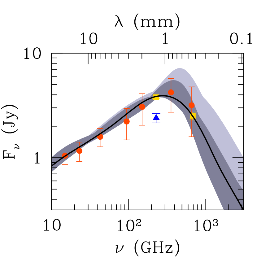
As in Broderick & Loeb (2006a), to correct for the fact that Yuan et al. (2003) was a Newtonian study, the three coefficients (, and ) were adjusted to fit the average radio, sub-millimeter and near-infrared spectrum of Sgr A*. However, our procedure is different from that employed in Broderick & Loeb (2006a) in two respects. Firstly, we keep the radial index of the non-thermal electrons fixed for all models. Secondly, the fitting is performed systematically for a large number of positions in the inclination–spin parameter space, yielding a tabulated set of coefficient values. For every inclination and black hole spin presented here this was possible with extraordinary accuracy (reduce in all cases and for many), implying that this model is presently significantly under-constrained by the quiescent spectrum alone222Part of the reason for this is almost certainly the fact that many of the radio fluxes were measured during different observational epochs, and thus the flux uncertainties are indicative of the source variability, not the intrinsic measurement error. For two of the data points in Fig. 1 (the yellow squares), this is not the case, having been measured coincidentally, and thus these play a much more significant role in constraining the RIAF model parameters.. Subsequently, we obtained the appropriate model parameters for arbitrary spins and inclinations via a high-order polynomial interpolation.
The range of spectra for the models we employ here is presented in Fig. 1, together with the radio & sub-millimeter data that was used for the fitting procedure. The shown spectra deviate from the fitted spectra much more significantly than the scatter in the fitted spectra themselves. This is due almost entirely to interpolation process, and is most extreme at high-spins, where the coefficient values begin to change rapidly (and thus have larger interpolation errors). Nevertheless, these do not produce substantially different images at from their tabulated counterparts, and it is important to note that the associated error in the underlying RIAF model serves only to favor very high spins (), since in these cases it results in a larger accretion-flow photosphere and, as we shall see, the small size of the photosphere of the high-spin models is the primary reason they are excluded. Hence, in reality, such models are more strongly disfavored than shown here. All of these models are also capable of producing the Faraday rotation measures observed, and thus the polarimetric properties of Sgr A*.
At the time that Sgr A* was being monitored by Doeleman et al. (2008) it exhibited an anomalously low flux of , almost below its average value (shown by the blue triangle in Fig. 1). To appropriately account for this we chose a “minimal” prescription for changing the model, reducing all densities by a fixed factor (decreasing the magnetic field such that is fixed) until the observed flux was reproduced. In a sense, this models the low flux as a low-mass accretion period. These lower-density models do have noticeably smaller, though qualitatively similar, images compared to those used in the spectral fits.
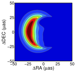
An example image is shown in the left-panel of Fig. 2 for a moderate spin and viewing inclination. As seen in previous efforts to image relativistic accretion flows, the flow appears as a crescent associated with the approaching side of the accretion disk (Broderick & Loeb 2006a, b). The non-negligible optical depth obscures the black hole “silhouette” on this side. The receding side is all but invisible as a consequence of the Doppler shift and Doppler beaming associated with the relativistic orbital motion in the inner-most portions of the accretion flow. Images for are related by a reflection (across a line perpendicular to the projected spin axis) to images with an inclination . However, due to the approximate reflection symmetry of the RIAF model images, the constraints arising from spins pointed counter to and along the line of sight are nearly identical. As a result, for clarity we restrict ourselves to the latter range.
Using this model we created a library of ideal-resolution images, each with a flux of , having different spins and viewing inclinations spanning all possible values.
2.2. Interstellar Electron Scattering
The existence of an interstellar scattering screen between Earth and the Galactic center has been well known for some time now. This has been carefully characterized empirically by a number of authors; we use the recent model from Bower et al. (2006). In this the observed flux distribution is obtained by convolving the ideal flux with an anisotropic Gaussian scattering kernel. The anisotropic Gaussian is defined by the scattering widths along major and minor axes (both ) and the position angle of the minor axis (which is independent of ). From Bower et al. (2006), the associated full-width, half-max for the major and minor axes are
| (5) | |||||
| (6) |
with the major axis oriented East of North. In practice, the broadening was done in the – plane, where it reduces to a multiplicative factor.

2.3. Visibility Modeling
Visibilities are then defined in the normal way:
| (7) |
where are the intensities on the image plane, with aligned East-West and North-South. Because changing the position angle, (vanishing at North and increasing towards the East), corresponds simply to a coordinate rotation, the images were originally computed only for a single position angle, namely . The visibilities associated with the ideal-resolution images were then computed, and subsequently rotated to the desired . In practice, the visibilities were calculated via a Fast Fourrier Transform, which was padded sufficiently to resolve the shortest baseline (SMTO-CARMA). We also vary the total flux, or equivalently . For sufficiently different values a new image must be produced. However, for small variations around our canonical value of (within ) simply renormalizing the visibilities produces a good approximation. Finally, the interstellar-scatter broadening was effected by multiplying the visibilities in the – plane by the Fourier-transformed scattering kernel.
Since Sgr A* was detected on only two of the three VLBI stations, there was insufficient observational data to determine the individual baseline visibility phases. Thus, henceforth, by visibility (and ) we shall, more properly, refer to the visibility magnitudes. These are necessarily a function of position in the – plane, black hole spin (), spin inclination (), position angle of the projected spin vector () and flux normalization (). That is, for a particular realization of the RIAF model, we have computed .
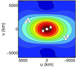
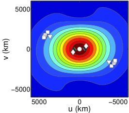
The ideal and broadened visibilities are shown in the center and right-panels of Fig. 2, respectively. In both of these the positions of the observed visibilities are shown by the white points. As expected, associated with the narrow-axis of the image crescent is a correspondingly broad feature in the visibilities. On the maximum scale of interest (the JCMT-SMTO baseline) the power is not substantially reduced by the interstellar electron scattering. At the same time, along the long-axis of the image crescent the visibilities drop off rapidly. Thus, we may expect that, at the very least, the VLBI observations will constrain . This turns out to be correct.
3. Bayesian Data Analysis
We follow a Bayesian scheme to compute the probability that given the measured visibilities, a given set of model parameters (,,) are correct. This is, of course, predicated upon the assumption that our simplistic RIAF model is appropriate for Sgr A*. Indeed, this is the primary uncertainty in our reported constraints upon , and . While we can address this model dependence somewhat by comparing the results from different black hole masses, at this point we can only hope that our results are characteristic of generic RIAF models. This is not unreasonable given that the primary physics responsible for the structure of our images, the Keplerian velocity profile, is a common theme among RIAF models. Nevertheless, it remains to be proven.
Assuming the observational errors are Gaussian, the probability of measuring a visibility given a particular set of model parameters is
This is appropriate for detections, i.e., along the SMTO-CARMA and JCMT-SMTO baselines. However, for the non-detection associated with the CARMA-JCMT baseline this is not the case. As discused in Appendix A, the probability of a non-detection given a measurement threshold of and intrinsic uncertainty of and expected value is
Therefore, the probability of observing the measured set of independent visibilities given a particular RIAF model is
| (8) | |||||
where the first product is over the detections on the SMTO-CARMA (SC) and JCMT-SMTO (JS) baselines, and the second is over the non-detections on the CARMA-JCMT (CJ).
In order to assess the quality of the modeling at each spin and inclination, we appeal to the Bayesian Information Criterion (). Specifically,
| (9) |
where is the number of parameters and is the number of data points. In the absence of the non-detection, this reduces to the normal definition of , up to an additive constant, and thus comparing models with similar numbers of parameters reduces to the normal minimization. Since this latter statistic is commonly used, and its properties generally well known, solely for the purpose of assessing the quality of the fits we define an effective :
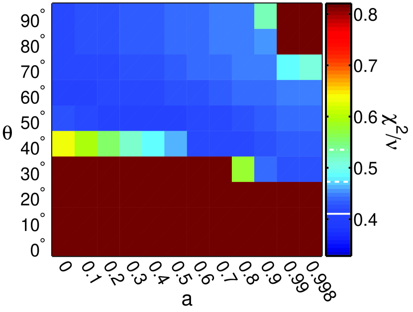
Note that since only one of the visibility measurements is an upper limit, we may expect that this definition of will behave very similarly to the standard definition in our case. The reduced effective is shown as a function of spin and inclination in Fig. 3 for the best fit and . For nearly all inclinations above a good fit can be found (indeed, !). The exception is at very high spins and high inclinations (where the disk is edge on)333Note that in this procedure we have ignored the statistics associated with fitting the spectrum, choosing to break up these two components of the fitting process to stress the implications of the new millimeter VLBI observations..
While eq. (8) gives the probability that the observed visibilities come from a given model, what we would like to know is somewhat different: the probability of a set of model parameters given the observed visibilities. That is, we would like the probability density . With an appropriate choice of priors on , , and , we may construct the desired probabilities via Bayes’ theorem. As such, we now turn to the problem of choosing these priors.
A natural choice for the prior upon and comes from the assumption that Sgr A*’s spin orientation probability is isotropic, i.e., we have no other information regarding its direction. This results in . In the absence of a complete theoretical understanding of the spin evolution of supermassive black holes, we choose the prior on to be uniform, i.e. . Finally, we set the prior on to be uniform as well. Since the allowed range of variation in is small, and the prior probability is expected to vary smoothly, this is not a significant oversight. Therefore, Bayes’ theorem gives
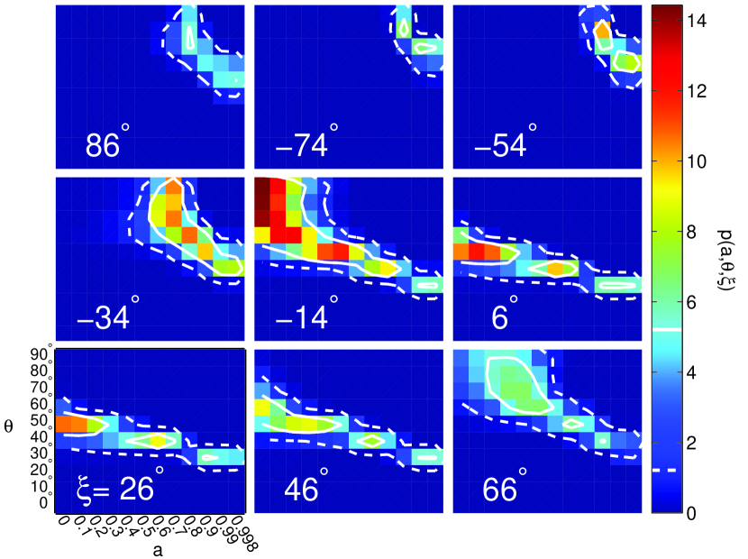
This is necessarily a probability density in a four-dimensional parameter space, and thus is quite difficult to visualize directly. Furthermore, some of these parameters are physically more interesting than others. Therefore, we construct a variety of marginalized probabilities from this for presentation and analysis. The most general is simply marginalized over :
| (11) |
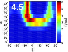
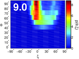
This probability distribution is shown explicitly in Fig. 6. We construct a pair of two-dimensional marginalized probability densities as well:
| (12) |
and
| (13) |
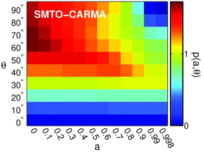
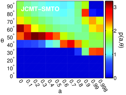
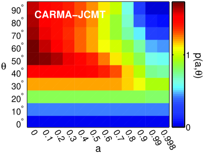
These are plotted in Fig.’s 4 and 5. Alternatively, we could choose the most likely values of either or . For some of the panels in Fig. 4, we choose a hybrid probability: marginalized over but the most likely in . Finally, for the purpose of identifying the probability distribution of each parameter separately, we also construct the marginalized one-dimensional probability densities:
| (14) | |||||
| (15) | |||||
| (16) |
These are shown in Fig 7.
4. The Nature of the VLBI Constraints
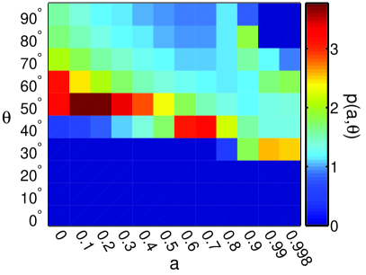
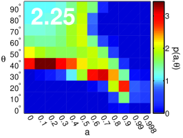
The relative importance of the three different baselines is shown in Fig. 4. To make a direct comparison of the contributions from different baselines possible, the top-left, top-right and bottom-left panels of Fig. 4 show the probability after setting to the most likely value and marginalizing over (justified by the fact that the probability distributions in are quite similar, while those in were not). Both the SMTO-CARMA detections and the CARMA-JCMT upper limit exclude the high-spin, high-inclination portion of the parameter space. This is primarily because high-spin RIAF models result in images that are sufficiently compact to substantially over-predict the flux observed on both of these baselines. Due to its considerably longer baseline length, the CARMA-JCMT non-detection is more constraining than the multiple SMTO-CARMA detections, despite only representing an upper-limit.
As anticipated, most constraining are the visibilities measured on the JCMT-SMTO baseline. This baseline convincingly excludes low inclinations (face-on disks). This may be easily understood, qualitatively, in terms of the RIAF images themselves. As inclination increases, the RIAF image becomes more asymmetric, and increasingly dominated by a thin crescent (e.g., left-panel of Fig. 2). It is generally the direction across the minor-axis of the crescent that has the shortest scale intensity variations, and consequently determines the long-baseline visibilities. Below a critical inclination, the crescent grows sufficiently fat that it is resolved out by the JCMT-SMTO baseline.
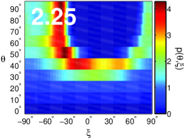
At large inclinations, the crescent becomes too thin, requiring the JCMT-SMTO baseline to be oriented obliquely relative to the spin axis of Sgr A*. This restricts the available values of to an increasingly limited range, as may be seen explicitly in the bottom-center panel of Fig. 5. Thus, while it is nearly always possible to obtain a satisfactory fit, the reduced range in position angle makes such a configuration unlikely. Hence we find that the long-baseline visibilities strongly constrain the possible values of inclination and spin to a narrow band near and generally favoring moderate . We note that the appearance of islands of high probability in the top-right panel of Fig. 4 is almost certainly due to under sampling in near this critical region, and not indicative of a bifurcation in the allowed parameter space.
This behavior is clearly visible in the combined , which closely resembles that from the JCMT-SMTO baseline alone. In this case, we have marginalized over as well as (i.e., as defined by eq. 12), though the difference had we chosen the most likely value of is less than 10% everywhere. The shorter baselines have effectively removed a small high-spin, high-inclination island that persisted in the JCMT-SMTO probability distribution alone. Additionally, they have further restricted the spin to low-to-moderate levels. The combined result, however, is to restrict the spin and inclination to a narrow strip.
In a similar fashion, appears to limit RIAF models to a narrow band of orientations. Due to the approximate up-down symmetry of the image (parallel to the projected spin axis), the corresponding band has a characteristic “U” shape, corresponding to something akin to a taco shell in the ,, parameter space. (Note that we do not plot over the entire range due to the symmetry of the visibilities under reflection.)
In order to ascertain how the present uncertainty in the mass of Sgr A* effects our conclusions, we repeated the analysis for black hole masses of and . Since the mass uncertainty is strongly correlated with the distance to Sgr A* ( is very well determined by stellar orbits, Ghez et al. 2009; Gillessen et al. 2008), we altered the distance to the Galactic center accordingly. As a consequence, the roughly 10% change in the mass results in a 4% change in the angular scale of the RIAF images. A correspondingly small change was seen in the resulting probability distributions, implying that, apart from the the RIAF modeling, the paucity of millimeter-VLBI observations is the dominant obstacle to constraining the black hole spin properties.
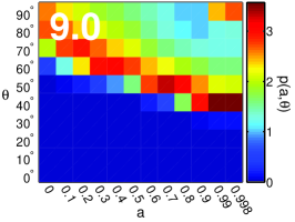
Altering the angular scale of the images also provides a proxy, albeit a poor one, for considering different Sgr A* models, corresponding to different disk scale lengths. and for a black holes of mass and are compared to those determined using the estimated value of in Fig. 5. These extreme mass changes correspond to a 30% change in the angular scales of the images, and can make a substantial difference to the resulting probability distributions. Nevertheless, high inclinations and low spins are still generally preferred, though less so for large images.
Finally, because Sgr A* is an inherently dynamical environment, exhibiting substantial variations in the millimeter flux on time scales, we may not be justified in assuming that the image of Sgr A* was stationary during the entire time that observations were made. Indeed, searching for variations in the VLBI closure quantities has been suggested as a way to directly probe the existence of hot spots in Sgr A*’s accretion flow (Doeleman et al. 2008). Therefore, to check this, we repeated this analysis for the two days over which the observations were performed separately, finding no significant difference. This implies that either Sgr A* was quiescent during this time or that the individual observation windows were sufficiently long to average out this activity. The anomalously low flux suggests the former interpretation is correct.
5. Parameter Estimation
It is evident from the previous section that the allowed parameter space is highly non-Gaussian. As such, we must take special care in how we extract values and their attendent uncertainties for the fitting parmeters. In all cases, these values will be highly correlated, and the systematic uncertainties due to the choice of a particular RIAF model will dominate the errors (and thus will not be reviewed again in this section).
In order to determine - and - error surfaces, we first define a cumulative probability
| (17) |
where are the parameters of the total probability distribution. That is, is simply the probability associated with the region of the parameter space that has probability density above . This is necessarily a monotonic function of , which may then be inverted to find as a function of . We then define the - contour to be that associated with the for which . Similarly, we define the - contour by . While these satisfy the normal definition of - and - errors, it is important to remember that in our case the errors are strongly non-Gaussian.
Fig. 6 shows the probability density in the full three-dimensional parameter space as a sequence of constant- slices. The most likely parameter combination is , and . However, as remarked in the previous section, there are acceptable solutions for a wide range of , and . The primary effect of the VLBI measurements is to restrict these parameters to a band around a two-dimensional surface, resembling a taco shell with its sides around and , the highest probability densities clustered on the former. Generally, we see a preference for low spins and can rule out inclinations below .
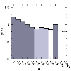
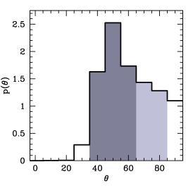
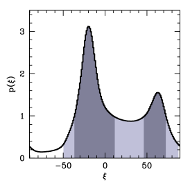
More diagnostic for single parameters are the fully marginalized probability distributions shown in Fig. 7. It must be remembered, however, that these parameter estimates are strongly correlated, and thus these estimates should be used with caution. Again we use the cumulative probability, to define the - and - surfaces, shown in the panels of Fig. 7 as the dark and light shaded regions, respectively.
From the left panel of Fig. 7, the most likely spin is . While we can rule out very high spins () at the - level for our particular RIAF model, the spin is otherwise weakly constrained. Moreover, it appears to have a small high-spin island, at the - level, around . The presence of this island is limited by the CARMA-JCMT non-detection, and therefore can be directly probed via future observations.
In contrast, the inclination is fairly robustly limited. The most likely inclination is , where the lopsided errors are due to the lopsided nature of the probability distribution. It is very clear in the center panel of Fig. 7 that face-on geometries () are convincingly ruled out. However, there is a tail extending to higher inclinations444Indeed, as mentioned above, the most likely overall set of parameters has ..
The distribution of position angles is more complicated than either spin or inclination. In the right panel of Fig. 7 we see the taco-shell geometry most clearly in terms of the bimodal distribution of likely . The most probable position angle is . However, a second solution does exist at , though containing only of the probability (under the - peak) of the more likely solution.
Our limits upon the inclination are in quite good agreement with previous efforts. Huang et al. (2007) fit a qualitatively different RIAF model, primarily neglecting orbital motion, at and . While these favor high inclinations, the fact that the images are dominated by interstellar scattering prevents a conclusive measurement. Similarly, efforts to fit Sgr A*’s flares with hydrodynamic instabilities find an inclination of roughly , though the systematic uncertainty associated with their model is unclear. Fitting a qualitatively different model to the long-wavelength observations, a hydrodynamic jet, Markoff et al. (2007) also favor large inclinations (). However, it is not obvious how this qualitative agreement should be interpreted, given the very different geometries involved.
Unlike the inclination, our position angle estimate disagrees significantly with many previous efforts. The primary solution is in good agreement with the and fits of RIAF models by Huang et al. (2007), which imply . While there is considerable uncertainty in their estimates (like ours), we note that their result is not consistent with our second solution at the 1- level. In contrast, only our second solution is in agreement with analyses of NIR polarization observations, assuming a simplistic orbiting hot-spot model, which find (Meyer et al. 2007). This is not particularly surprising given the difficulties in assessing the relationship between the emitted polarization and the underlying plasma geometry. At the 1- level, none of our solutions are consistent with efforts to fit jet models to Sgr A* at , which find (Markoff et al. 2007). This is also not unexpected given the considerably different geometries involved. Between all of these (even prior to our estimate), nearly all values of have been reported, suggesting that significant improvements in theoretical understanding and additional observations are required before this question can be settled.
Finally, note that our estimates imply that the X-ray feature described in Muno et al. (2008) is not associated with a putative jet, but simply another filamentary structure in the vicinity of Sgr A*. However, interestingly, our primary position angle estimate (and that of Huang et al. 2007) is similar to the orientation of the compact, clockwise disk of massive stars orbiting the Galactic center (Genzel et al. 2003). This is somewhat surprising given the the large radii () of the stellar disk, though may be natural if the observed stars are the remnants of an active period in Sgr A*’s recent past.
6. Conclusions
Despite the sparse – coverage, and the existence of a detection on only one long baseline, we have been able to significantly constrain the possible parameters of an accretion flow onto Sgr A*. Within the context of a qualitative RIAF model that fits the observed spectra of Sgr A*, we have have been able to substantially constrain the orientation of Sgr A*’s spin. The magnitude of this spin is less well determined, though the black hole cannot be maximally rotating. This result is relatively insensitive to the black hole mass.
We have not ascertained the strength of our constraints’ dependence upon the particular RIAF model, though our estimates are consistent with earlier efforts comparing longer wavelength observations to an alternative RIAF model. However, there are two additional reasons to believe that our results will be generic of RIAF models. The first is that the underlying physics that limits the orientation is the Doppler beaming and boosting that is dependent primarily upon the Keplerian velocity profile of the accretion flow, a feature that is generic among RIAF models. The second is the weak dependence upon large variations in mass, implying that changing the scale lengths of the accretion model does little to alter our results. Thus, we expect the qualitative form of our constraints to be a generic feature of all RIAF models for Sgr A*, and our quantitative results to be roughly correct. Of course, should the emission observed from Sgr A* not arise in an accretion flow, our results could be quite different.
As implied by the right-panel of Fig. 2, additional long-baseline observations are sorely needed to unambiguously determine both the applicability of RIAFs to Sgr A* and constrain their parameters. In a companion paper, Fish et al. (2008) we report upon an analysis of the ability of possible millimeter VLBI arrays to do so. Given the number of potential radio telescopes that could be added to the current VLBI array (Doeleman et al. 2008), the prospects for making significant progress in model parameter estimation are excellent. Already it is clear that with the advent of millimeter VLBI we are now entering an era of precision black-hole accretion physics.
Appendix A Non-detection Probability
Consider an observable , with an expected value of and Gaussian random errors of amplitude . Then, the probability density of measuring a value is
| (A1) |
A non-detection, by definition, corresponds to a “measured” value of below some threshold . The probability of such an event is simply
| (A2) |
where
| (A3) |
is the standard error-function. As expected, when , and when , . This procedure is identical to that employed by Kelly (2007), §5.2, and references therein. While in that work the primary interest was a careful investigation of the ability of Bayesian techniques in the context of linear regression, we are faced with a more general fitting problem. Nevertheless, how non-detections, or “censored data”, enter into the likelihood is identical, the distinctions arising only later in the analysis.
References
- Agol (2000) Agol, E. 2000, ApJ, 538, 121
- Aitken et al. (2000) Aitken, D. K., et al. 2000, ApJ, 534, L173
- Blandford & Begelman (1999) Blandford, R. D. & Begelman, M. C. 1999, MNRAS, 303, L1
- Bower et al. (2001) Bower, G. C., Write, M. C. H., Falcke, H. & Backer, D. C. 2001, ApJ, 555, 103
- Bower et al. (2003) Bower, G. C., Write, M. C. H., Falcke, H. & Backer, D. C. 2003, ApJ, 588, 331
- Bower et al. (2006) Bower, G. C., Goss, W. M., Falcke, H., Backer, D. C. & Lithwick, Y. 2006, ApJ, 648, L127
- Broderick & Blandford (2003) Broderick, A. & Blandford, R. 2003, MNRAS, 342, 1280
- Broderick & Blandford (2004) Broderick, A. E. & Blandford, R. D., MNRAS, 349, 994
- Broderick & Loeb (2005) Broderick, A. E. & Loeb, A. 2005, MNRAS, 363, 353
- Broderick (2006) Broderick, A. E. 2006, MNRAS, 366, L10
- Broderick & Loeb (2006a) Broderick, A. E. & Loeb, A. 2006a, ApJ, 636, L109
- Broderick & Loeb (2006b) Broderick, A. E. & Loeb, A. 2006b, MNRAS, 367, 905
- Broderick, Loeb & Narayan (2009) Broderick, A. E., Loeb, A. & Narayan, R. 2009, (submitted)
- Broderick & Narayan (2006) Broderick, A. E. & Narayan, R. 2006, ApJ, 638, L21
- Doeleman et al. (2008) Doeleman et al. 2008, Nature, 455, 78
- Doeleman et al. (2008) Doeleman, S. S., Fish, V. L., Broderick, A. E., Loeb, A. & Rogers, A. E. E. 2008, ApJ, (accepted, arXiv:0809.3424)
- Falanga et al. (2007) Falanga, H., Melia, F., Tagger, M., Goldwurm, A. & Belanger, G. 2007, ApJ, 662, L15
- Falcke & Markoff (2000) Falcke, H. & Markoff, S. 2000, A&A, 362, 113
- Fish et al. (2008) Fish, V. L., Broderick, A. E., Doeleman, S. S. & Loeb, A. 2009, ApJ, 692, L14
- Genzel et al. (2003) Genzel, R. et al. 2003, MNRAS, 594, 824
- Ghez et al. (2009) Ghez, A. M. et al. 2009, ApJ, 689, 1044
- Gillessen et al. (2008) Gillessen, S. et al. 2008, ApJ, (accepted, arXiv:0810.4674)
- Huang et al. (2007) Huang, L., Cai, M., Shen, Z.-Q. & Yuan, F. 2007, MNRAS, 379, 833
- Jones & O’Dell (1977) Jones, T. W. & O’Dell, S. L. 1977, ApJ, 214, 522
- Kelly (2007) Kelly, B. C. 2007, ApJ, 665, 1489
- Loeb & Waxman (2007) Loeb, A. & Waxman, E. 2007, J. Cosmology Astropart. Phys., 3, 11
- Macquart et al. (2006) Macquart, J.-P. et al. 2006, ApJ, 646, 111
- Markoff et al. (2007) Markoff, S., Bower, G. C. & Falcke, H. 2007, MNRAS, 379, 1519
- Marrone (2006) Marrone, D. P. 2006, Ph.D. thesis, Harvard Univ.
- Marrone et al. (2006) Marrone, D. .P., Moran, J. M., Zhao, J.-H. & Rao, R. 2006, Journal of Physics Conference Series, 54, 354
- Marrone et al. (2007) Marrone, D. .P., Moran, J. M., Zhao, J.-H. & Rao, R. 2007, ApJ, 654, 57
- Meyer et al. (2007) Meyer, L. et al. 2007, A&A, 473, 707
- Muno et al. (2008) Muno, M. P., Baganoff, F. K., Brandt, W. N., Morris, M. R. & Starck, J.-L. 2008, ApJ, 673, 251
- Narayan et al. (1998) Narayan, R., Mahadevan, R., Grindlay, J. E., Popham, R. G. & Gammie, C. 1998, ApJ, 492, 554
- Petrosian & McTiernan (1983) Petrosian, V. & McTiernan, J. M. 1983, Phys. Fluids, 26, 3023
- Quataert & Gruzinov (2000) Quataert, E. & Gruzinov, A. 2000, ApJ, 545, 842
- Rogers, Doeleman & Moran (1995) Rogers, A.E.E, Doeleman, S. & Moran, J.M. 1995, AJ, 109, 1391
- Yuan et al. (2002) Yuan, F., Markoff, S. & Falcke, H. 2002, A&A, 383, 854
- Yuan et al. (2003) Yuan, F., Quataert, E. & Narayan, R. 2003, ApJ, 598, 301
- Yuan et al. (2004) Yuan, F., Quataert, E. & Narayan, R. 2004, ApJ, 606, 894