Towards accurate modelling of the ISW effect, the non-linear contribution

Abstract

In a universe with a cosmological constant, the large-scale gravitational potential varies in time and this is, in principle, observable. Using an N-body simulation of a $\Lambda$CDM universe, we show that linear theory is not sufficiently accurate to predict the power spectrum of the time derivative, $\dot{\Phi}$, needed to compute the imprint of large-scale structure on the cosmic microwave background (CMB). The linear part of the $\dot{\Phi}$ power spectrum (the integrated Sachs-Wolfe effect or ISW) drops quickly as the relative importance of $\Omega_{\Lambda}$ diminishes at high redshift, while the non-linear part (the Rees-Sciama effect or RS) evolves more slowly with redshift. Therefore, the deviation of the total power spectrum from linear theory occurs at larger scales at higher redshifts. The deviation occurs at $k\sim 0.1$ $h$ Mpc^-1 at $z=0$. The cross-correlation power spectrum of the density $\delta$ with $\dot{\Phi}$ behaves differently to the power spectrum of $\dot{\Phi}$. Firstly, the deviation from linear theory occurs at smaller scales ($k\sim 1$ $h$ Mpc^-1 at $z=0$). Secondly, the correlation becomes negative when the non-linear effect dominates. For the cross-correlation power spectrum of galaxy samples with the CMB, the non-linear effect becomes significant at $l\sim 500$ and rapidly makes the cross power spectrum negative. For high redshift samples, the cross-correlation is expected to be suppressed by $5-10\%$ on arcminute scales. The RS effect makes a negligible contribution to the large-scale ISW cross-correlation measurement. However, on arc-minute scales it will contaminate the expected cross-correlation signal induced by the Sunyaev-Zel’dovich effect.

1 Introduction

The most intriguing topic in contemporary cosmology is the nature of the dark energy which appears to dominate the energy density of the Universe at late times. Strong evidence for the existence of dark energy comes from both the combined analysis of the cosmic microwave background radiation (CMB) and the galaxy large-scale structure (LSS) (e.g. Efstathiou et al., 2002; Spergel et al., 2003), and from high redshift type Ia supernovae (e.g. Riess et al., 1998; Perlmutter et al., 1999). Both of these techniques infer the presence of dark energy from geometrical measures. A complementary probe of dark energy is provided by techniques that measure the dynamical effect of dark energy through its influence on the rate of growth of structure. Large deep galaxy redshift surveys (like the EUCLID, the ESA Mission to Map the Dark Universe, and the JDEM, the Joint Dark Energy Mission) are being planned that will exploit the redshift space anisotropy of galaxy clustering, caused by coherent flows into overdense regions and outflows from underdense regions, to measure directly the growth rate as a function of redshift.

The Integrated Sachs-Wolfe (ISW) effect (Sachs & Wolfe, 1967), in which the decay of the large-scale potential fluctuations induces CMB temperature perturbations, provides another measure of the dynamical effect of dark energy. In principle, the ISW effect could be detected directly in the CMB power spectrum at very low multiples. In the $\Lambda$CDM cosmology, it would boost the plateau in the power spectrum at $l\sim 10$. However, as the increase of the power is not large in comparison to the cosmic variance, it cannot be unambiguously detected even in the WMAP data (Hinshaw et al., 2008). A more sensitive technique is to search for the ISW signal in the cross-correlation of the LSS with the CMB. As the expected signal is weak and occurs on large scales, a very large galaxy survey is needed to trace the LSS. Currently individual detections based on surveys such as APM, 2MASS, NVSS and SDSS (e.g. Fosalba et al., 2003; Afshordi et al., 2004; Fosalba & Gaztañaga, 2004; Padmanabhan et al., 2005; Cabré et al., 2006; McEwen et al., 2007; Rassat et al., 2007; Raccanelli et al., 2008) are not of very high statistical significance (but see Granett et al., 2008). There are also analyses of the ISW cross-correlation, which combine multiple galaxy survey samples and achieve $\sim 4\sigma$ detection of the ISW effect (Ho et al. 2008; Giannantonio et al. 2008). These measurements may be the best that can be obtained before the next generation of surveys (BOSS, Pan-STARRS1) come to fruition and make redshift tomography possible. If such surveys are to place robust, meaningful constraints on the properties of the dark energy it is important to take full account of other processes beyond the (linear) ISW effect that may contribute to the cross-correlation signal. Here, we focus on deviations caused by non-linear gravitational evolution, the Rees-Sciama effect (Rees & Sciama, 1968).

Other processes are known to contribute to the cross-correlation signal. First, the thermal Sunyaev-Zel’dovich (SZ) effect (Sunyaev & Zeldovich, 1972) caused by hot ionized gas in galaxy clusters induces an anti-cross-correlation signal which can cancel the ISW effect on small scales. Its statistical contribution can be modelled and subtracted given the value of $\sigma_{8}$ (the $rms$ linear mass fluctuations within a sphere of 8 $h^{-1}$ Mpc) which determines the abundance of galaxy clusters (e.g. White et al., 1993; Fan & Chiueh, 2001; Mei & Bartlett, 2004). Also, since the thermal SZ effect is frequency dependent, it can be subtracted in frequency space given sufficient spectral coverage. Second, the redshift dependence of galaxy bias, if not properly taken into account, can introduce systematic effects in the determination of dark energy parameters. Other effects such as lensing magnification and the Doppler redshift effect can also boost the cross-correlation signal, but are only important at high redshift (Loverde et al., 2007; Giannantonio & Crittenden, 2007). These effects are well documented and can be calibrated and removed.

In this paper we will solely explore the contribution of the non-linear terms, or the Rees-Sciama (RS) effect, on the cross-correlation signal. The RS effect arises from the non-linear evolution of the potential (Rees & Sciama, 1968). It is believed to be much smaller than the CMB signal at all scales (Seljak, 1996; Puchades et al., 2006). Indeed, compared with the CMB power spectrum, the RS effect is orders of magnitude lower. Also, compared with the complete integrated ISW power spectrum, the RS effect has been shown, using the halo model approach (e.g. Cooray, 2002a, b), to be unimportant at $l<100$. However, the RS effect has not been taken into account in cross-correlation analyses and it is important to assess its importance ahead of the completion of the next generation of large deep galaxy surveys.

We use a large N-body simulation to investigate the effect of the non-linear contribution on the interpretation of the ISW cross-correlation signal. We use the $488^{3}$-particle L-BASICC simulation described by Angulo et al. (2008) which, with a box size of 1340 $h^{-1}$ Mpc, is ideal for this purpose because not only does it enable us to extrapolate our analysis to non-linear scales at different redshifts, but it includes the very large scale power necessary to check the agreement with linear theory. The cosmology adopted in the L-BASICC simulation is $\Lambda$CDM, with $\Omega_{\Lambda}=0.75$, $\Omega_{\rm m}=0.25$, $\Omega_{\rm b}=0.024$, $\sigma_{8}=0.9$ and $H_{0}=73$ km s^-1 Mpc^-1.

The paper is organised as follows. In §2, we compute the power spectrum of the ISW plus RS effects from our simulation and compare them with linear theory. In §3, we analyse these two effects in terms of the cross-correlation of the LSS with the CMB. Finally, in §4, we discuss our results and present our conclusions.

2 Time derivative of the potential

The integrated Sachs-Wolfe effect results from the late time decay of gravitational potential fluctuations. The net blueshift or redshift of the CMB photons caused by the change in the potential during the passage of the photons induces net temperature fluctuations of the black body spectrum,

$$\frac{\Delta T(\hat{n})}{\bar{T_{0}}}=-\frac{2}{c^{2}}\int_{0}^{t_{L}}\dot{\Phi}(t,\hat{n})\,dt,$$ (1)

where $\dot{\Phi}$ is the time derivative of the gravitational potential, $t$ is the lookback time, with $t=0$ at the present and $t=t_{L}$ at the last scattering surface. The angular power spectrum of these temperature fluctuations (see Appendix A) is given by

$$C_{l}=\frac{4}{c^{4}}\frac{2}{\pi}\int\int_{0}^{t_{L}}\int_{0}^{t_{L}}k^{2}P_{\dot{\Phi}\dot{\Phi}}(k,r,r^{\prime})j_{l}(kr)j_{l}(kr^{\prime})dt^{\prime}dtdk$$ (2)

$$\approx\frac{4}{c^{4}}\int_{0}^{t_{L}}P_{\dot{\Phi}\dot{\Phi}}(k=\frac{l}{r},t)/r^{2}\,dt,$$

where $r$ is the comoving distance to lookback time, $t$, $j_{l}$ is the spherical Bessel function and $P_{\dot{\Phi}\dot{\Phi}}(k,r)$ is the 3-D power spectrum of $\dot{\Phi}$ fluctuations. To derive the final expression we have used Limber’s approximation by assuming $k\approx l/r$ (Limber, 1954; Kaiser, 1992; Hu, 2000; Verde et al., 2000, also see Appendix A).

The ISW effect consists of the temperature fluctuations described by these equations when linear theory is used to compute $\dot{\Phi}$ and its fluctuation power spectrum $P_{\dot{\Phi}\dot{\Phi}}$. Using a simulation to determine the non-linear contributions we can quantify the full ISW plus Rees-Sciama effect. In Fourier space, the time derivative of the gravitational potential can be expressed as:

$$\dot{\Phi}(\vec{k},t)=\frac{3}{2}\left(\frac{H_{0}}{k}\right)^{2}\Omega_{\rm m}\left[\frac{\dot{a}}{a^{2}}\delta(\vec{k},t)-\frac{\dot{\delta}(\vec{k},t)}{a}\right],$$ (3)

where $a$ is the expansion factor, $H_{0}$ is the Hubble constant, $\Omega_{\rm m}$ is the present mass density parameter and $\dot{\delta}$ is the time derivative of the density fluctuation. Combining this with the Fourier space form of the continuity equation, $\dot{\delta}(k,t)+i\vec{k}\cdot\vec{p}(\vec{k},t)=0$ gives:

$$\dot{\Phi}(\vec{k},t)=\frac{3}{2}\left(\frac{H_{0}}{k}\right)^{2}\Omega_{\rm m}\left[\frac{\dot{a}}{a^{2}}\delta(\vec{k},t)+\frac{i\vec{k}\cdot\vec{p}(\vec{k},t)}{a}\right],$$ (4)

where $\vec{p}(\vec{k},t)=[1+\delta(\vec{k},t)]v(\vec{k},t)$ is the momentum density field in Fourier space divided by the mean mass density. This enables us to estimate the Fourier transform of the $\dot{\Phi}$ field of the simulation from the Fourier transforms of the density and momentum fields. Using equation (3), the resulting power spectrum, $P_{\dot{\Phi}\dot{\Phi}}(k,t)=(2\pi)^{-3}\langle\dot{\Phi}(k,t)\dot{\Phi}^{*}(k,t)\rangle$, can be written as

$$P_{\dot{\Phi}\dot{\Phi}}(k,t)=\frac{9}{4}\left(\frac{H_{0}}{k}\right)^{4}\Omega_{\rm m}^{2}\times$$ (5)

$$\left[\left(\frac{\dot{a}}{a^{2}}\right)^{2}P_{\delta\delta}(k,t)-2\frac{\dot{a}}{a^{3}}P_{\delta\dot{\delta}}(k,t)+\frac{1}{a^{2}}P_{\dot{\delta}\dot{\delta}}(k,t)\right].$$

Figure 1: Scaled $\dot{\Phi}$ power spectrum, $\mathcal{P}_{\dot{\Phi}\dot{\Phi}}(k)$, at different redshifts, $\Delta^{2}(k)\equiv k^{3}\mathcal{P}_{\dot{\Phi}\dot{\Phi}}(k)/2\pi^{2}$. The dotted lines are the measurements from the L-BASICC simulation. The solid lines are our model, while the dashed lines are the linear theory. The deviation of the simulation results from linear theory happens at larger scales as redshift increases. We also find that the deviation from linear theory for the $\dot{\Phi}$ field occurs at larger scales than that of the density field at all redshifts.

Figure 2: ISW angular power spectrum coming from different redshift intervals, where $l(l+1)C_{l}/2\pi=(\Delta T/T)^{2}$. The solid lines are given by Eq. (2) and Eq. (5), evaluated using our model of the measurements from the L-BASICC simulation. The dashed lines are linear theory. The power spectrum at $0<z<6$ shows that the deviation of the simulation results from linear theory starts at $l<100$. The deviation starts at smaller $l$ as redshift increases.

In linear theory, $P_{\dot{\delta}\dot{\delta}}(k,t)=k^{2}P_{vv}(k,t)=\dot{D}(t)^{2}P_{\delta\delta}^{\rm{lin}}(k)$ and $P_{\delta\dot{\delta}}(k,t)=kP_{\delta v}(k,t)=D(t)\dot{D}(t)P_{\delta\delta}^{\rm{lin}}(k)$, where $P_{\delta\delta}^{\rm{lin}}(k)$ is the linear density power spectrum at the present time and $D(t)$ is the growth factor normalised to be unity at present. Therefore, the power spectrum of the linear ISW effect is

$$P_{\dot{\Phi}\dot{\Phi}}^{\rm{lin}}(k,t)=\frac{9}{4}\left(\frac{H_{0}}{k}\right)^{4}\Omega_{\rm m}^{2}\left[\frac{H(t)D(t)(1-\beta)}{a}\right]^{2}P_{\delta\delta}^{\rm{lin}}(k),$$ (6)

where $\beta=\frac{{\rm d}\ln D}{{\rm d}\ln a}\simeq\Omega_{\rm m}^{0.6}(t)$. For easy comparison at different redshifts in the simulation, we defined a scaled $\dot{\Phi}$ power spectrum, $\mathcal{P}_{\dot{\Phi}\dot{\Phi}}=P_{\dot{\Phi}\dot{\Phi}}/[\frac{9}{4}\left(\frac{H_{0}}{k}\right)^{4}\Omega_{\rm m}^{2}]$ which from Eq. (5) is simply

$$\mathcal{P}_{\dot{\Phi}\dot{\Phi}}(k,z)\equiv P_{\delta\delta}(k,z)-2\frac{P_{\delta\dot{\delta}}(k,z)}{H(z)}+\frac{P_{\dot{\delta}\dot{\delta}}(k,z)}{H^{2}(z)}.$$ (7)

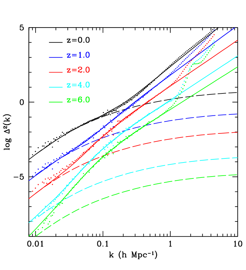
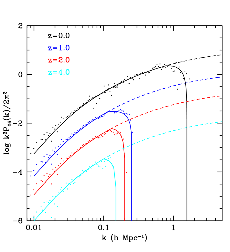
Our measurements of the $\mathcal{P}_{\dot{\Phi}\dot{\Phi}}(k,z)$ power spectrum are shown in Fig. 1. The results from linear theory are also plotted. We find the total scaled $\dot{\Phi}$ power spectrum can be well fitted by a broken power law plus the linear scaled $\dot{\Phi}$ power spectrum $\mathcal{P}_{\dot{\Phi}\dot{\Phi}}=\mathcal{P}_{\dot{\Phi}\dot{\Phi}}^{\rm{nonlin}}+\mathcal{P}_{\dot{\Phi}\dot{\Phi}}^{\rm{lin}}$, where

$$\mathcal{P}_{\dot{\Phi}\dot{\Phi}}^{\rm{nonlin}}(k,z)=\frac{A}{(10k)^{-4/0.75}+(10k)^{-4/B}}.$$ (8)

Here A and B are two free parameters that we use to fit the model to the simulation results at each redshift up to $z=6$. To interpolate the model to intermediate redshifts we linearly interpolate the values of A and B from the nearest two simulation outputs. Our model is compared to the simulation results in Fig. 1.

Figure 3: Evolution of the $\dot{\Phi}$ power spectrum $\Delta^{2}(k)\equiv k^{3}\mathcal{P}_{\dot{\Phi}\dot{\Phi}}(k)/2\pi^{2}$ for specific spatial (left) and angular (right) modes. The solid lines show our model of the simulation results. The dashed lines show the results of linear theory. The power $\Delta^{2}(k)$ decreases monotonically as a function of $z$ at all scales in linear theory. However, the total power seems to be independent of $z$ at high redshift. The deviation from linear theory increases with $z$ and $k$. The angular power spectrum $\Delta^{2}(l)$ shows no deviation from linear theory up to $l=10$. For $l>50$, deviations appear at all redshifts.

We see in Fig. 1 that the linear theory reproduces the ISW+RS $\mathcal{P}_{\dot{\Phi}\dot{\Phi}}$ at $z=0$ only at $k<0.1$ $h$ Mpc^-1. It fails at progressively larger scales as the redshift increases. By $z=2$, linear theory agrees with the simulation results only at $k<0.02$ $h$ Mpc^-1. The reason for this surprising behaviour is that the linear part of the $\mathcal{P}_{\dot{\Phi}\dot{\Phi}}$ drops quickly to zero as the relative importance of $\Omega_{\Lambda}$ diminishes at high redshift, while the non-linear part evolves more slowly with redshift. Therefore, the deviation of the total power spectrum from linear theory happens at larger scales at higher redshifts. We find that the momentum power spectrum, $P_{\dot{\delta}\dot{\delta}}$, and the correlation power spectrum of the density and momentum, $P_{\delta\dot{\delta}}$, behave similarly to the $P_{\dot{\Phi}\dot{\Phi}}$ power spectrum, namely, their deviation from linear theory occurs at larger scales at higher redshift. This is in contrast with the power spectrum of the density field which deviates from linear theory on progressively larger scales at lower and lower redshift. In another words, at the same redshift, the deviation from linear theory occurs at smaller scales for the density field than for the other fields.

The sharp increase of $\mathcal{P}_{\dot{\Phi}\dot{\Phi}}$ measured from the simulation at small scales ($k>1$ $h$ Mpc^-1) is due to discreteness in the $448^{3}$ particle L-BASICC simulation. We used the much higher resolution $2160^{3}$ particle Millennium simulation (Springel et al., 2005) to verify that our model remains accurate at smaller scales and is robust to shot noise corrections.

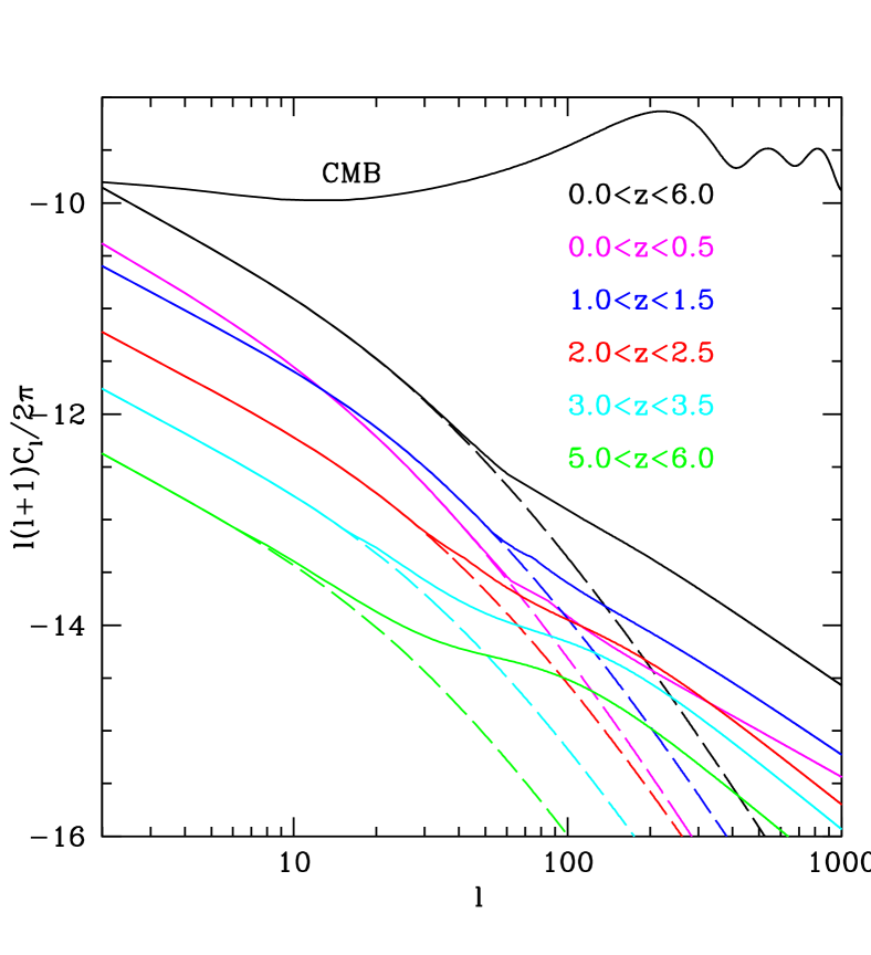
We can now compute the induced angular power spectrum of CMB temperature fluctuations by performing the integral in equation (2) over the redshift range $0<z<6$ using our model for the 3-D power spectrum, $P_{\dot{\Phi}\dot{\Phi}}(k,z)$. The overall result is shown in Fig. 2 along with the contributions coming from different redshift intervals. For the overall angular power spectrum the deviation of the model from the linear theory happens at $l\sim$100. This result confirms the prediction of Cooray (2002b) based on the halo model. However, we also see that the failure of linear theory, as judged by our simulation results, occurs at smaller and smaller $l$ as redshift increases. For example, above $z=5$, the deviation occurs at $l<20$ and, for larger values of $l$ than this, linear theory becomes extremely inaccurate.

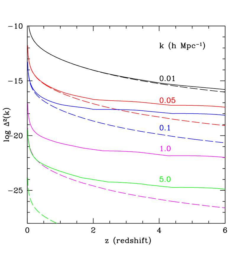
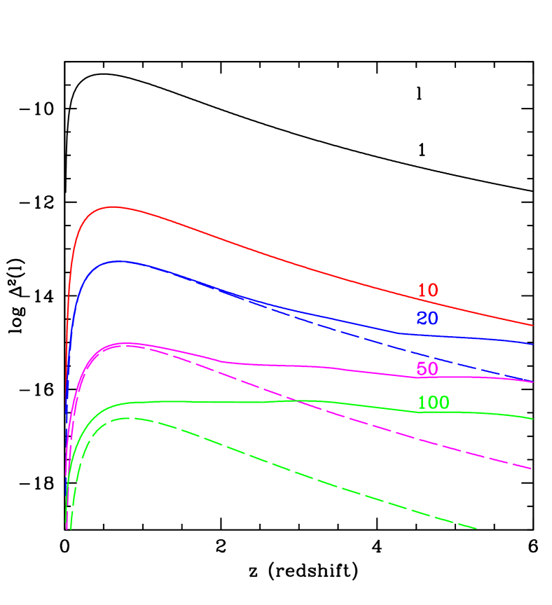
In order to evaluate how the breakdown of linear theory depends on redshift, we plot the evolution of the $\dot{\Phi}$ power at a given scale as a function of redshift in Fig. 3. Generally, the deviations of linear theory from the simulation results decrease with scale and increase with redshift. At $k=0.01$ $h$ Mpc^-1, deviations start to be seen at $z\sim 3$ and, at $k=0.1$ $h$ Mpc^-1, linear theory has become inaccurate at all redshifts. In the right-hand panel, which shows results in $l$ space, we find no deviations up to $l\sim 10$, but for $l>50$, linear theory has clearly broken down at all redshifts. Interestingly, at high redshift, the $\dot{\Phi}$ power in the simulation appears to be independent of $z$ while, in linear theory, this quantity drops monotonically with $z$.

3 the LSS-CMB cross-correlation

Figure 4: $Left$: The cross power spectrum of $\dot{\Phi}$ with $\delta$ at different redshifts. The dotted lines represent the measurements from the L-BASICC and the dashed lines linear theory. The solid lines are our model fit to the sum of the linear theory and the non-linear contribution in the L-BASICC simulation. The non-linear effect begins to appear at $k\sim 1$ $h$ Mpc^-1 at $z=0$, and at larger scales at higher redshifts. It rapidly suppresses the cross power spectrum and causes it to become negative on small scales. $Right$: the same as the left panel but on a linear scale.

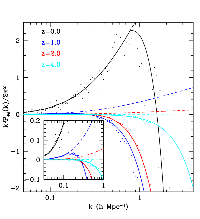
To illustrate the contribution of the Rees-Sciama effect to the cross-correlation of the density field $\delta$ with $\dot{\Phi}$, we can compute the 3-D cross-correlation power spectrum $P_{\dot{\Phi}\delta}(k,z)=<\dot{\Phi}(\vec{k},z)\delta^{*}(\vec{k},z)>$ from our simulations:

$$\mathcal{P}_{\dot{\Phi}\delta}(k,z)=P_{\delta\delta}(k,z)-\frac{P_{\dot{\delta}\delta}(k,z)}{H(z)}$$ (9)

In linear theory, $\mathcal{P}_{\dot{\Phi}\delta}(k,z)=D^{2}(1-\beta)P_{\delta\delta}^{\rm{lin}}(k)$, where $P_{\delta\delta}^{\rm{lin}}(k)$ is the linear density power spectrum at the present time. Results from our simulations are shown in Fig. 4. Comparing with linear theory, we find that the non-linear contribution appears at somewhat smaller scales than that of the autocorrelation power spectrum of $\dot{\Phi}$. At $z=0$, the deviation occurs at $k\sim 1$ $h$ Mpc^-1. However, it then dominates rapidly, making the cross-correlation power spectrum negative. This indicates that once the non-linear effect dominates, the potential of overdense regions evolves faster than the expansion of the universe, becoming deeper and thus imparting a net redshift to CMB photons passing through them. The sense of the effect from underdense regions is reversed, but the effect generated by the overdense regions is dominant and induces a negative cross-correlation between the CMB and the LSS.

To quantify the effect on the large-scale ISW cross-correlation measurements, we model the 3-D cross power spectrum from the simulations at each redshift output. We use linear theory to model the linear regime but once the cross power spectrum starts to deviate from linear theory, we fit it with a function of the form $k^{3}P_{\dot{\Phi}\delta}(k)=A_{1}+A_{2}k+A_{3}k^{2}$, where $A_{1},A_{2}$ and $A_{3}$ are free parameters. Interpolating to intermediate redshifts, we are then able to calculate the projected 2-D power spectrum.

The cross-correlation between LSS and CMB maps has been shown to be a powerful tool for verifying the existence of dark energy and constraining its properties. Current measurements of the cross-correlation have low statistical significance because the volumes probed by LSS surveys are relatively small, but this situation will improve greatly with upcoming surveys. For example, Pan-STARRS1 will survey three quarters of the sky, obtaining photometry for galaxies up to $\sim 24.6$ mag in the $g$-band. The mean galaxy redshift in this “$3\pi$ survey” will be $\bar{z}\sim 0.5$. Pan-STARRS1 will also carry out a deeper but smaller “MDS” survey covering 84 sq deg of the sky to $\sim 27.3$ mag in $g$ for which $\bar{z}\sim 0.8$ (Cai et al., 2008). Cross-correlating such photometric redshift galaxy samples with a CMB map (from WMAP or Planck) will make it possible for the first time to perform ISW tomography. Galaxy samples would be divided into different redshift slices and each one cross-correlated with the CMB map. Values of the dark energy equation of state parameter, $w$, could then be measured using the results from the different redshift slices, effectively constraining the evolution of $w$.

To illustrate how ISW tomography may work, we follow Baugh & Efstathiou (1993) and model the redshift distribution of galaxies tracing the LSS as

$$N(z)\propto\begin{cases}(z-z_{c})^{2}\exp\left[-(\frac{z-z_{c}}{z_{0}})^{3/2}\right]&\text{if $z\leq z_{c}$}\\ 0&\text{if $z>z_{c}$},\end{cases}$$ (10)

but then choose the parameters $z_{0}$ and $z_{c}$ to emulate plausible photometric redshift slices. (The same functional form was also taken by Cabré et al. (2006) to model the SDSS LRG sample.) We assume $z_{0}=0.2$ so that the width of $N(z)$ is much greater than the expected photometric redshift errors. We shift the function into different redshift intervals by using $z_{c}=0,1,2$ and $3$. The median redshift of these samples is $\bar{z}\approx 1.4z_{0}+z_{c}=0.28,1.28,2.28$ and $3.28$ respectively. The cross-correlation power spectrum (derived in an analogous way to the auto-correlation function detailed in the appendix) is given as:

$$C_{l}^{\dot{\Phi}-g}\approx\frac{2}{c^{2}}\int_{0}^{z_{L}}P_{\dot{\Phi}\delta}(k=\frac{l}{r},z)b(z)N(z)H(z)/r^{2}dz,$$ (11)

where $P_{\dot{\Phi}\delta}(k,z)$ is the cross power spectrum of the potential field and the galaxy density field, $b(z)$ is the galaxy bias parameter at redshift $z$, and $N(z)$ is the normalised galaxy selection function, where $\int N(z)dz=1$. We adopt the small angle approximation in which $k=l/r(z)$, where $r(z)$ is the comoving distance. For simplicity, in this illustration, we assume the galaxy bias parameter to be unity. In angular space, the cross-correlation becomes:

$$w^{\dot{\Phi}-g}(\theta)=\sum_{l}\frac{2l+1}{4\pi}P_{l}(\cos\theta)C^{\dot{\Phi}-g}_{l},$$ (12)

where $P_{l}$ are Legendre polynomials. In actual measurements of CMB fluctuations, the monopole and dipole are subtracted. Therefore, we set the power at $l=0$ and $l=1$ to zero before converting the signal into real space. To ensure that the results at smaller angles ($\theta<1^{\circ}$) converge accurately, we sum the power up to $l=10\,000$.

Figure 5: $Left$: The cross-correlation power spectrum of galaxy samples at different $\bar{z}$ with the CMB. The dashed lines are given by linear theory. The solid lines are the sum of the linear theory and the non-linear contribution, which is given by our model fitted to the L-BASICC simulation. The non-linear effect begins to appear at $l\sim 500$. It rapidly makes the cross power spectrum become negative. $Right$: The cross-correlation of galaxy samples at different $\bar{z}$ with the CMB in angular space. The non-linear effect suppresses the ISW effect at sub-degree scales. It is negligible at low redshifts and large scales.

The cross-correlation results are shown in Fig. 5. The contribution from the non-linear RS effect can be seen to become increasingly important as the redshift of the sample increases. The cross-correlation power spectrum decreases and deviates from linear theory rapidly at $l\sim 500$ due to the non-linear effect. It turns negative at $l\sim 1000$. This result is consistent with that obtained by Nishizawa et al. (2008) who used a similar method to illustrate the impact of the ISW and RS effects on the CMB-weak lensing cross-correlation. In angular coordinates, shown on the right-hand panel, the RS effect is negligible at $\theta>1^{\circ}$ at all redshifts. For the high redshift samples, it becomes important at sub-degree scales for the high redshift samples where it suppresses the cross-correlation power spectrum by about $5-10\%$ at acrminute scales.

The statistical significance of current measurements of the CMB-LSS cross-correlation is not yet high enough to detect the effects we are discussing. Most current measurements can only determine the cross-correlation at degree scales or above (e.g. Cabré et al., 2006). Future CMB or SZ surveys with high resolution might be able to resolve this contribution.

4 Conclusions

We have used an N-body simulation to calculate the non-linear (Rees-Sciama) contribution to the Integrated Sachs Wolfe effect. The comparison of the 3-D and 2-D power spectra measured from the simulation with those given by linear theory reveals a strong nonlinear contribution whose physical scale increase with redshift. We investigated the strength of this effect on the cross-correlation of the CMB with galaxy samples in terms of angular power spectra and in angular coordinates at different redshifts. We find that there is a non-linear contribution to the cross-correlation signal at sub-degree scales. The non-linear effect alters not only the amplitude, but also the shape of the cross-correlation power spectrum. With current galaxy samples which cover relatively small volumes, it is not yet possible to disentangle the contribution of the RS effect from that of the ISW effect within the noise. However, in future surveys like Pan-STARRS and LSST, for which the number of galaxies and the sky coverage will increase dramatically, the error bars on the cross-correlation will be much smaller. In this case, the importance of the Rees-Sciama effect may become significant for high redshift samples. The effect of the non-linear cross-correlation at scales of arcminutes would contaminate the SZ signal in the CMB and this could confuse its interpretation (e.g. Fosalba et al., 2003; Diego et al., 2003; Myers et al., 2004; Lieu et al., 2006; Cao et al., 2006; Bielby & Shanks, 2007).

Our analysis is based on a simulation that assumes a $\Lambda$CDM cosmology. The non-linear contribution depends on the values of the cosmological parameters. In a flat universe with a cosmological constant, the RS effect will become increasingly dominant relative to the ISW effect as the value of $\Omega_{\Lambda}$ decreases. In the most extreme case, if $\Omega_{\Lambda}=0.0$, the ISW effect will vanish, leaving only the RS effect (Seljak, 1996). The analysis of this paper could be generalized either using re-normalised perturbation theory (e.g. Crocce & Scoccimarro, 2006), or simulations with different dark energy models. In any case, more general modelling of the non-linear effect will be required for an accurate interpretation of future measurements of the LSS-CMB cross-correlation.

Appendix A Angular Power Spectra

Here we derive the relationship between the 3-D power spectrum of gravitational potential fluctuations, $P_{\dot{\Phi}\dot{\Phi}}(k,t)=(2\pi)^{-3}\langle\dot{\Phi}(k,t)\dot{\Phi}^{*}(k,t)\rangle$ and the resulting angular power spectrum of the induced CMB temperature fluctuations. Expanding the pattern of temperature fluctuations, $\Delta T(\hat{r})/{\bar{T}_{0}}$, in terms of spherical harmonics we have

$$a_{lm}=\int\frac{\Delta T(\hat{r})}{\bar{T}_{0}}\ Y_{lm}^{*}(\hat{r})\,d\hat{r}$$ (13)

which using equation (1) becomes

$$a_{lm}=-\frac{2}{c^{2}}\int Y_{lm}^{*}(\hat{r})\int_{0}^{t_{L}}\dot{\Phi}(\hat{r},t)\,dt\,d\hat{r}.$$ (14)

Writing $\dot{\Phi}(\hat{r},t)$ in terms of a Fourier expansion and using the spherical harmonic expansion of a plane wave, $\exp(i\vec{k}\cdot\vec{r})=4\pi\sum_{lm}i^{l}j_{l}(kr)Y_{lm}^{*}(\hat{k})Y_{lm}(\hat{r})$ this becomes

$$a_{lm} =-\frac{2}{(2\pi)^{3}c^{2}}\int Y_{lm}^{*}(\hat{r})\int_{0}^{t_{L}}\int\dot{\Phi}(\vec{k},t)\exp(i\vec{k}\cdot\vec{r})d\vec{k}dtd\hat{r}$$ (15)

$$=-\frac{2\times 4\pi}{(2\pi)^{3}c^{2}}\int Y_{lm}^{*}(\hat{r})\int_{0}^{t_{L}}\int\dot{\Phi}(\vec{k},t)\times$$

$$\quad\sum_{l^{\prime}m^{\prime}}i^{l}j_{l}(kr)Y_{l^{\prime}m^{\prime}}^{*}(\hat{k})Y_{l^{\prime}m^{\prime}}(\hat{r})\,d\vec{k}\,dt\,d\hat{r}$$

$$=-\frac{1}{\pi^{2}c^{2}}\int_{0}^{t_{L}}\int\dot{\Phi}(\vec{k},t)i^{l}j_{l}(kr)Y_{lm}^{*}(\hat{k})\,d\vec{k}\,dt.$$

Hence the angular power spectrum, $C_{l}$, is given by

$$C_{l}\,\delta_{ll^{\prime}}\delta_{mm^{\prime}}\equiv\left\langle a_{lm}a_{l^{\prime}m^{\prime}}^{*}\right\rangle$$ (16)

$$=\left[\frac{1}{\pi^{2}c^{2}}\right]^{2}\Big{\langle}\int_{0}^{r_{L}}\int\dot{\Phi}(\vec{k},r)i^{l}j_{l}(kr)Y_{lm}^{*}(\hat{k})\,d\vec{k}\,dr$$

$$\quad\times\int_{0}^{r_{L}}\int\dot{\Phi}^{*}(\vec{k}^{\prime},r^{\prime})i^{l^{\prime}}j_{l}(k^{\prime}r^{\prime})Y_{l^{\prime}m^{\prime}}(\hat{k}^{\prime})d\vec{k}^{\prime}dr^{\prime}\Big{\rangle}.$$

Using the identity $\left\langle\dot{\Phi}(\vec{k})\dot{\Phi}^{*}(\vec{k}^{\prime})\right\rangle\equiv(2\pi)^{3}\delta(\vec{k}-\vec{k}^{\prime})P_{\dot{\Phi}\dot{\Phi}}(k)$ and the orthogonality relationship of spherical harmonics

$$\int_{4\pi}Y_{lm}^{*}(\hat{r})Y_{l^{\prime}m^{\prime}}(\hat{r})\,d\hat{r}=\delta_{ll^{\prime}}\delta_{mm^{\prime}}$$ (17)

this becomes

$$C_{l}\,\delta_{ll^{\prime}}\delta_{mm^{\prime}}=\frac{8}{\pi c^{4}}\frac{2}{\pi}\int\int_{0}^{r_{L}}\int_{0}^{r_{L}}P_{\dot{\Phi}\dot{\Phi}}(k,r,r^{\prime})i^{l}j_{l}(kr)Y_{lm}^{*}(\hat{k})$$ (18)

$$\quad\times i^{l^{\prime}}j_{l}(kr^{\prime})Y_{l^{\prime}m^{\prime}}(\hat{k})\,dr^{\prime}\,dr\,d\vec{k}$$

$$=\frac{8}{\pi c^{4}}\int\int_{0}^{r_{L}}\int_{0}^{r_{L}}k^{2}P_{\dot{\Phi}\dot{\Phi}}(k,r,r^{\prime})j_{l}(kr)j_{l}(kr^{\prime})dr^{\prime}drdk\delta_{ll^{\prime}}\delta_{mm^{\prime}}$$

$$C_{l}=\frac{8}{\pi c^{4}}\int\int_{0}^{r_{L}}\int_{0}^{r_{L}}k^{2}P_{\dot{\Phi}\dot{\Phi}}(k,r,r^{\prime})j_{l}(kr)j_{l}(kr^{\prime})dr^{\prime}drdk.$$

This exact relationship can be simplified by using Limber’s approximation. For small angular separations, $\theta$, at comoving distance, $r$, the wave number, $k$, can be expressed in terms of its components parallel and perpendicular to the line of sight and approximated by $k=\sqrt{k_{\parallel}^{2}+k_{\perp}^{2}}\approx k_{\perp}$, where $k_{\perp}=2\pi/r\theta\approx l/r\gg k_{\parallel}\sim 1/\Delta r$, namely, the power is dominated by that perpendicular to the line of sight and there is no correlation between different shells of $\Delta r$ along the line of sight. Combining this with the orthogonality relation for spherical Bessel functions,

$${2\over\pi}\int k^{2}j_{l}(kr)j_{l}(kr^{\prime})dk=\delta(r-r^{\prime})/r^{2},$$ (19)

we arrive at

$$C_{l}\approx\frac{4}{c^{4}}\int_{0}^{r_{L}}P_{\dot{\Phi}\dot{\Phi}}(k=\frac{l}{r},r)/r^{2}dr.$$ (20)

(see also Limber, 1954; Kaiser, 1992; Hu, 2000; Verde et al., 2000). Verde et al. (2000) find that the difference between this approximation and the full calculation is less than $3\%$ at $l>20$. In this paper we are mainly concerned with even smaller scales ($l>500$) and so we are justified in using Limber’s approximation. We also tested the difference between using $k=l/r$ and the more accurate $k=(l+1/2)/r$ (Loverde & Afshordi, 2008) and find very little difference to our results.

References

- Afshordi et al. (2004) Afshordi N., Loh Y.-S., Strauss M. A., 2004, Phys. Rev. D, 69, 083524
- Angulo et al. (2008) Angulo R. E., Baugh C. M., Frenk C. S., et al. 2008, MNRAS, 383, 755
- Baugh & Efstathiou (1993) Baugh C. M., Efstathiou G., 1993, MNRAS, 265, 145
- Bielby & Shanks (2007) Bielby R. M., Shanks T., 2007, MNRAS, 382, 1196
- Cabré et al. (2006) Cabré A., Gaztañaga E., Manera M., et al. 2006, MNRAS, 372, L23
- Cai et al. (2008) Cai Y., Angulo R. E., Baugh C. M., et al. 2008, arXiv:0810.2300
- Cao et al. (2006) Cao L., Chu Y.-Q., Fang L.-Z., 2006, MNRAS, 369, 645
- Cooray (2002a) Cooray A., 2002a, Phys. Rev. D, 65, 103510
- Cooray (2002b) Cooray A., 2002b, Phys. Rev. D, 65, 083518
- Crocce & Scoccimarro (2006) Crocce M., Scoccimarro R., 2006, Phys. Rev. D, 73, 063519
- Diego et al. (2003) Diego J. M., Silk J., Sliwa W., 2003, MNRAS, 346, 940
- Efstathiou et al. (2002) Efstathiou G., Moody S., Peacock J. A., et al. 2002, MNRAS, 330, L29
- Fan & Chiueh (2001) Fan Z., Chiueh T., 2001, ApJ, 550, 547
- Fosalba & Gaztañaga (2004) Fosalba P., Gaztañaga E., 2004, MNRAS, 350, L37
- Fosalba et al. (2003) Fosalba P., Gaztañaga E., Castander F. J., 2003, ApJ, 597, L89
- Giannantonio & Crittenden (2007) Giannantonio T., Crittenden R., 2007, MNRAS, 381, 819
- Granett et al. (2008) Granett B. R., Neyrinck M. C., Szapudi I., 2008, ArXiv e-prints, 805
- Hinshaw et al. (2008) Hinshaw G., Weiland J. L., Hill R. S., et al. 2008, ArXiv e-prints, 803
- Hu (2000) Hu W., 2000, ApJ, 529, 12
- Kaiser (1992) Kaiser N., 1992, ApJ, 388, 272
- Lieu et al. (2006) Lieu R., Mittaz J. P. D., Zhang S.-N., 2006, ApJ, 648, 176
- Limber (1954) Limber D. N., 1954, ApJ, 119, 655
- Loverde & Afshordi (2008) Loverde M., Afshordi N., 2008, Phys. Rev. D, 78, 123506
- Loverde et al. (2007) Loverde M., Hui L., Gaztañaga E., 2007, Phys. Rev. D, 75, 043519
- McEwen et al. (2007) McEwen J. D., Vielva P., Hobson M. P., et al. 2007, MNRAS, 376, 1211
- Mei & Bartlett (2004) Mei S., Bartlett J. G., 2004, A&A, 425, 1
- Myers et al. (2004) Myers A. D., Shanks T., Outram P. J., Frith W. J., Wolfendale A. W., 2004, MNRAS, 347, L67
- Nishizawa et al. (2008) Nishizawa A. J., Komatsu E., Yoshida N., Takahashi R., Sugiyama N., 2008, ApJ, 676, L93
- Padmanabhan et al. (2005) Padmanabhan N., Hirata C. M., Seljak U., et al. 2005, Phys. Rev. D, 72, 043525
- Perlmutter et al. (1999) Perlmutter S., Aldering G., Goldhaber G., et al. 1999, ApJ, 517, 565
- Puchades et al. (2006) Puchades N., Fullana M. J., Arnau J. V., Sáez D., 2006, MNRAS, 370, 1849
- Raccanelli et al. (2008) Raccanelli A., Bonaldi A., Negrello M., et al. 2008, ArXiv e-prints, 802
- Rassat et al. (2007) Rassat A., Land K., Lahav O., et al. 2007, MNRAS, 377, 1085
- Rees & Sciama (1968) Rees M. J., Sciama D. W., 1968, Nature, 217, 511
- Riess et al. (1998) Riess A. G., Filippenko A. V., Challis P., et al. 1998, AJ, 116, 1009
- Sachs & Wolfe (1967) Sachs R. K., Wolfe A. M., 1967, ApJ, 147, 73
- Seljak (1996) Seljak U., 1996, ApJ, 460, 549
- Smith et al. (2003) Smith R. E., Peacock J. A., Jenkins A., White S. D. M., Frenk C. S., Pearce F. R., Thomas P. A., Efstathiou G., Couchman H. M. P., 2003, MNRAS, 341, 1311
- Spergel et al. (2003) Spergel D. N., Verde L., Peiris H. V., et al. 2003, ApJS, 148, 175
- Springel et al. (2005) Springel V., White S. D. M., Jenkins A., et al. 2005, Nature, 435, 629
- Sunyaev & Zeldovich (1972) Sunyaev R. A., Zeldovich Y. B., 1972, Comments on Astrophysics and Space Physics, 4, 173
- Verde et al. (2000) Verde L., Heavens A. F., Matarrese S., 2000, MNRAS, 318, 584
- White et al. (1993) White S. D. M., Efstathiou G., Frenk C. S., 1993, MNRAS, 262, 1023