Spatial features of population dynamics arising from
mutual interaction of different age groups in rodents

Abstract

We study the dynamics of the transmission of the hanta virus infection among mouse populations, taking into account, simultaneously, seasonal variations of the environment and interactions within two classes in the mouse population: adults and subadults. The interactions considered are not symmetric between the two age-organized classes and are responsible for driving the younger members away from home ranges. We consider the case of a bounded habitat affected by seasonal variations.  

I Introduction

Theoretical investigations of population dynamics of animals such as mice or other rodents derive their current importance both from their direct relevance to the spread of epidemics such as the Hantavirus YATES ; AK ; PASI ; KPHA ; KLAC but also from the interplay of the approaches of physics and ecology that such investigations encourage MURR ; LI ; COSNER ; Levin ; KOT . Our interest in the present paper is on prevalent effects of the competitive interaction among adults and subadults among rodent populations. Several ecological studies have shown the importance of such an interaction fgt1 ; fgt2 . The interaction can be studied by considering an age-structured population of mice, i.e., by splitting the population into classes organized by age. There is competitive struggle for territory associated with the fact that the occurrence of infected cases of several types of Hantavirus is mostly observed among adult individuals. This, in turn, is related to the proposed mechanism of infection among rodents: territorial fights that produce wounds on the animals as a tangible and verifiable consequence. The subadult population, consisting of smaller-sized individuals, tends to maintain its distance from the fights, and is thus less susceptible to infection. The effect of remaining not too close to the source of the fights, viz., the adult population, subadult individuals are forced to abandon the already colonized spaces and are therefore driven to new habitats, most of the time less suitable for survival.

We propose here a model considering an age-structured population composed by the two well differentiated groups we have mentioned above: subadults and adults. A third group, composed by juvenile individuals may be taken into account but will be left out of our calculations as relatively unimportant.

Like previous models AK ; PASI ; KPHA ; KLAC , ours is based on a set of Fisher-like equations FISHER to describe the evolution of the population of individuals of each group whose densities we will respectively denote by $M_{a}$ and $M_{y}$. Here, the suffix $a$ stands for adults and the suffix $y$ for the young individuals, the subadults.

II The model

The specific set of equations in our model would be, in the absence of territorial interactions,

$$\frac{\partial M_{a}}{\partial t} = D_{a}\nabla^{2}M_{a}+\mu M_{y}-\delta M_{a}-\frac{M_{a}M}{K(t)},$$

$$\frac{\partial M_{y}}{\partial t} = D_{y}\nabla^{2}M_{y}+\beta M_{a}-\mu M_{y}-\frac{M_{y}M}{K(t)}.$$

Here we are considering different diffusion coefficients $D_{a}$ and $D_{y}$ for the adults and the subadults, to take into account the fact that adult individuals tend to remain in a rather bounded area, considered as each individual territory, while the subadults tend to move further and probably faster. One would therefore expect $D_{a}<D_{y}.$ The term in each of the above equations which is associated with the competition for resources, is characterized by what is called the environmental parameter $K$ and is proportional to the so-called carrying capacity. We will take $K$ to be time dependent because of seasonal variations. We denote the total population of the mice by $M=M_{a}+M_{y}$. The rate $\mu$ is one of transformation of subadults into adults through the process of maturity, thus is proportional to the subadult population and appears with reversed sign in the two equations. The subadults are born from the adults at $\beta$, the birth rate. Death of the adults occurs at rate $\delta$ and we have omitted it from the subadult population equation for simplicity and to reflect the simplifying assumption that natural death visits only the adults. If predators were introduced into our considerations different rates might be put into the equations including a death rate for the subadults.

In this work we propose to modify the above set of equations to take into account the ecologically important experimental observation related to territorial fights. Due to competition for the conquest and preservation of the home range, adult mice tend to fight among themselves. Indeed, these fights have been suspected to constitute one of the most important ways of transmission of the Hantavirus among rodents of the same species. As a result of these territorial threats of the adults, the subadults, being smaller in size, are forced to abandon already colonized environments and move towards unoccupied spaces. There are at least two different ways to include this tendency into the equation. To take into account the fact that subadults will tend to move away from places with high adult occupation, we may assume the subadult flux to be proportional to the gradient of the adult population, $\nabla M_{a}$; at the same time, no subadult flux is possible in the absence of young individuals. Thus, the interaction term should be proportional to the population of the subadults $M_{y}$ as well as to the adult gradient. The resulting set of equations is

$$\frac{dM_{a}}{dt} = D_{a}\nabla^{2}M_{a}+\mu M_{y}-\delta M_{a}-\frac{M_{a}M}{K(t)}$$

$$\frac{dM_{y}}{dt} = D_{y}\nabla^{2}M_{y}+\beta M_{a}-\mu M_{y}-\frac{M_{y}M}{K(t)}$$

$$+\kappa\nabla(M_{y}\nabla M_{a})$$

with $\kappa$ a constant that determines the strength of the interaction.

The other manner that young individuals might tend to get away from populated areas is by creating a flux of their own class which is proportional to the local density of the other class, i.e., the adult. Under these conditions we will have

$$\frac{dM_{a}}{dt} = D_{a}\nabla^{2}M_{a}+\mu M_{y}-\delta M_{a}-\frac{M_{a}M}{K(t)}$$

$$\frac{dM_{y}}{dt} = D_{y}\nabla^{2}M_{y}+\beta M_{a}-\mu M_{y}-\frac{M_{y}M}{K(t)}$$

$$+\kappa\nabla(M_{a}\nabla M_{y}).$$

Comparison of the two new interaction expressions,

$$\nabla(M_{y}\nabla M_{a})=(\nabla M_{a})(\nabla M_{y})+M_{y}\nabla^{2}M_{a}$$

and

$$\nabla(M_{a}\nabla M_{y})=(\nabla M_{a})(\nabla M_{y})+M_{a}\nabla^{2}M_{y}$$

shows that they share a common term proportional to the gradient of each of the classes and another term which in one case is proportional to the density of subadult population and the Laplacian of the adult population and in the other case the situation is precisely reversed.

In both cases there is a homogeneous nontrivial non-negative steady state solution, for Eqs. (LABEL:fish), (LABEL:chem1) or (LABEL:chem2) that can be written in terms of the parameters of the problem $\beta$, $\delta$, $\mu$ and $K$, and is independent of the interaction strength $\kappa$:

$$M_{a}^{0} = \frac{K}{2(\beta-\delta)}(\delta(\delta+A)+\mu(2\beta-\mu+A))$$

$$M_{y}^{0} = \frac{K}{2(\beta-\delta)}[(\mu(\delta-\mu+{A})$$ (4)

$$-\beta(\delta+3\mu-{A}))]$$

where $A=\sqrt{\delta^{2}+4\beta\mu-2\,\delta\mu+\mu^{2}}.$ In the following section we will study Eqs.(LABEL:chem1)and (LABEL:chem2), i.e. we will analyze the effects of each of the new terms separately.

We are interested in effects of temporal or seasonal changes in the environment. These changes will be reflected in a change in the carrying capacity of the habitat. Therefore, we will consider a varying $K$. The ability of a given species to adapt to a changing environment is related to their mobility as well as to other quantities such as the birth and death rates. One way to characterize the mobility is by considering the so-called Fisher velocity of the species associated with traveling environments which can naturally arise as the seasons change. When favorable conditions move in space and time, it is important to find out how the population can or cannot follow them, and whether there are critical velocities of the traveling environment which separate parameters regions in which the species survive or undergo extinction. To facilitate the subsequent discussion we introduce the concept of a refugium, a bounded domain with a high carrying capacity. The population of a given species can live within this region. Outside the refugium, the living conditions are too harsh for the species to survive.

III Static refugium

When no temporal variations of the refugium are considered, we find stationary profiles for both populations which differ from those previously found when considering Fisher-like coupled equations. In Figs.1 we display the profiles of both populations in three cases. All parameters of the problem are the same in all cases, with the exception of $\kappa$ which is $0$ in (a) but, in arbitrary units, $10$ in (b) and (c).

We can see that while the profile of the adult density $M_{a}$ remains almost unchanged in the presence of interactions, that of the subadult density $M_{y}$ presents interesting effects. Since the interactions tend to drive the subadults away from the adults, in both cases there is an increase of the number of individuals at the borders of the refugium. The effect of the interaction term is more evident in regions where the gradient of $M_{a}$ is greater. This fact explains the shoulder on the profile of $M_{y}$ in Fig. 1.b. On the other side, the profile in Fig. 1.c presents the smoothest shape, consistent with a greater effective diffusion coefficient.

Figure 1: Steady state profiles of $M_{a}$ (solid)and $M_{y}$ (dashed)in a bounded domain. The plots correspond to the solution to (a) Eqs.(LABEL:fish), (b) Eqs.(LABEL:chem1), (c) Eqs.(LABEL:chem2). Case (a) represents no interaction whereas cases (b) and (c) describe the two different interactions considered (see text). Parameters (arbitrary units) are $\beta=4$, $\mu=0.4$, $\delta=0$, $\kappa=10$. Additionally the environment parameter $K$ is $10^{-4}$ (practically zero) outside and 9 inside the refugium.

The interaction term affects not only the shape of the profile of both population but also the maximum values attained by the population inside the refugium. We note that the solutions in Eq.(4), where $\kappa$ plays no role, correspond to infinite domains. When bounded domains are considered, $D_{a}$, $D_{y}$, as well as $\kappa$ and the domain size, affect the maximum value of the population. We plotted In Fig. 2 the behavior of the maximum attained by $M_{y}$, $M_{y}^{max}$, for a given size of the refugium and constant diffusion coefficients as a function of the values of $\kappa$.

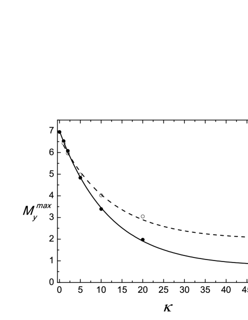
Figure 2: Maximum value of the subadult mouse population $M_{y}$ as a function of the strength $\kappa$ of the interaction between subadults and adults from Eqs. (2) (full circle, solid line ) and Eqs. (3) (empty circle, dashed line). The curves are the result of exponential fitting of the solutions obtained numerically.

The population of subadults undergoes an overall decay as $\kappa$ increases. The curves in Fig. (2) were fitted with decaying exponentials. A mono-exponential fit works in each case.

An interesting effect is the possibility of maintaining a subadult population localized when it is bounded by a population of adults as if they were forming a well confining the younger mice. As the interaction terms prevent the population of subadults from moving towards an increasing gradient of adults, the subadult population remains localized until the population of adults has decreased sufficiently (by diffusion) to reach a state in which diffusion and interaction in the subadult population can compete and delocalize the nucleus of subadults.

IV traveling refugium

Consider now a traveling refugium of constant size. This will allow us to test the ability of the population to survive while following the moving environment. We will find the critical velocity of the refugium $v_{c}$, above which survival is no longer possible. Fig. 3 displays the changes in the fronts as the refugium starts to move in each of the three cases.

Again, while the profile of $M_{a}$ (adults) remains almost unchanged, the profile of $M_{y}$ (subadults) shows some effects. Both interactions (expressed in Eqs. LABEL:chem1 and LABEL:chem2 tend to maintain the symmetry of the distribution of the population despite the translational movement; the effect of Eqs. LABEL:chem2 is with stronger intensity as it strongly biases the population contrary to the movement.

Figure 3: Steady state profiles of $M_{a}$ (solid)and $M_{y}$ (dashed)in a traveling bounded domain with velocity $v=1.3$. The plots correspond to the solution to (a) Eqs.(LABEL:fish), (b) Eqs.(LABEL:chem1), (c) Eqs.(LABEL:chem2). With $\beta=4$, $\mu=0.4$, $\delta=0$, $\kappa=10$ and $K=9$ inside the bubble. Parameters are in arbitrary units.

When considering only one species and the Fisher equation, the critical velocity is given by the Fisher velocity $v_{f}=\sqrt{Da}$, with $D$ the diffusion constant and $a$ the birth rate. When dealing with a set of coupled equations it is still possible to show that there is a critical velocity, associated closely with the critical velocity of the slowest species.

If the new terms in Eqs.(LABEL:chem1) and (LABEL:chem2) are neglected to get Eqs. (LABEL:fish), within the range of the values used for the parameter values of both populations, adult and subadult densities can be shown to be of the same order throughout the whole domain. The adult population would then be described by

$$\frac{dM_{a}}{dt}=D_{a}\nabla^{2}M_{a}+\mu M_{a}-\delta M_{a}-\frac{M_{a}^{2}}{K}.$$ (5)

Figure 4: Critical velocity of the population (relative to the Fisher velocity) as a function of $\kappa$ from Eqs. (2) (full circle, solid line ) and Eqs. (3) (empty circle, dashed line). The curves are exponential fitting of the data.

This would mean that we can associate a Fisher velocity, $v_{f}=\sqrt{D_{a}(\mu-\delta)}$ with the population $M_{a}$. While it appears that a similar argument might be used for $M_{y}$, this is not true because the idea that both populations are of the same order is no longer valid in that case when the velocity of the refugium is above the Fisher velocity for $M_{a}$. The adults are slower than subadults. It is therefore that the lower Fisher velocity appropriately describes the critical situation. This explains the numerical results that show that when considering Eqs(LABEL:fish), the critical velocity of the entire population $v_{c}$ is almost the same as the critical velocity that can be obtained from Eq.(5).

We display in Fig. 4 interaction effects on the critical velocity $v_{c}$ by plotting $v_{c}/v_{f}$ (where $v_{f}$ is the Fisher velocity of the adult mice in the absence of interactions) as a function of the interaction strength $\kappa$ for the two kinds of interaction. We find that the numerical solutions may be fitted excellently by saturating exponentials. We observe that in both cases there is an increase in $v_{c}$ as $\kappa$ increases. The effect is much more evident for Eq.LABEL:chem1 as was expected from the shape presented by its profile in Fig. 3b.

Figure 5: Limiting maximum values $M_{y}^{max+}$(squares) and $M_{y}^{max-}$(circles). Full symbols correspond to Eqs. (2) while empty symbols correspond to Eqs. (3). Curves are exponential fittings of the data

V Breathing refugium

Seasonal variations of the relevant parameters may correspond to the refugium being centered in a static point with its size changing in an oscillating way. We call this case a breathing refugium. To show the new features due to the effect of the interaction terms, we plot the maximum of the subadult density $M_{y}$ as a function of time. If there are no interactions between subadults and adults, the maximum suffers negligible periodic variations. On the other hand, in the presence of interactions, the maximum oscillates between two values displayed in Fig. 5 by squares and circles, respectively. We call these two limiting maximum values $M_{y}^{max+}$ and $M_{y}^{max-}$. The amplitude of this variation increases in a very apparent way as $\kappa$ grows. This is shown in Fig. 6, where we plot the relative difference $\alpha=\frac{M_{y}^{max+}-M_{y}^{max-}}{M_{y}^{max+}}$, which is the ratio of the difference between the limiting maximum values to the greater of these maximum values.

Figure 6: Relative amplitude of the temporal oscillations of the maximum value of $M_{y}(x,t)$ as a function of $\kappa$ from Eqs. (2 )(full circle, solid line ) and Eqs. (3) (empty circle, dashed line). The curves are exponential fitting of the data.

[h]

Figure 7: Comparative intensity of each effect on the border of the moving front of subadult population. The effect associated to Eqs. (LABEL:chem1) is in solid line, while the one corresponding to Eqs. (LABEL:chem2) is in dashed line. The units are arbitrary

VI Conclusions

We have shown the emergence of some interesting effects due to the inclusion of interaction among different groups in a population. We have also compared our new results with those already known from simple Fisher equations with no interactions. Among the new findings are the change in the shape of the steady and traveling profiles (Figs. 1 and 3), the increase of the critical velocity of the populations (Fig. 4) with interaction strength, and the oscillatory behavior of the population profiles when seasonal changes in the environment are considered (Figs. 5 and 6). Some of these results can be understood easily in the context of Fig. 3. When a traveling refugium is considered, the steady fronts displayed in Fig. 1 change. The traveling profile are asymmetric, showing a depletion of the concentration of individuals at the head (right) of the front. In the presence of the interaction, the subadult population tends to move towards areas less populated with adults. This explains the changes in the traveling profiles presented by both population in Figs. 3a and 3b. The effect of the term in Eqs. LABEL:chem1 is stronger than that of the one considered in Eqs.LABEL:chem2. Indeed, we observe that not only the population of subadults moves to the right in a more evident way but the change in the critical velocity is also more intense.

The shape presented by the profiles associated to each of the equations can be understood by qualitative arguments. As mentioned before, a comparison of the two new interaction expressions, shows that they share a common term proportional to the gradient of each of the classes $\nabla(M_{a})(\nabla M_{y})$. The other terms, $M_{y}\nabla^{2}M_{a}$ and $M_{a}\nabla^{2}M_{y}$ respectively, promote a flux of the subadult population towards less populated regions, i. e. to the right of the traveling front. This explains the shift of the profile of subadults. The difference in the resulting profile can be understood when analyzing the difference in intensity of ech term, as shown in Fig. 7, where we compare the intensity of each of the effect when considering a stationary profile. The oscillations found when the refugium is breathing are due to the fact that a system described by any of the Eqs. (LABEL:chem1) or (LABEL:chem2) is much more sensitive to changes in the size of the refugium, as can be observed by the values displayed in Fig. 2, where without loss of generality, only one size of the refugium was analyzed.

This work was supported in part by the NSF under grant no. INT-0336343 and by NSF/NIH Ecology of Infectious Diseases under grant no. EF-0326757.

References

- (1) T. L.Yates, J. N. Mills, C. A. Parmenter, T. G. Ksiazek, R. R. Parmenter, J. R. Vande Castle, C. H. Calisher, S. T. Nichol, K. D. Abbott, J. C. Young, M. L. Morrison, B. J. Beaty, J. L. Dunnum, R. J. Baker, J. Salazar-Bravo, and C. J. Peters. Bioscience 52, 989-998 (2002).
- (2) G. Abramson and V. M. Kenkre, Phys. Rev. E 66, 011912 (2002).
- (3) V. M. Kenkre in Patterns, Noise and Interplay of Nonlinearity and Complexity:Proceedings of the PASI on Modern Challenges in Statistical Mechanics, edited by V. M. Kenkre and K. Lindenberg (AIP New York, 2003).
- (4) V. M. Kenkre, Physica A 356, 121-126 (2005).
- (5) V. M. Kenkre, L. Giuggioli, G. Abramson, and G. Camelo- Neto, Eur. Phys. J. B 55, 461-470, (2007).
- (6) J. D. Murray, Mathematical Biology, 2nd edn, New York, Springer(1993).
- (7) S. P. Petrovskii and Bai-Lian Li, Exactly Solvable Models of Biological Invasion, Chapman & Hall, CRC Press, 2006.
- (8) Robert Cantrell and Chris Cosner, Spatial Ecology via Reaction-Diffusion Equations, Wiley series in Mathematical and Computational Biology, 2003.
- (9) Frontiers in Mathermatical Biology. Lecture Notes in Biomathematics 100, ed. S. A. Levin, (Springer-Verlag, New York 1994).
- (10) M. Kot Elements of Mathematical Ecology (Cambridge University Press, Cambridge, U K, 2003).
- (11) G. E. Glass, J.E. Childs, G.W. Korch, J.W. Le Duc. Epidemiol Infect 101, 459 472 (1988).
- (12) J. J. Root, W. C. Black, C. H. Calisher, K. R. Wilson, B. J. Beaty. Vector-Borne and Zoonotic Diseases, 4, 149-157 (2004).
- (13) R. A. Fisher, Ann. Eugen, London 7, 355-369(1937).
- (14) M. Ballard, V. M. Kenkre, and M. N. Kuperman, Phys. Rev. E 70, 031912 (2004).