Bias dependence of magnetic exchange interactions: application to interlayer exchange coupling in spin valves

Abstract

We study how a bias voltage changes magnetic exchange interactions. We derive a general expression for magnetic exchange interactions for systems coupled to reservoirs under a bias potential, and apply it to spin valves. We find that for metallic systems, the interlayer exchange coupling shows a weak, oscillatory dependence on the bias potential. For tunneling systems, we find a quadratic dependence on the bias potential, and derive an approximate expression for this bias dependence for a toy model. We give general conditions for when the interlayer exchange coupling is a quadratic function of bias potential.

I Introduction

Magnetic multilayers and spin valves exhibit a rich and extremely useful array of magneto-electronic phenomena, including magnetoresistance, interlayer exchange coupling, and spin transfer torque. Spin transfer torque is an effect in which the application of a current can change the relative orientation of the layers’ magnetization. The presence of spin transfer torques are understood as a result of nonequilibrium electron current flow, or more precisely, a spatially varying spin current. Spin currents describe the flow of electron spin, and are tensor objects with two indices: one labeling the direction of flow in real space, the other labeling the vector component of spin. Interlayer exchange coupling is an indirect exchange interaction between magnetic layers, like the Ruderman-Kittel-Kasuya-Yosida (RKKY) interaction, with equilibrium electrons in the nonmagnetic spacer playing the mediating role. Interlayer exchange coupling is closely related to spin transfer torques, as we discuss below. In this paper, we elucidate the relationship between interlayer exchange coupling and spin transfer torques, specifically how the interlayer exchange coupling depends on the applied bias.

Interlayer exchange coupling gives rise to an energetic preference for parallel or anti-parallel alignment of the layers’ magnetization, and is given approximately as $E=-J\hat{M}_{1}\cdot\hat{M}_{2}$, where $\hat{M}_{i}$ are the directions of the magnetizations. It shows RKKY-like characteristics, such as an oscillatory dependence on spacer layer thickness, with a period determined by the spacer material Fermi wave vector. This behavior is well established reviews1 ; reviews2 by the close comparison between the experimental parkin ; unguris and theoretical resultsedwards ; bruno ; stiles . The interlayer exchange coupling can be computed using the general formalism for calculating magnetic exchange interactions in bulk ferromagnets leich . Slonczewski has pointed out that interlayer exchange coupling can also be understood as a consequence of conservation of total spin angular momentum and the presence of spatially varying spin currents in equilibrium (by equilibrium we mean no net charge current flow) slonc89 . In a spin valve, these equilibrium spin currents’ spin vector is perpendicular to the magnetization of both magnetic layers, or out of the plane spanned by the two magnetizations. This out-of-plane spin current results in an out-of-plane torque, denoted by $\Gamma_{\perp}$, which is responsible for the interlayer exchange coupling. Its magnitude is related to the interlayer exchange coupling, and is given by $\Gamma_{\perp}=J|\hat{M}_{1}\times\hat{M}_{2}|$.

From the perspective of magnetic exchange interactions as arising from the presence of spatially varying spin currents, it is a small conceptual step to deduce the presence of spin transfer torque when there is a nonzero net charge current. Indeed, typical spin transfer torques are the result of a net spin current with spin vector in the plane spanned by the two magnetizations slonc89 ; slonc ; berger , leading to torques in the plane, denoted by $\Gamma_{\parallel}$. Frequently, the equilibrium torque is referred to as the interlayer exchange coupling and the additional torque due to current is referred to as the spin-transfer torque. We find it conceptually useful to refer to the in-plane torque as the spin transfer torque and the equilibrium plus the bias-dependent out-of-plane torque as the interlayer exchange coupling. (Note others have referred to the bias-dependent part of $\Gamma_{\perp}$ as the “field-like spin transfer term”, as its form is the same as the torque from an applied field.) The physical difference between interlayer exchange coupling and spin transfer torque is then due simply to the different spin vector components of the spin current (see Fig. 1). We use the terms interlayer exchange coupling and out-of-plane torque $\Gamma_{\perp}$ interchangeably.

The fact that $\Gamma_{\perp}$ and $\Gamma_{\parallel}$ originate from different components of the spin current’s spin vector imply further qualitative differences between the torques. The most obvious difference is that $\Gamma_{\perp}$ is present in equilibrium, while $\Gamma_{\parallel}$ is only present in nonequilibrium systems. This difference can be understood on general symmetry grounds symmetryfootnote . Another important difference is the relative magnitude of $\Gamma_{\perp}$ and $\Gamma_{\parallel}$. For current densities attained in magnetization switching experiments ($10^{12}{\rm A/m^{2}}$), $\Gamma_{\parallel}\gg\Gamma_{\perp}$ for metallic systems, which can be understood on general grounds and is discussed further in Section (III.1). Finally, there is generally a qualitative difference in the dependence of the in-plane and out-of-plane torques on the applied bias. (We note that this different bias-dependence of $\Gamma_{\perp}$ and $\Gamma_{\parallel}$ renders comparisons of their magnitude only partially meaningful.) This difference in bias-dependence is the motivation for this work, as there are inconsistent experimental results on the out-of-plane torque bias-dependence. For tunneling systems, a dependence of the interlayer exchange coupling on the measured bias potential has been reported as linear tulapurkar or quadratic sankey , while for metallic systems, experiments have shown that interlayer exchange coupling is nearly independent of bias sankey , while others are interpreted as indicating a linear dependence with substantial slope zimmler . Theoretical work has implied a linear relation of the interlayer exchange coupling with bias for metallic systems haney ; heiliger2 , or posited a quadratic dependence slonc05 ; theodonis . Ref. xiao, proves on symmetry grounds a quadratic dependence for symmetric systems with semi-infinite ferromagnetic leads.

In light of these disparate results, this work considers more carefully the bias dependence of interlayer exchange coupling (or $\Gamma_{\perp}$). The question of how magnetic exchange interactions are altered in the presence of current flow has been considered before in Ref. kozub, , which studied how the RKKY interaction between two spins changes due to a current-carrying electron distribution, and in Ref. wingreen, , which finds a bias-dependent exchange interaction proportional to the ferromagnetic layer thickness. Heide proposed that effects now understood to be the result of spin transfer torques were a manifestation of current-altered exchange interactions heide . We add to these works in the hope of addressing recent experimental questions, and to express bias-dependent exchange interactions in a language familiar to previous studies of equilibrium exchange interactions and interlayer exchange coupling. Our general results are valid for both multilayers and bulk ferromagnets in the regime of ballistic transport.

We restrict our attention here to spin valves. We find that the bias dependence of interlayer exchange coupling can exhibit a wide array of behaviors, so we focus here on some special cases in which the physics is clear and which are relevant for realistic systems. We find for metallic systems in the limit of weak magnetic potentials and large spacer thickness that the interlayer exchange coupling shows oscillatory dependence on bias; however for experimentally attainable bias potentials, the change in interlayer exchange coupling is negligible. In the symmetric half-metallic metal and tunneling limits, the interlayer exchange coupling depends quadratically on the bias. We derive approximate expressions for the prefactor of this quadratic term and compare them to exact numerical results.

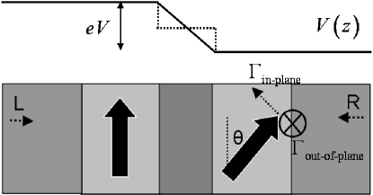
Figure 1: Spin valve showing the different components of torques on a magnetic layer. Bold arrows indicate the direction of magnetization in the two ferromagnetic layers (light grey) surrounded by nonmagnetic material (dark gray). The assumed potential drop is shown above the multilayer: the dark curve shows the linear potential drop used for the numerical results, while the dashed step-like function is the potential drop assumed in analytic formulas. Contributions to the torque are found from states emanating from L and R lead separately.

II Method

The approach we adopt is relevant for systems in the ballistic limit. In the spirit of Landauer’s approach to transport in mesoscopic systems, we suppose the system is connected to two reservoirs (to the left (L) and right (R)) in separate thermal equilibria, with chemical potentials $\mu_{\rm L}$ and $\mu_{\rm R}$. A bias voltage $eV$ across the system is represented by a difference $eV$ between the reservoir chemical potentials. States in the system can be classified as emanating either from the L or R lead (our formalism omits contributions from bound states with energies within the bias window). We find expressions for the interlayer exchange coupling due to states emanating from the L and R lead separately. This permits us to find the interlayer exchange coupling when L and R leads have different chemical potentials (that is, when there is an applied bias).

We utilize a nonequilibrium Green’s function approach, in which the presence of the Left/Right lead is accounted for with a retarded (advanced) self-energy $\Sigma^{r(a)}_{{\rm L/R}}(E)$, and observables are expressed in terms of Green’s functions $G^{r(a)}(E)=\left(E-H-\Sigma^{r(a)}_{\rm L}(E)-\Sigma^{r(a)}_{\rm R}(E)\right)^{-1}$. Our approach generalizes the expressions of Liechtenstein et al. leich to find magnetic exchange interactions for nonequilibrium systems.

When the spins of some subset of orbitals $\{i\}$ are rotated by an angle $\theta$ from their collinear ground state orientation, there will be exchange torques on these orbitals of the form $J=J_{1}\sin(\theta)+J_{3}\sin^{3}(\theta)+...~{}$. Assuming $\mu_{\rm L}>\mu_{\rm R}$, we state here the final result for exchange torque coefficient $J_{1}$ (we defer the derivation, and more details regarding nonequilibrium Green’s functions, to appendix A):

$$J_{1} = \frac{1}{\pi}{\rm Im}\int_{-\infty}^{\mu_{\rm R}}{\rm Tr}\left[\Delta\left(G^{r}_{\uparrow}-G^{r}_{\downarrow}\right)-\Delta G^{r}_{\uparrow}\Delta G^{r}_{\downarrow}\right]dE$$

$$~{}~{}+{\rm Re}\int_{\mu_{\rm R}}^{\mu_{\rm R}+eV}{\rm Tr}\left[\Delta\left(G^{<}_{\uparrow}-G^{<}_{\downarrow}\right)-\right.$$

$$\left.~{}~{}~{}~{}~{}~{}~{}~{}~{}~{}~{}~{}~{}~{}~{}~{}~{}~{}\left(\Delta G^{r}_{\uparrow}\Delta G^{<}_{L,\downarrow}+\Delta G^{<}_{L,\uparrow}\Delta G^{a}_{\downarrow}\right)\right]dE$$

, (1)

where $\Delta=H_{\uparrow}-H_{\downarrow}$ is the spin-dependent Hamiltonian, $G^{<}_{L,\sigma}=\frac{i}{2\pi}G^{r}_{\sigma}\left(\Sigma_{\rm L}^{r}-\Sigma_{\rm L}^{a}\right)_{\sigma}G^{a}_{\sigma}$, and the traces are over orbitals $\{i\}$ that have rotated spins. For ${\rm V}=0$, the limits on the 2nd integral are identical so that its contribution vanishes. In this case Eq. (1) reduces to the well established expression for equilibrium exchange interaction of Ref. leich, . For ${\rm V}\neq 0$, in addition to contributions from the second term of Eq. (1), the bias potential will also alter the Greens functions. Eq. (1) is applicable for both bulk ferromagnets and magnetic multilayers. (In our previous ${\it ab~{}initio}$ work on spin transfer torques in Co-Cu spin valves, we presented only the contribution from the second term of Eq. (1) haney ; heiliger2 .)

As an application of Eq. (1), we consider a one-dimensional, single band tight-binding model of two finite ferromagnetic layers with $n_{{\rm F1}},n_{{\rm F2}}$ sites, separated by a nonmagnetic spacer with $n_{\rm S}$ sites, with nonmagnetic leads. The model is parameterized by the spin-splitting of the ferromagnetic (FM) layers (assumed equal) $\Delta$, a scalar potential in the spacer layer $U$, the Fermi energy $E_{\rm F}$, and the number of layer sites $n_{{\rm F1}},n_{{\rm F2}},n_{{\rm S}}$. $n_{\rm S}$ determines the spacer layer width $D$: $D=a(n_{\rm S}+1)$ for a lattice spacing $a$. Energies are presented in dimensionless form, scaled by the tight-binding hopping parameter $t$. We focus here on some limiting cases in which the physics is clear, and which are relevant for realistic systems. In all of our numerical calculations we assume that the bias potential drop is linear and occurs over the spacer layer (see Fig. (1)), although in our limiting analytic results we neglect this linear potential and assume a step-like potential.

III Results

III.1 Small confinement, large spacer

In the spirit of earlier work on interlayer exchange coupling, we first consider weak spin-dependent potential in the ferromagnet $V_{\uparrow,\downarrow}$, and large spacer thickness $D$. In this limit, the one-dimensional, zero bias interlayer exchange coupling takes the well-established formedwards ; bruno ; stiles :

$$J = \frac{\hbar v_{\rm F}}{2\pi D}{\rm Im}\left[\left(r^{\uparrow}_{1}-r^{\downarrow}_{1}\right)\left(r^{\uparrow}_{2}-r^{\downarrow}_{2}\right)e^{2ik(E_{\rm F})D}\right],$$ (2)

where $r^{\uparrow(\downarrow)}_{1(2)}$ is the reflection off of the spin- up (down) potential of layer 1 (2), and $k(E_{\rm F})$ is the Fermi wave-vector of the spacer layer. $v_{\rm F}$ is the Fermi velocity, given by $v_{\rm F}=\partial E/\hbar\partial k$. (Note that $r^{\uparrow(\downarrow)}_{1(2)}$ includes the thickness dependence of the ferromagnetic layers.) The interpretation of Eq. (2) is that to lowest order in $r$, the two layers are magnetically coupled together via itinerant states in the spacer through spin-dependent reflection of spacer states on both layer 1 and 2, with the mediating state picking up a phase factor $2k(E_{\rm F})D$ for the round trip between the layers. Eq. (2) has been successful in describing the spacer material and thickness dependence of interlayer exchange coupling in experiments stiles ; bruno ; unguris .

At zero bias, the interlayer exchange coupling on layers 1 and 2 is necessarily equal and opposite, because there is no external source of angular momentum. Therefore the choice of rotating layer 1 or 2 to find the interlayer exchange coupling is arbitrary. Under bias, the interlayer exchange coupling on layers 1 and 2 can be different because the reservoirs supply angular momentum when out of equilibrium. This implies that the interlayer exchange torque is not the same on layers 1 and 2. Here we consider the interlayer exchange torque on layer 1. As described in the previous section, we find the torque $J_{\rm L/R}$ due to electrons from the ${\rm L/R}$ lead separately. The calculation of $J_{{\rm L/R}}$ can be found in Appendix B, here we give the result:

$$J_{\rm L} = \frac{\hbar v_{{\rm F}}}{2\pi D}{\rm Im}\left[\left(r^{\uparrow}_{1}-r^{\downarrow}_{1}\right)\left(r^{\uparrow}_{2}-r^{\downarrow}_{2}\right)e^{2ik(E_{\rm F})D}\right],$$

$$J_{\rm R} = 0.$$ (3)

We find that that all of the out-of-plane torque on layer 1 is due to states emanating from L, while states from R contribute nothing. This can be understood in terms of paths of states from L or R considered to second order in the reflectivity in $r$. Fig. (2) shows the relevant path for states from the L and R leads. A state from L transmits through 1, reflects off 2 (so that it now “carries” information about 2), comes back and reflects off 1, effectively “communicating” that information to 1, thereby coupling the two layers. For states from R, the two-reflection path transmits through 2 (so is initially oblivious of it), reflects off 1, comes back and reflects off 2. A final reflection off 1 would communicate spin information from 2, but this would be a third order process. There is therefore no second order contribution to the interlayer exchange coupling on layer 1 with this path.

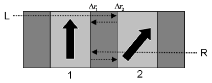
Figure 2: Paths for states emanating from L and R leads for interlayer exchange coupling to lowest order in the spin-dependent reflectivity $\Delta r$.

There are, of course, contributions to both $J_{\rm L}$ and $J_{\rm R}$ that are higher order in the reflectivities. However, in the limit that the reflectivities are much less than one, the additional contributions are negligible.

We assume that the dependence of $J$ on $E_{F}$ is dominated by the exponential factor. (That is, we assume $D\left(\partial k/\partial E\right)$ is much larger than $\partial r/\partial E$ and $~{}(\hbar/JD)(\partial v_{\rm F}/\partial E)$, which is valid in the large $D$ limit). The bias dependence can then easily be found:

$$J(V)=\frac{\hbar v_{{\rm F}}}{2\pi D}{\rm Im}\left[\left(r^{\uparrow}_{1}-r^{\downarrow}_{1}\right)\left(r^{\uparrow}_{2}-r^{\downarrow}_{2}\right)e^{2ik\left(E_{{\rm F}}+eV_{{\rm L}}\right)D}\right],$$ (4)

where $eV_{{\rm L}}$ is the bias potential difference between left lead and spacer layer, and the wave vector $k$ is a function of the argument $E_{\rm F}+eV_{{\rm L}}$. The interlayer exchange coupling is an oscillatory function of the bias $V$, with period $2\pi\hbar v_{{\rm F}}/D$. Fig (3) shows numerical evaluation of Eq. (1) for the 1-dimensional tight binding model, and we find excellent agreement with the approximate $J(V)$ of Eq. (4) in the large $D$ regime. We note that the phase of the oscillation is unconstrained, and is set by model parameters, most experimentally relevantly by $D$.

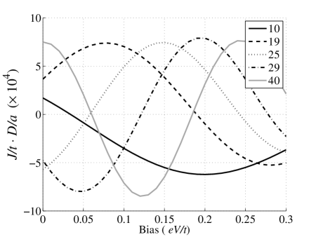
Figure 3: $\left(J/t\cdot~{}D/a\right)$ vs. bias potential for several spacer layer thicknesses. $n_{{\rm F1}}=n_{{\rm F2}}=7,~{}\Delta=0.1t,~{}U=0,~{}E_{\rm F}=-0.78t$ for our 1-d model. Legend shows different spacer widths in units of the lattice spacing $a$.

The success of Eq. (2) in describing experimental data encourages us to believe that Eq. (4) is also experimentally relevant for metallic systems. Making a stationary phase approximation and considering only extremal wave vectors of the Fermi surface, the maximal possible slope of $J(V)$ near 0 bias is:

$${\frac{dJ}{dV}}_{\rm max}=|J_{0}|\frac{De}{\hbar v_{{\rm F}}^{*}}~{},$$ (5)

where $e$ is the electron charge, and $|J_{0}|$ is the maximum equilibrium value (in the 1-d model, $|J_{0}|=\hbar v_{\rm F}|\Delta r_{1}\Delta r_{2}|/2\pi D$), which in this approximation is also related to the value of the coupling at the extremal wave vector, and includes prefactors such as the curvature of the Fermi surface at the extremal point, (see Refs. bruno, ; stiles, for example), and $v_{{\rm F}}^{*}$ is the Fermi velocity of the extremal wave vector. In the case of multiple extremal wave vectors, Eq. (5) should be a sum over all of them. For a Cu spacer with $D=10~{}{\rm nm}$, the change in $J$ is $|J_{0}|0.971~{}{\rm V}$. Assuming the maximum voltage on a metallic multilayer to be on the order of $10^{-4}~{}{\rm V}$, this leads to a maximum change on the order of $10^{-4}|J_{0}|$ (typical values for $J_{0}$ are $0.24~{}{\rm mJ}/{\rm m}^{2},$ bloemen ). We therefore conclude that in metallic systems, the bias-induced change in interlayer exchange coupling is negligible and not measurable.

The oscillatory dependence of the exchange coupling (or out-of-plane torque) on bias may be surprising in light of the general argument for quadratic dependence in symmetric junctions given in Ref. xiao, . It is important to note that this argument assumes semi-infinite ferromagnetic layers, and therefore does not apply to the system under consideration here.

It is instructive at this point to contrast the physics of current-altered interlayer exchange coupling and spin transfer torques. We emphasize that the interlayer exchange coupling properties are dominated by spacer state properties (such as $D$, $k_{\rm F}$, and the curvature of the Fermi surface around extremal points); in this limit, a bias changes interlayer exchange coupling to the extent it changes these spacer state properties. The sensitivity of interlayer exchange coupling to spacer state properties can be motivated by considering the interlayer exchange coupling as resulting from out-of-plane spin currents. For layers 1 and 2 in the $\hat{x}$ and $\hat{z}$ directions respectively, there is no obvious natural preference for the out-of-plane spin current to be in the positive or negative $\hat{y}$ direction. Indeed, the values of out-of-plane spin current for different states are distributed around 0, and mostly cancel. Only around extremal points is there a net contribution (this is why expressions for interlayer exchange coupling involve quantities evaluated only at $E_{\rm F}$ and at extremal wave vectors), and the final value is in some sense accidental. On the other hand, the in-plane torque acting on layer 2 has a strong preference to point in the $x$ direction. As for the out-of-plane torque, the specific values of in-plane torque from different states will vary, but they are distributed now about a nonzero value. For typical metallic systems such as Co-Cu at a current density of $J=10^{8}{\rm A/cm^{2}}$, the magnitude of the out-of-plane torque is $5~{}\%$ that of the in-plane, reflecting this qualitative difference in the spin current vector. This point has been made by Bauer et al. in the language of the mixing conductance $G^{\uparrow\downarrow}$. There the effect is manifest in a small imaginary part of $G^{\uparrow\downarrow}$zwierzycki .

III.2 Half-metal

In this section we take the limit of a metallic junction with half-metallic FM layers. We choose this system because it most easily demonstrates the opposite limit of the small confinement case. We find that in the half-metallic case, electrons from the L and R leads contribute equally to the interlayer exchange coupling on each layer (whereas in the small confinement case, electrons from only one lead contributed to the interlayer exchange coupling). Here we assume the potential for majority channel is flat throughout the magnetic and nonmagnetic layers, and the minority potential is infinite in the ferromagnet. The out-of-plane torque coefficient (near antiparallel alignment, or $\theta\approx\pi$) then takes the simple form:

$$J_{{\rm L,R}}=\frac{1}{2\pi}\int_{-\infty}^{\mu_{{\rm L,R}}}\sin\left[2k\left(E\right)D\right]dE~{},$$ (6)

This expression can be found by computing the out-of-plane spin current in the spacer layer. Integrating over all energies leads to the exact result for the interlayer exchange coupling:

$$J_{{\rm L,R}} = \frac{2v_{\rm F}\hbar(D/a^{2})\cos(2k_{F}D)+E_{\rm F}\sin(2k_{F}D)}{4(D/a)^{2}-1}.$$ (7)

The bias dependence is given by simply shifting the energies of L and R electrons by $+V/2$ and $-V/2$, respectively, leading to:

$$J(V) = J_{\rm L}\left(E_{{\rm F}}+\frac{V}{2}\right)+J_{\rm R}\left(E_{{\rm F}}-\frac{V}{2}\right)$$ (8)

$$\approx J(0)+\frac{1}{2}\frac{\partial^{2}J\left(E_{\rm F}\right)}{\partial E^{2}}\left(\frac{V}{2}\right)^{2}~{}.$$

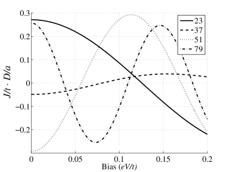
Figure 4: $\left(J/t\cdot~{}D/a\right)$ vs. bias potential for several spacer layer thicknesses. $n_{{\rm F1}}=n_{{\rm F2}}=7,~{}E_{\rm F}=-0.78t$. FM are half metals and results are for $\theta$ near $\pi$. Legend shows different spacer widths in units of the lattice spacing $a$.

Fig. 4 shows numeric results of the bias dependent interlayer exchange coupling for a number of spacer widths. We find these results correspond well with Eq. (8). The curves for interlayer exchange coupling are again periodic in $V$, with the same period $2\pi\hbar v_{{\rm F}}/D$ as the previous small $r$ case. In contrast to the small $r$ case, the phase of the oscillations are constrained so that all curves are $\cos$-like, which leads to a quadratic dependence of the exchange torque at small $V$.

The half-metallic system is emblematic of the general fact that if states from the L and R leads contribute equally to the interlayer exchange coupling, and if there is a symmetric bias potential drop, then the bias dependence of the out-of-plane torque must be quadratic. Mathematically this quadratic dependence is seen immediately from Eq. (8). A physical description is that when a bias $eV$ is applied, we gain contributions from L states at energies above the original Fermi energy (from $E_{\rm F}$ to $E_{\rm F}+\frac{eV}{2}$), while we lose contributions from a lack of R states at energies below the original Fermi energy (from $E_{\rm F}-\frac{eV}{2}$ to $E_{\rm F}$) (see Fig. (5)).

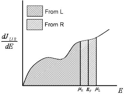
Figure 5: Schematic of how bias potential changes the contributions from the L and R leads to the total interlayer exchange coupling. At zero bias both L and R are contribute equally up to $E_{\rm F}$, while a symmetric bias drop of $eV$ opens a window from $E_{\rm F}-eV/2$ to $E_{\rm F}+eV/2$ with only one lead contributing. This leads to a quadratic dependence of the coupling on the bias.

This gain and loss cancel each other to linear order in $eV$, and only a quadratic dependence remains ralphreview . It should be noted that in making a constant shift in energies of the left and right leads relative to the spacer layer, there are also changes in the contribution from the bottom of the bands. However near the bottom of the band, the contributions to $\Gamma_{\perp}$ oscillate rapidly and don’t contribute (due to a large $\frac{\partial k}{\partial E}$), so that shifts in this region are unimportant. The quadratic dependence of the out-of-plane torque is also discussed in Refs. xiao, ; theodonis, for the case of semi-infinite ferromagnetic layers.

III.3 Tunneling

We next consider the case of a tunneling barrier with half-metallic ferromagnetic layers. Such a model system is relevant for the states at the Brouillon zone center of Fe-MgO-Fe. These states make the dominant contribution to the transport butler , spin torques heiliger , and interlayer exchange coupling mgOinterlayer exchange coupling . An exact expression for the out-of-plane torque is given in Ref. slonc89, for a trilayer (FM leads separated by a spacer); for our 5-layer geometry, $\Gamma_{\perp}$ is generally a complicated function of model parameters. We find that in the symmetric system ($n_{{\rm F1}}=n_{{\rm F2}}$), electrons from both L and R leads contribute equally to the interlayer exchange coupling, so that there is a quadratic dependence of the interlayer exchange coupling on bias voltage, as discussed in the previous section. We make a simplifying ansatz here for $J_{{\rm L/R}}$ and compare its prediction to the $V^{2}$ prefactor with the exact numerical results. We find that our approximate, analytic form shows qualitative agreement with the numerics.

We suppose that the energy dependence of the out-of-plane torque is dominated by the tunneling exponential:

$$J_{{\rm L,R}}=\int_{-\infty}^{\mu_{{\rm L,R}}}Ae^{-2\kappa\left(E\right)D}dE~{},$$ (9)

where $\kappa$ is the decay constant (or imaginary wave-vector) in the spacer. In our model, $\kappa a={\rm Im}\left[\cos^{-1}\left(\left(E_{{\rm F}}-U\right)/2t\right)\right]$. $A$ is a complicated function of model parameters, and we have found that compared to the exponential factor, $A$ depends weakly on energy; we therefore omit its energy dependence going forward. To find the interlayer exchange coupling, we assume energies near the Fermi level make the dominant contribution to the total, leading to:

$$J_{{\rm L,R}}=\frac{At\sinh\left(\kappa_{\rm F}a\right)}{D^{\prime}}e^{-2\kappa_{\rm F}D}~{}.$$ (10)

where $D^{\prime}=D/a$. The bias-dependent interlayer exchange coupling can be written in the form:

$$J(V)=J(0)\left(1+BV^{2}\right).$$ (11)

A straightforward calculation leads to :

$$B = \frac{2D^{\prime 2}-D^{\prime}\coth(\kappa a)-\frac{1}{2}~{}{\rm sech}^{2}(\kappa a)}{8t^{2}\sinh^{2}(\kappa a)}~{}.$$ (12)

In Fig. 6, we plot the logarithm of the $V^{2}$ prefactor for both exact numerical results and for the approximation given above, as a function of $D/a$. The agreement is good, given the fact that we neglect the deformation of the barrier due to the external bias potential in our approximation, and the qualitative trend is correct. Fig. 7 shows the prefactor as a function of Fermi level, and again we find qualitative agreement. The prefactor is exponentially sensitive to system parameters, due to the fact that it is proportional to $J(0)$; the dependence of $B$ on system parameters is much weaker.

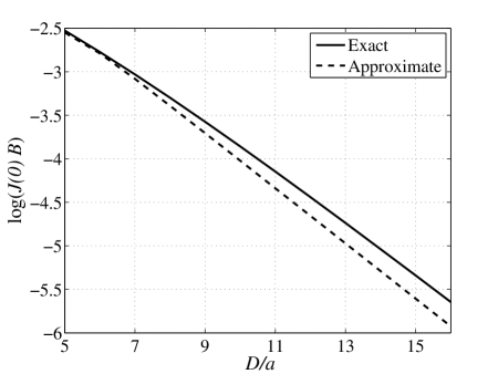
Figure 6: Logarithm of quadratic bias-dependence prefactor versus spacer thickness $D$. Parameters are $U=1.75t,E_{{\rm F}}=-0.4t,n_{{\rm F1}}=n_{{\rm F2}}=7$.

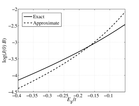
Figure 7: Logarithm of quadratic bias-dependence prefactor versus Fermi energy. Parameters are $U=1.75t,D/a=7,n_{{\rm F1}}=n_{{\rm F2}}=7$.

For all parameters we’ve considered, we find that the zero bias exchange coupling between layers is antiferromagnetic in the tunneling regime, and that the application of a bias increases this antiferromagnetic coupling (i.e., the sign of the $V^{2}$ prefactor is the same as the sign of $J(0)$).

Recent experiments on MgO indicate that at bias potentials on the order of $0.5~{}{\rm V}$, the in-plane and out-of-plane torques are of similar magnitude, in stark contrast to metallic systems in which $\Gamma_{\parallel}\gg\Gamma_{\perp}$. The origin of this difference is the reduced area in $k$-space for the in-plane torque in Fe-MgO. In metals all of the states in the Brouillon zone contribute to the in-plane torque and only states near extremal points of the Fermi surface contribute to the out-of-plane torque, while in Fe-MgO only states near the $\Gamma$ contribution to both in-plane and out-of-plane torques.

IV Conclusion

In this work, we have derived a general expression for magnetic exchange interactions that is valid in nonequilibrium systems in the ballistic regime. We applied this formula to magnetic spin valves to study how the interlayer exchange coupling depends on an external bias voltage. We find that for metallic systems in the small confinement limit, the interlayer exchange coupling is an oscillatory function of the bias, but that the period of the oscillations is so long that seeing a change in interlayer exchange coupling is not experimentally feasible. For tunneling systems, and for any system in which electrons emanating from the L and R leads contribute equally to the interlayer exchange coupling and there is a symmetric bias potential drop, we find that the interlayer exchange coupling depends quadratically on the bias voltage, which is in agreement with recent experiments.

We emphasize that the results we obtain are for systems in the ballistic regime. The behavior of $\Gamma_{\perp}(V)$ for systems in the diffusive regime is generally different. In particular, a nonzero $\Gamma_{\perp}$ at zero bias is a phase coherent effect; diffusive systems have a vanishing equilibrium $\Gamma_{\perp}$. The oscillatory $V$-dependence described for metallic systems is derived from modulating the wave-vector of coherent states, and will not be seen for diffusive systems. Diffusive systems under bias generally have a nonzero $\Gamma_{\perp}$. For symmetric systems, this dependence is quadratic and is therefore omitted from purely linear theories such as the spin circuit theory brataas . For asymmetric structures, there is a linear contribution to $\Gamma_{\perp}(V)$, which is described by linear, diffusive theories, where for example in the spin circuit theory it is related to the imaginary part of the mixing conductance

There are other systems in which bias-altered exchange interactions can have important effects. It is possible, for example, that in single ferromagnetic layers under bias, intralayer exchange interactions can be affected by this bias, which would be manifest in a change of spin wave dispersion or Curie temperature. We are currently investigating these types of systems.

*

Appendix A Expansion of nonequilibrium density matrix in magnetic rotations

Here we describe in more detail the calculation of exchange interactions in systems under bias. Our approach is based on the nonequilibrium Green’s function method. In this method, we assume there is some central region, described by a Hamiltonian $H_{\rm C}$, embedded between two semi-infinite reservoirs or leads. The left and right leads are described by the semi-infinite Hamiltonians $H_{\rm L}$ and $H_{\rm R}$ respectively. We denote the coupling between the central region and the left/right leads by $\tau_{L}$/$\tau_{R}$. The retarded Green’s function for the isolated central region is simply $G_{\rm C}^{r}(E)=\left(E+i\eta-H_{\rm C}\right)^{-1}$. The presence of the left lead is accounted for with self-energy $\Sigma_{\rm L}(E)=\tau_{\rm L}g_{\rm L}^{r0}\tau_{\rm L}^{\dagger}$, where $g_{\rm L}^{r0}=\left(E+i\eta-H_{\rm L}\right)^{-1}_{0,0}$ is the so-called surface Green’s function. This is the projection of the full semi-infinite lead Green’s function onto the subset of lead sites which couple to the central region (for the one-dimensional model we consider, this subset is denoted as the $({0,0})$ element of the full left lead Green’s function). The self-energy for the right lead is defined similarly. The total retarded Green’s function for the center region plus leads is then $G^{r}(E)=\left(E+i\eta-H_{\rm C}-\Sigma_{\rm L}^{r}-\Sigma_{\rm R}^{r}\right)^{-1}$. In the following we combine left and right self energies: $\Sigma^{r,a}\equiv\Sigma_{\rm L}^{r,a}+\Sigma_{\rm R}^{r,a}$.

The so called “lesser” Green’s function is given by the well-known Keldysh equation : $G^{<}=\frac{1}{2\pi}G^{r}\Sigma^{<}G^{a}$haug ; datta , where $\Sigma^{<}_{\rm L/R}=i\left(\Sigma^{r}_{\rm L/R}-\Sigma^{a}_{\rm L/R}\right)$. The contribution to the density matrix from states emanating from the L/R lead is:

$$\rho_{\rm L/R} = \int_{-\infty}^{E_{\rm F}}G_{\rm L/R}^{<}(E)~{}dE$$ (13)

$$= \frac{1}{2\pi}\int_{-\infty}^{E_{\rm F}}G^{r}\Sigma^{<}_{\rm L/R}G^{a}dE.$$ (14)

We consider how the density matrix changes upon the addition of some perturbation $H^{\prime}$ to the Hamiltonian. To this end we consider how the integrand of Eq. (14) changes, and omit the energy integral for clarity. The integrand is given more explicitly as:

$$G^{<}=\frac{1}{2\pi}\left(\frac{1}{E-H_{\rm C}-\Sigma^{r}}\right)\Sigma^{<}\left(\frac{1}{E-H_{\rm C}-\Sigma^{a}}\right).$$ (15)

We restrict our attention to perturbations $H^{\prime}$ which are only present in the central region; $H^{\prime}$ leads to a new Green’s function $G^{<}_{1}$, given by:

$$G^{<}_{1} = \frac{1}{2\pi}\left(\frac{1}{E-H_{\rm C}-H^{\prime}-\Sigma^{r}}\right)\Sigma^{<}\left(\frac{1}{E-H_{\rm C}-H^{\prime}-\Sigma^{a}}\right).$$

To first order in $H^{\prime}$, $G^{<}_{1}$ is:

$$G^{<}_{1} \approx \frac{1}{2\pi}~{}G^{r}(1+H^{\prime}G^{r})\Sigma^{<}G^{a}(1+H^{\prime}G^{a})$$ (17)

$$\approx G^{<}+G^{r}H^{\prime}G^{<}+G^{<}H^{\prime}G^{a}.$$

All of these objects are represented in a real-space basis, and we consider perturbations about a collinear ground state. The components of the unperturbed Green’s functions are then labeled with site index $i,j$, and are diagonal in spin space:

$$G_{i,j}=\left(\begin{array}[]{cc}G_{\uparrow,i,j}&0\\ 0&G_{\downarrow,i,j}\\ \end{array}\right).$$ (20)

In all $2\times 2$ matrices, we indicate explicitly site labels with indices and also spin label. As before, we define $\Delta_{i,j}=\delta_{i,j}\frac{1}{2}\left(H_{\uparrow}-H_{\downarrow}\right)_{i,j}$. We consider tilting some portion (sites $\{i^{\prime}\}$) of the magnetization by a small angle $\theta$, so that $H^{\prime}$ is given by:

$$H^{\prime}_{i,i}=\sum_{i\in\{i^{\prime}\}}\frac{\Delta_{i,i}}{2}\left(\begin{array}[]{cc}\cos(\theta)-1&\sin(\theta)\\ \sin(\theta)&1-\cos(\theta)\\ \end{array}\right)~{}.$$ (23)

There can in principle be spin-dependent terms that are off-diagonal in site index, but these are usually much smaller than site-diagonal terms and omitted here. Inserting Eq. (23) into Eq. (17) yields:

$$G^{<}_{1}-G^{<}=$$

$$~{}~{}\frac{1}{2}\left[\begin{array}[]{cc}G^{r}_{\uparrow}(\cos(\theta)-1)\Delta^{\prime}G^{<}_{\uparrow}&G^{r}_{\uparrow}\sin(\theta)\Delta^{\prime}G^{<}_{\downarrow}\\ G^{r}_{\downarrow}\sin(\theta)\Delta^{\prime}G^{<}_{\uparrow}&G^{r}_{\downarrow}(1-\cos(\theta))\Delta^{\prime}G^{<}_{\downarrow}\\ \end{array}\right]+{\rm h.c.}$$ (26)

Where for notational clarity we’ve introduced matrices $\Delta^{\prime}$, where $\Delta^{\prime}_{i,i}=\Delta_{i,i}$ if $i\in\{i^{\prime}\}$, and 0 otherwise. In the above h.c. stands for “Hermitian conjugate”. From the perturbed density matrix we find the ensuing spin densities (to first order in $\theta$):

$$m_{i,j}^{x} = 2\theta~{}{\rm Re}\left[(G^{r}_{\uparrow}\Delta^{\prime}G^{<}_{\downarrow}+G^{r}_{\downarrow}\Delta^{\prime}G^{<}_{\uparrow})\right]_{i,j}$$

$$m_{i,j}^{y} = 2\theta~{}{\rm Im}\left[(G^{r}_{\uparrow}\Delta^{\prime}G^{<}_{\downarrow}-G^{r}_{\downarrow}\Delta^{\prime}G^{<}_{\uparrow})\right]_{i,j}$$

$$m_{i,j}^{z} = \left(G^{<}_{\uparrow}-G^{<}_{\downarrow}\right)_{i,j}+O\left(\theta^{2}\right)~{}.$$ (28)

As discussed in the introduction, the exchange torques in a multilayer can be found by computing the out-of-plane torque. These torques result from the misalignment between the spin-dependent Hamiltonian and the spin density. To find this misalignment, we need the vector components of the spin-dependent perturbed Hamiltonian $H+H^{\prime}$, given as: $\Delta_{\alpha}={\rm Tr}\left[\left(H+H^{\prime}\right)\sigma_{\alpha}\right],~{}\{\alpha=x,y,z\}$, where $\sigma_{\alpha}$ are Pauli spin matrices. If the layers’ magnetizations span the $x-z$ plane, then the exchange torque is:

$$\Gamma_{y}=\Delta_{x}m_{z}-\Delta_{z}m_{x}~{}.$$ (29)

Expanding to first order in $\theta$ leads to the following expression for the coupling due to states from the L/R leads:

$$J_{{\rm L/R}} = {\rm Re}~{}\int_{-\infty}^{\mu_{\rm L/R}}{\rm Tr}\left[\Delta^{\prime}\left(G^{<}_{\uparrow\rm L/R}-G^{<}_{\downarrow\rm L/R}\right)-\right.$$

$$\left.\left(\Delta^{\prime}G^{r}_{\uparrow}\Delta^{\prime}G^{<}_{\downarrow\rm L/R}+\Delta^{\prime}G^{r}_{\downarrow}\Delta^{\prime}G^{<}_{\uparrow\rm L/R}\right)\right]dE~{}.$$

In equilibrium, the total lesser Green’s function $G^{<}=G^{<}_{L}+G^{<}_{R}$ can be written in terms of the retarded Green’s function alone: $G^{<}=\frac{i}{2\pi}\left(G^{r}-G^{a}\right)$, in which case the expression for the total exchange torque becomes:

$$J=\frac{1}{\pi}{\rm Im}\int_{-\infty}^{E_{\rm F}}{\rm Tr}\left[\Delta^{\prime}\left(G^{r}_{\uparrow}-G^{r}_{\downarrow}\right)-\Delta^{\prime}G^{r}_{\uparrow}\Delta^{\prime}G^{r}_{\downarrow}\right]dE~{}.$$

(31)

Combining Eq. (31) for energies in which both leads are occupied, and Eq. (LABEL:eq:jneq) for energies in which only one lead is occupied yields Eq. (1).

We should note that in using the non-self-consistent spin density from a system rotated slightly out of collinearity to find torques, we are implicitly making use of the magnetic force theorem. In addition, we utilize the same assumptions as Ref. leich, , namely that the orientation of spin magnetic moments on each lattice site is a well-defined quantity, and that these spin orientation degrees of freedom are “slow” with respect to the electronic degrees of freedom (adiabatic approximation). The validity of these approximations have been considered in detail in previous works antropov .

We make some final comments to compare our result for exchange interactions with previous equilibrium expressions for exchange interactions. First, in similar spirit to Ref. leich, , we can attempt to define the pairwise interaction of two spins $J_{i,j}$ by finding the exchange torque present on atom $i$ when $i$ and $j$ are both rotated, and subtracting off the torques present on $i$ when $i$ and $j$ are rotated separately. Under nonequilibrium conditions however, the following sum rule is violated:

$$J_{i}\neq\sum_{j\neq i}J_{ij}.$$ (32)

implying that a pairwise interaction is not properly defined in nonequilibrium conditions. This is again due to the fact that there is a net flux of angular momentum into the system from the current-carrying electrons.

Finally we note that the approach taken in Ref. leich, to finding exchange interactions relies on calculating the change in single particle energy $\Delta E$ upon rotating a portion of the magnetism away from collinearity. It can be shown that in equilibrium, this change in energy can be expressed in the language of Greens functions as:

$$\Delta E=\frac{1}{2}{\rm Tr}\left[H^{\prime}\left(\rho^{\prime}+\rho\right)\right]~{}.$$ (33)

where $\rho^{\prime}$ is the density matrix corresponding to the perturbed lesser Green’s function $G^{<}_{1}$. We have found that this expression works in nonequilibrium conditions as well, and gives identical results to the exchange torques found using spin densities.

A.1 In-plane torques

With the expansion of the nonequilibrium density matrix given by Eqn. (17), it is a simple matter to find the spin transfer torque, which we do here for completeness. As in Ref. haney, , we find the out-of-plane spin density to determine the spin transfer torque present on a subsystem of atoms $\{j\}$, when atoms $\{i^{\prime}\}$ are rotated by a small angle $\theta$. Assuming the two layers span the $x-z$ plane, the $y$-component of the spin density is called for: the out-of-plane spin density in a spin valve determines the spin torques. The spin transfer torque is thus $\Gamma^{IP}=|\Delta|m_{y}$. As before, we use the expansion of $\vec{m}$ given by Eq. (28) to obtain:

$$\frac{\Gamma^{IP}}{\sin(\theta)} = \frac{\mu_{B}}{\hbar}~{}{\rm Im}\int_{\mu_{\rm R}}^{\mu_{\rm R}+eV}~{}{\rm Tr}\left[\Delta^{\prime}G^{r}_{\uparrow}\Delta^{\prime\prime}G^{<}_{\downarrow}-\right.$$ (34)

$$~{}~{}~{}~{}~{}~{}~{}~{}~{}~{}~{}~{}~{}~{}~{}~{}\left.\Delta^{\prime}G^{r}_{\downarrow}\Delta^{\prime\prime}G^{<}_{\uparrow}\right]dE~{}.$$

Where the trace is over orbitals of the subsystem $\{j\}$ in question, $\Delta^{\prime}$ and $\Delta^{\prime\prime}$ are the spin-dependent Hamiltonian for orbital sets $\{j\}$ and $\{i\}$, respectively. Eq. (34) has the utility of expressing in plane torques in terms of collinear objects, simplifying the numerical task of calculating these torques from first principles relative to calculating full noncollinear spin configurations, as in Refs. haney, and heiliger2, .

A.2 Bias dependence of interlayer exchange coupling

Here we take the limit of large spacer thickness and small reflectivities, and reformulate $J$ in the language of Refs. stiles, and bruno, . We consider first the equilibrium case as a precursor to the nonequilibrium case. We can rewrite the Green’s functions in terms of free space Green’s functions $G_{0}$:

$$G^{r} = G_{0}^{r}+G_{0}^{r}(T_{A}+T_{B})G_{0}^{r}~{},$$ (35)

$$G_{0_{(j,j^{\prime})}}^{r} = \frac{e^{ik|j-j^{\prime}|}}{i\hbar v_{k}}~{},$$ (36)

$$T_{A,B} = \frac{V_{A,B}}{1-G^{r}_{0}V_{A,B}}~{}.$$ (37)

$T$ includes the influence of the potentials $V_{A,B}$ exactly. When the potentials $V$ is small, then $T\approx V$ and $G$ is approximately given as:

$$G^{r} = G_{0}^{r}+G_{0}^{r}(V_{A}+V_{B})G_{0}^{r}~{}.$$ (38)

Inserting Eq. (38) into Eq. (31) and retaining the lowest order terms in $V$ leads to a useful form of $J$:

$$J = \frac{1}{\pi}{\rm Im}~{}{\rm Tr}\int\left(V_{B}^{\uparrow}-V_{B}^{\downarrow}\right)G_{0}\left(V_{A}^{\uparrow}-V_{A}^{\downarrow}\right)G_{0}dE~{}.$$

In the spirit of previous works on interlayer exchange coupling, we next rewrite Eq. (A.2) in terms of spin-dependent reflectivities of the magnetic layers. The effect of a single potential $V_{A,B}$ is described by the reflection and transmission coefficients $r_{A,B}$ and $t_{A,B}$. We suppose the potential to be confined to sites $i$ within a range $i\in\{i^{\prime}\}$, and that the “left-most” site is $i_{L}$. For our purposes, it suffices to consider the change in Green’s function $\delta G_{i,j}$ induced by the potential for indices $i,j$ on the same “side” of the potential, i.e. $i,j<i_{L}$. Then, for small $V_{A}$ (see Fig. (8)):

$$\delta G_{i,j} = \left(G_{0}T_{A}G_{0}\right)_{i,j}$$ (40)

$$= i\hbar v_{k}G_{0_{(i,i_{L})}}r_{A}~{}G_{0_{(i_{L},j)}}~{}.$$

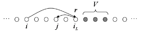
Figure 8: Schematic for effect of potential V on $G_{i,j}$: the path from site i to site j can contain a reflection $r$ off of the left edge of the potential V.

Using the fact that $V_{A,B}\approx T_{A,B}$, applying Eq. (40) twice, and the form for $G_{0}$ given in Eq. (36) leads to:

$$J = \frac{1}{\pi}{\rm Im}\int\left(r^{\uparrow}_{A}-r^{\downarrow}_{A}\right)\left(r^{\uparrow}_{B}-r^{\downarrow}_{B}\right)e^{2ik_{\rm F}D}~{}dE~{}.$$

where $D=a\left(n_{\rm S}+1\right)$. For the nonequilibrium case, we insert Eq. (38) into Eq. (LABEL:eq:jneq), and keep lowest order in $V$:

$$J_{{\rm L,R}} = \frac{1}{\pi}{\rm Im}\int_{-\infty}^{\mu_{L,R}}\left(V^{\uparrow}_{B}-V^{\downarrow}_{B}\right)\left(G_{0}^{r}\Gamma_{L,R}G_{0}^{a}\left(V^{\uparrow}_{A}-V^{\downarrow}_{A}\right)G_{0}^{a}\right.$$ (42)

$$~{}~{}~{}~{}~{}\left.+G_{0}^{r}\left(V^{\uparrow}_{A}-V^{\downarrow}_{A}\right)G_{0}^{r}\Gamma_{L,R}G_{0}^{a}\right)dE~{}.$$

In terms of reflectivities and phase factors, this becomes:

$$J_{\rm L} = 0~{},$$

$$J_{\rm R} = \frac{1}{\pi}\textrm{Im}\int_{-\infty}^{\mu_{R}}\left[\left(r^{\uparrow}_{A}-r^{\downarrow}_{A}\right)\left(r^{\uparrow}_{B}-r^{\downarrow}_{B}\right)e^{2ikD}\right]dE~{}.$$

Evaluating the integral in the large $D$ limit leads to Eq. (3) of the text.

References

- (1) M. D. Stiles, Nanomagnetism: Ultrathin Films, Multilayers and Nanostructures (Contemporary Concepts of Condensed Matter Science, Vol 1), eds. D. Mills and J. A. C. Bland, New York: Elsevier, 2006 pp 51-77.
- (2) M.D. Stiles, Ultrathin Magnetic Structures III, eds. B. Heinrich and J.A.C. Bland, (Springer-Verlag, Berlin, 2004).
- (3) S. S. P. Parkin, N. More, and K. P. Roche, Phys. Rev. Lett., 64, 2304 1990.
- (4) J. Unguris, R. J. Celotta, and D. T. Pierce, Phys. Rev. Lett., 79, 2734 (1997).
- (5) D. M. Edwards and J. Mathon, J. Magn. Magn. Mat. 93, 85 (1991).
- (6) P. Bruno, Phys. Rev. B 52, 411 (1995).
- (7) M. D. Stiles, Phys. Rev. B 48, 7238 (1993).
- (8) A. I. Liechtenstein, M. I. Katsnelson, V. P. Antropov, and V. A. Gubanov, J. Magn. Magn. Mat. 67, 65, (1986).
- (9) J. C. Slonczewski, Phys. Rev. B 39, 6995 (1989).
- (10) J. C. Slonczewski, J. Magn. Magn. Mat. 62, 123 (1996).
- (11) L. Berger, Phys. Rev. B 54, 9353 (1996).
- (12) In equilibrium, a spin valve with layer magnetizations in the plane is invariant under the combined operations of time reversal + spin rotation by about the axis. Out-of-plane torques are also invariant under this operation and are therefore allowed by symmetry, while in-plane torques are not, and therefore vanish. The application of a current breaks time-reversal symmetry, allowing a non-zero in-plane torque. Similar arguments can be made for general magnetization textures in equilibrium and non-equilibrium.
- (13) A. A. Tulapurkar, Y. Suzuki, A. Fukushima, H. Kubota, H. Maehara, K. Tsunekawa, D. D. Djayaprawira, N. Watanabe and S. Yuasa, Nature 438, 339 (2005).
- (14) J. C. Sankey, Yong-Tao Cui, J. Sun, J. Slonczewski, R. A. Buhrman, and D. C. Ralph, Nature Phys. 4, 67 (2008).
- (15) M. A. Zimmler, B. Özyilmaz, W. Chen, A. D. Kent, J. Z. Sun, M. J. Rooks, and R. H. Koch, Phys. Rev. B 70, 184438 (2004).
- (16) P. M. Haney, D. Waldron, R. A. Duine, A. S. Núñez, H. Guo, and A. H. MacDonald, Phys. Rev. B 76, 024404 (2007), 77 059901(E) (2008).
- (17) C. Heiliger, M. Czerner, B. Yu. Yavorsky, I. Mertig, and M. D. Stiles, J. Appl. Phys. 103, 07A709 (2008).
- (18) J. C. Slonczewski, Phys. Rev. B 71, 024411 (2005).
- (19) I. Theodonis, N. Kioussis, A. Kalitsov, M. Chshiev, and W. H. Butler, Phys. Rev. Lett. 97, 237205 (2006).
- (20) J. Xiao, G. E. W. Bauer, and A. Brataas, Phys. Rev. B 77, 224419 (2008).
- (21) V. I. Kozub and V. Vinokur, App. Phys. Lett. 87, 062507 (2005).
- (22) N. F. Schwabe, R. J. Elliott, and Ned S. Wingreen, Phys. Rev. B 54, 12953 (1996).
- (23) C. Heide, P. E. Zilberman, and R. J. Elliott, Phys. Rev. B 63, 064424 (2001).
- (24) P. J. H Bloemen, M. T. Johnson, M. T. H. van de Vorst, R. Coehoorn, J. J. de Vries, R. Jungblut, J. aan de Stegge, A. Reinders, and W. J. M. de Jonge, Phys. Rev. Lett. 72, 764 (1994).
- (25) M. Zwierzycki, Y. Tserkovnyak, P. J. Kelly, A. Brataas, and G. E. W. Bauer, Phys. Rev. B 71, 064420 (2005).
- (26) D. C. Ralph and M. D. Stiles, J. Magn. Magn. Mat. 320, 1190 (2008).
- (27) W. H. Butler, X.-G. Zhang, T. C. Schulthess, and J. M. MacLaren, Phys. Rev. B 63, 054416 (2001).
- (28) C. Heiliger and M. D. Stiles, Phys. Rev. Lett. 100, 186805 (2008).
- (29) T. Katayama and S. Yuasa, App. Phys. Lett. 89, 112503 (2006).
- (30) A. Brataas, G. E. W. Bauer, and P. J. Kelly, Phys. Rep. 427, 157 (2006).
- (31) H. Haug and Antti-Pekka Jauho, Quantum kinetics and optics of Semiconductors. Springer Verlag, 1996.
- (32) S. Datta, Electronic Transport in Mesoscopic Systems. Cambridge University Press, 1995.
- (33) V.P. Antropov, B.N. Harmon, and A.N. Smirnov, J. Magn. Magn. Mat. 200, 148 (1999).