Asymptotic Entanglement Dynamics and Geometry of Quantum States

Abstract

A given dynamics for a composite quantum system can exhibit several distinct properties for the asymptotic entanglement behavior, like entanglement sudden death, asymptotic death of entanglement, sudden birth of entanglement, etc. A classification of the possible situations was given in [M. O. Terra Cunha, New J. Phys 9, 237 (2007)] but for some classes there were no known examples. In this work we give a better classification for the possibile relaxing dynamics at the light of the geometry of their set of asymptotic states and give explicit examples for all the classes. Although the classification is completely general, in the search of examples it is sufficient to use two qubits with dynamics given by differential equations in Lindblad form (some of them non-autonomous). We also investigate, in each case, the probabilities to find each possible behavior for random initial states.

I Introduction

Entanglement is a fundamental property of composite quantum systems, first noted by Schrödinger schroedinger . The best knowledge of the whole of a composite quantum system may not include complete knowledge of its parts. It has strong conceptual implications on physics, since it is a property that has no classical analog, so we are forced to change significantly our perspective of Nature. Such peculiar character allows it to be considered as a fundamental resource for some non-classical tasks as teleportation of a quantum state teleporte , quantum computation quantumcomp , quantum cryptography ekert , etc . Once entanglement is considered a resource it seems natural to quantify it entanquant . In all the applications named above, it is necessary to optimize the amount of entanglement in a suitable composite quantum system to best execute the desired task.

Real quantum systems always interact with its environment, irrespectively of the efforts to protect it. This interaction will, in general, create some entanglement between the quantum system and the environment, and this entanglement will, somewhat ironically, spoil the entanglement between the parts of the “useful” system (for bipartite systems, this affirmation has a precise meaning provided by the monogamy of entanglement theorem monogamy ).

While in most of the models used to describe quantum open systems the coherences of a state decays asymptotically to zero, it was recently recognized that entanglement may “die” at finite time primeiramorte , a phenomenon called entanglement sudden death eberlyesd . This phenomenon has called some attention, specially connected to the difficulty of keeping entanglement alive for its uses as a resource. Some interesting generalizations were studied gen , and some experiments were proposed proposta and realized experimentodavidov . This phenomena, though, has a simple explanation if one looks at the geometry of quantum states terra . Namely, while the set of “decohered” states always have zero volume inside the set of all possible quantum states, the set of separable states has not only a positive volume but also non-empty interior volume when the global system have a finite dimensional Hilbert space.

The geometrical approach to the problem allows one to classify the dynamics of a quantum system according to the geometry of its asymptotic states (if the dynamics implies them) relative to the set of separable states terra . In the cited paper some classes were exemplified, but to that time it was not clear whether all a priori possible situations could be found.

In this paper we review the geometric classification of entanglement dynamics and provide explicit examples to all a priori possible situations. All examples are given in the two-qubit Lindblad differential equations context, with some cases using non-autonomous equations (exactly those in the classes for which examples were not previously known). We also introduce a new analysis of how often each specific behavior occur for a given dynamics, in the light of probability theory applied to the set of initial states viviescas .

II The Geometry of Entanglement Sudden Death: General Picture

What can we say about the geometry of entanglement, or the geometry of the set of separable states, for general multipartite systems? First of all, that the set of separable states is closed, convex and with non-empty interior (we shall assume finite dimensional Hilbert spaces throughout the paper). Its complement relative to the set of quantum states also has non-empty interior and is certainly non-convex. Actually, in general, its complement is much larger, i.e., it has greater volume (if one consider the Hilbert-Schmidt metric, for instance). An extremely oversimplified illustration of this situation is given in Fig. 1. We call here $D$ the set of all quantum states and we are going to consider it immersed in the set $\mathcal{A}$ of Hermitian matrices of unity trace; $S$ the subset composed by the separable states, $\partial S$ and $\partial D$ their boundaries relative to $D$ and $\mathcal{A}$, respectively; $E=D-S$ the set of entangled states. The boundary of the set of quantum states is composed by all that states which have at least one zero eigenvalue so, in particular, it contains all the pure states. Note that there are both entangled and separable pure states in $\partial D$. Actually, more than that, the “area” of the separable states inside $\partial D$ is non-zero artigojgp .

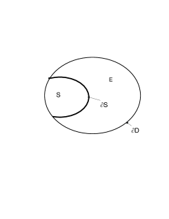
Figure 1: Diagram of the set of entangled states.

Let us consider a dynamics with a non-trivial stationary set, $St$. By stationary set we mean that for every initial state $\rho$ and open set $V\supseteq St$ we have that $\rho(t)$ (the state at time $t$) belongs to $V$ for all $t$ sufficiently large. Of course, if some dynamics accepts a set of stationary states, this set will be the smallest stationary set of the dynamics. Anyway, from the simple picture given in Fig. 1, and considering the location of $St$ in it, we may distinguish three possibilities which have consequences to the asymptotic dynamics of entanglement: i) $St\subset\text{ Int}(S)$ implies that every initial entangled state will lose all of its entanglement at finite time (sudden death of entanglement); ii) if $St\cap\partial S\neq\emptyset$, than, only with that information, many situations can occur: asymptotic or sudden death of entanglement and non-zero asymptotic entanglement; iii) if $St\subset E$, every initial state exhibit some entanglement asymptotically.

The complete classification must yet consider that the stationary set, $St$, can consist of a single state (e.g., thermal equilibrium state) or by a non-trivial set (e.g., for phase reservoirs). In this sense, each situation above gives rise to two cases, in a total of six classes.

Note that, in cases ii) and iii), if we start with a separable state it is possible in the first one and certain in the second, that entanglement will be created, a situation which may be called sudden birth of entanglement terra . It is good to stress that, since the only information we have about the dynamics is some partial information about a stationary set, anything may happen with the entanglement for short times: it may die, resurrect, oscillate, etc. It is also important to mention that such analysis does not depend on the specific entanglement quantifier used to follow the dynamics, only the assumption that it is continuous and strictly positive on entangled states.

Given a dynamics that fits in case ii) one can in general find examples of initial states whose entanglement die asymptotically or suddenly proposta . An interesting way to have a global view of the properties of this dynamics on this respect is through the question: if one pick a random initial state, what is the most probable situation, asymptotic or sudden death? That is, if the dynamics can exhibit both of these properties, what is the most typical one? To answer this question one must formulate it properly. Fixed a dynamics for a composite system with state space $D$ with a suitable probability measure $P$ on it and a continuous entanglement quantifier $e:D\rightarrow\mathbb{R}_{+}$, with $e(E)\subset(0,\infty)$, we define the following events (subsets of $D$, in the language of probability theory) whose probabilities may be of interest:

• States that exhibit sudden death of entanglement: $SDE=\{\rho\in\mathcal{D}_{N}|\exists t_{0},t_{1}\text{ such that }E(\rho(t_{0}))>0\text{ and }E(\rho(t))=0\text{ for all }t>t_{1}\}$;

• States that exhibit asymptotic death of entanglement: $ADE=\{\rho\in\mathcal{D}_{N}|\exists(t_{n})_{n=1}^{\infty},t_{n}\rightarrow\infty,\text{ such that }E(\rho(t_{n}))>0\text{ and }\text{lim}_{t\rightarrow\infty}E(\rho(t))=0\}$;

where $\rho(t)$ denotes the time $t$ evolution of initial state $\rho$ according to the dynamics. Note that these definitions do not coincide strictly with the common sense of such notions since in general one only looks for initial states that already have some entanglement, which is not necessary here: an initial separable state can, in principle, acquire some entanglement that will subsequently die (suddenly or asymptotically). The strict notion would be given by the events:

• $SDE^{\prime}=SDE\cap E$;

• $ADE^{\prime}=ADE\cap E$.

If the dynamics exhibit asymptotic entangled states, one can also look to the events:

• The states exhibit entanglement asymptotically: $AE=\{\rho\in\mathcal{D}_{N}|\exists t_{0},c>0\text{ where }E(\rho(t))>c\text{ for all }t>t_{0}\}$;

• An initially separable state acquire entanglement asymptotically (sudden birth of entanglement): $SBE=\{\rho\in\mathcal{D}_{N}|E(\rho)=0\text{ and }\exists t_{0},c>0\text{ where }E(\rho(t))>c\text{ for all }t>t_{0}\}$;

(note that $SBE=AE\cap S$).

Instead of choosing a specific probability measure to deal with, our results will only require that it is non-singular, i.e., sets contained in sub-manifolds of $D$ with dimensions strictly smaller than the dimension of $D$ have zero probability. The problem of computing the probability (or volume) of the event (set) $S$ exactly is still an open issue for the most natural probability measures. Though, several bounds and estimates exist for several probability measures and events artigojgp ; geometria .

III Explicit Examples

Given the general picture we may look now to some concrete examples where most of them, as we will see, are very natural and experimentally feasible. The simplest type of dynamics, namely one that is convex-linear, Markovian and completely positive, will suffice to provide rich examples. It will be sufficient to work with the simplest composite system, two qubits, in order to exhibit examples for all classes of dynamics. Considering that we are dealing with a system with finite Hilbert space, we may apply Lindblad theorem and describe the map by an ordinary, linear, first order differential equation with the form given by lindblad :

$$\frac{d\rho}{dt}=\mathcal{L}[\rho]=-\frac{i}{\hbar}[H,\rho]+\mathcal{D}[\rho],$$ (1a)

where

$$\mathcal{D}[\rho]=\sum_{j}\gamma_{j}(2A_{j}\rho A^{\dagger}_{j}-A^{\dagger}_{j}A_{j}\rho-\rho A^{\dagger}_{j}A_{j}),$$ (1b)

$\gamma_{j}$ are real constant numbers, $A_{j}$ general linear operators, $H$ a Hermitian operator. This type of dynamics have the advantage that it is simple to find its asymptotic states: in general one just have to look to the kernel of the “superoperator” $\mathcal{L}$, which is a linear operator that can be understood to be defined over the set of $4\times 4$ complex matrices or the subset of Hermitian matrices, a real vector space. Of course, since the set will be given by the kernel of linear map, it is always given by the intersection of a subspace of Hermitian matrices (the kernel of $\mathcal{L}$) with the set of mixed states. It is courious to note that to find the two missed examples in Ref. terra we had to allow for non-autonomous Lindblad equations, that is, equations with the same form but with parameters $\gamma_{j}$ varying in time. For this type of dynamics the set of stationary states do not need to be the intersection of a subspace with the set of quantum states.

Localizing a two qubit state in the set of all states

The set of all quantum states for a composite system can be divided geometrically according to the dichotomy $\left\{\text{Int}D,\partial D\right\}$ and the trichotomy $\left\{\text{Int}S,\partial S,E\right\}$. Dealing with the special case of two qubits has the advantage that one can easily infer the location of a state according to this subdivision with the help of $\text{Det}\rho$ and $\text{Det}\rho^{\Gamma}$, the determinants of the state and of its partial transpose. Both of these functions are continuous in all natural metrics, Hilbert-Schmidt, etc, i.e, we know that small perturbations of a state in a given metric implies small perturbations of the values of both quantities. So if, e.g., both of them are positive for a given state, we can find a neighborhood of that state where these quantities remain with the same sign. Then, the determinant of the operator tell us if it is in the interior or in the border of $D$ (if it is grater than or equal to zero, respectively). The determinant of the partial transpose, on the other hand, gives us complete information about its entanglement because it is known dettransp that the state is entangled iff the determinant is strictly negative. Thus, this determinant tells us if the state is in the interior of the set of separable states (if it is grater than zero), in the border $\partial S$ (if it is equal to zero) or inside the set of the entangled states (if it is strictly negative). At last, if $\rho$ is a given state with $d=\text{Det}\rho$ and $d^{\Gamma}=\text{Det}\rho^{\Gamma}$, we can have:

• $d>0$ and $d^{\Gamma}>0$: the state is in the interior of $D$ and in the interior of $S$ relative to $D$, i.e., belongs to $S-\partial S$ (e.g., the completely mixed state, $\rho_{mix}=I/4$);

• $d>0$ and $d^{\Gamma}=0$: the state is in the interior of $D$ and in $\partial S$ (e.g., the state $\frac{2}{3}\rho_{mix}+\frac{1}{3}\rho_{singlet}$, where $\rho_{singlet}$ refers to the state in Eq. (6) with $a=0$, $b=-c=1/2$);

• $d>0$ and $d^{\Gamma}<0$: the state is in the interior of $D$ and belongs to $E$ (e.g., the Werner states werner $p\rho_{mix}+(1-p)\rho_{singlet}$, for $0<p<2/3$);

• $d=0$ and $d^{\Gamma}>0$: the state is in the border of $D$ and in $S-\partial S$ (recording that we defined $\partial S$ as the boundary relative to $D$, while $\partial D$ is relative to $\mathcal{A}$). For instance, if $a>b>0$, $2a+2b=1$, and $|c|=b$:

  $$\rho=\left(\begin{array}[]{cccc}a&0&0&0\\ 0&b&c&0\\ 0&c&b&0\\ 0&0&0&a\end{array}\right);$$ (6)

• $d=0$ and $d^{\Gamma}=0$ the state is in $\partial D\cap\partial S$ (e.g., a separable pure state);

• $d=0$ and $d^{\Gamma}<0$ the state is in the border of $D$ and belongs to $E$ (e.g., $\rho_{singlet}$).

With all these tools in hand, we can go to the examples.

Case 1a): One asymptotic state in Int$(S)$

Perhaps the most natural example of this situation is the case where both qubits, which we shall call $A$ and $B$, are spatially well separated two level atoms, interacting with thermal fields. The separation between them implies that the thermal reservoirs are independent. The Lindblad equation that describes this dynamics is given by:

$$\frac{d\rho}{dt}=\frac{i}{\hbar}[H_{A}+H_{B},\rho]+\mathcal{D}_{A}\otimes I[\rho]+I\otimes\mathcal{D}_{B}[\rho],$$ (7a)

where

$$\mathcal{D}_{i}[\rho]=\gamma_{i}(2\sigma_{+,i}\rho\sigma_{-,i}-\sigma_{-,i}\sigma_{+,i}\rho-\rho\sigma_{-,i}\sigma_{+,i})+$$

$$\gamma^{\prime}_{i}(2\sigma_{-,i}\rho\sigma_{+,i}-\sigma_{+,i}\sigma_{-,i}\rho-\rho\sigma_{+,i}\sigma_{-,i}),$$ (7b)

with $\sigma_{\pm,i}$ being the Pauli operators for qubit $i$, $\displaystyle{H_{i}=\frac{\hbar\omega_{i}}{2}\sigma_{z,i}}$ the Hamiltonian for qubit $i$ and $\gamma_{i},\gamma^{\prime}_{i}$ are non-negative constants (related to the average photon number in the field, the atoms polarization, their coupling to the environment, etc.).

It is easy to show that the system will evolve to a product state with both qubits in their respective Gibbs states, $Z_{i}^{-1}e^{-\beta H_{i}}$, $Z_{i}=\text{Tr}e^{-\beta H_{i}}$. If the temperature is positive, the resulting state is a product state with a diagonal density matrix (in the product basis) with every diagonal entrance being non-zero. We then have that $\rho_{st}=\rho_{st}^{\Gamma}$ and that $\text{Det}\rho^{\Gamma}=\text{Det}\rho>0$. As mentioned earlier, if an initial state have some entanglement it will certainly die at finite time.

The events defined in sec. II are trivial in this case: $ADE=ADE^{\prime}=SBE=AE=\emptyset$, and $SDE=SDE^{\prime}=E$, so $P(SDE)=P(E)$ or, $P(SDE|E)=1$, that is, the only condition for having entanglement sudden death is that the initial state is entangled. To calculate the exact probability of this event is thus as difficult as determining the volume of the set of separable states artigojgp .

Case 1b): Several asymptotic states in Int$S$

To obtain an equation of motion for the state satisfying this propriety, namely, being a relaxing dynamics with more than one asymptotic state but all of them in the interior of $S$, we had to appeal to a non-autonomous Lindblad equation. A dynamics that achieve the desired result would be given by a Lindblad equation with the same form as the one used in the last section, describing two qubits interacting with independent reservoirs, but now, with the coupling “constants” decaying exponentially. That is, performing the correspondence $\gamma_{i}\mapsto\gamma_{i0}\exp{(-\kappa t)}$. The physical situation corresponding to the equation, although artificial, is certainly not prohibited: in principle, one can have a good control of the interaction of the qubits with their reservoir and turn it off exponentially.

To prove the result, let us write the dynamical equation in the form (in the interaction picture):

$$\frac{d}{dt}\rho(t)=e^{-\kappa t}\mathcal{D}[\rho(t)],$$ (8)

where $\mathcal{D}$ is the dissipator of the Lindbladian in the last example. For $\rho(t)$ a solution to this equation, we can define $\bar{\rho}(t)=(\rho\circ g)(t)$, where

$$g(t)=\int_{0}^{t}e^{-\kappa t^{\prime}}dt^{\prime}$$

is an invertible function. Substituting $\bar{\rho}$ in Eq. (8) we obtain an equation of motion for it:

$$\frac{d}{dt}\bar{\rho}(t)=\mathcal{D}[\bar{\rho}(t)].$$ (9)

That is, $\bar{\rho}$ obeys the same dynamics of two qubits in independent thermal reservoirs with constant coupling in time, with known solution. To find the asymptotic set for the dynamics of Eq. (8) is sufficient to note that, since $\rho(t)=(\bar{\rho}\circ g^{-1})(t)$, then $\rho(t\rightarrow\infty)=\bar{\rho}(g^{-1}(t\rightarrow\infty))=\bar{\rho}(1/\kappa)$.

Geometrically, the autonomous dynamics given by Eq. (9) deforms continually the set of states $D$ to the point $\rho_{Gibbs}$ (i.e., provides an homotopy between them), while the time varying version reparametrizes this deformation. The set of asymptotic states of Eq. (8) is then given by this deformation in the intermediate time $\kappa^{-1}$. Making $\kappa$ small enough, we can assure that the asymptotic set is entirely contained in Int$S$, since $\rho_{Gibbs}$ belongs to Int$S$, an open set.

Of course, the events $SDE$, $ADE$, etc., and their respective probabilities, are exactly the same as in the last example.

We note finally that, although the discussion about entanglement does not depend if we are dealing with the interaction or Schrödinger pictures (because the correspondence between them is given by local unitary transformations), the dynamics is not relaxing in the former. Since the state will be given by $\rho_{S}(t)=\exp(iHt)\rho(t)\exp(-iHt)$ and $\lim_{t\rightarrow\infty}\rho(t)$ will not, in general, commute with the exponentials, the state evolution $\rho_{S}(t)$ will not converge. Nevertheless, the dynamics will have an asymptotic set in the general sense discussed in Sec. II, namely, although an initial state does not necessarily converges, one can find open sets such that the state trajectory will be confined inside them after a certain instant of time. In this particular example, one can find such open sets that are entirely contained in $S$.

Case 2a): One asymptotic state in $\partial S$

Eqs. (7) also provides an example where we have only one stationary state in the border between separable and entangled states, namely, the case where the qubits are subjected to two independent thermal reservoirs at null temperature. In this case the stationary state is the pure state $\rho_{st}=\left|00\right\rangle\left\langle 00\right|$. Again, it is diagonal in the computational basis so $\text{Det}\rho_{st}^{\Gamma}=\text{Det}\rho_{st}=0$. Then, a neighborhood of this state always contains separable as well as entangled states. As mentioned in Sec. II, in this example, depending on the initial state, both behaviors can happen: asymptotic and sudden death of entanglement. In fact, given an initial state with matrix elements $\rho_{ij}$ one can shown that the determinant of the partial transpose of the state in time $t$ will be given by:

$$\text{Det}\rho^{\Gamma}(t)=e^{-4\kappa t}\text{Det}[\rho^{\prime}+\rho^{\prime\prime}(t)],$$ (10a)

where

$$\rho^{\prime}=\left(\begin{array}[]{cccc}\rho_{11}&\rho_{12}^{*}&\rho_{13}&\rho_{23}\\ \rho_{12}&\rho_{11}+\rho_{22}&\rho_{14}&\rho_{24}+2\rho_{13}\\ \rho_{13}^{*}&\rho_{14}^{*}&\rho_{11}+\rho_{33}&\rho_{34}^{*}+2\rho_{12}^{*}\\ \rho_{23}^{*}&\rho_{24}^{*}+2\rho_{13}^{*}&\rho_{34}+2\rho_{12}&1\end{array}\right),$$ (10b)

and $\rho^{\prime\prime}(t)$ is a matrix which depends on $\rho$ but where all elements decay (exponentially) to zero. Hence, as long as Det$\rho^{\prime}\neq 0$, the asymptotic sign of $\text{Det}\rho^{\Gamma}(t)$ will be given by the sign of the determinant of $\rho^{\prime}$. By assuming non-singular probability measure in the set of quantum states, we conclude that the event defined by the condition Det$\rho^{\prime}=0$ has zero probability and can be discarded to compute the probabilities of $ADE(=ADE^{\prime})$ or $SDE(=SDE^{\prime})$. From the form of $\rho^{\prime}$ it is easy to find initial states such that Det$\rho^{\prime}$ is strictly less or strictly greater than zero, so small balls (with positive probability) around these states also have the same sign for this determinant. As a consequence, we have that $P(SDE)>0,P(ADE)>0$, the actual values depend on the specific measure used. The point is, with no additional requirement on the measure, both situations, asymptotic or sudden death, can be found for this dynamics.

Since this dynamics do not have asymptotic entangled states one have $SBE=AE=\emptyset$.

Case 2b): More than one asymptotic states with points in the border of $S$ with $E$

For more than one asymptotic state in this geometric situation we can distinguish four subcases, as discussed below.

All other points belong to Int$S$.

Two non-interacting qubits subjected to two independent phase reservoirs provide an example. The dynamics (interaction picture implied) is given by:

$$\frac{d\rho}{dt}=\mathcal{D}_{A}\otimes I[\rho]+I\otimes\mathcal{D}_{B}[\rho]$$ (11a)

where

$$\mathcal{D}_{i}[\rho]=\gamma(\sigma_{z,i}\rho\sigma_{z,i}-\rho),$$ (11b)

with $\gamma$ a positive constant. This dynamics may be implemented experimentally for ions in a trap proposta . The reservoir would be given by applying $z$-directed magnetic fields with random and independent magnitudes on each ion ions (the qubits encoded in the electronic spin of the ions). It is easy to show that if we write the initial state in the computational basis the evolution will be given by exponential decays of all non-diagonal terms and all the diagonal ones will remain constant. So the set of asymptotic states will be given by the three real parameters set (an intersection of a four dimensional subspace of the set of Hermitian matrices with the set of states):

$$\rho_{st}=\left(\begin{array}[]{cccc}p_{1}&0&0&0\\ 0&p_{2}&0&0\\ 0&0&p_{3}&0\\ 0&0&0&p_{4}\end{array}\right),$$ (12)

with $p_{i}\geq 0$ for $i=1,...,4$ and $\sum_{i=1}^{4}p_{i}=1$.

In this case we have that all asymptotic states are diagonal in the computational basis and again we have Det$\rho=$Det$\rho^{\Gamma}$. Two situations are possible: these determinants are zero or positive. Again, entanglement can die asymptotically or suddenly as the following initial states illustrate:

$$\rho(t=0)=\left(\begin{array}[]{cccc}p_{1}&0&0&0\\ 0&p_{2}&c&0\\ 0&c&p_{3}&0\\ 0&0&0&p_{4}\end{array}\right),$$ (13)

with $|c|>0$ (as a consequence, $p_{2}>0$ and $p_{3}>0$). The evolution will be given by states with the same form but with $|c(t)|$ decaying exponentially, so $d^{\Gamma}(t)=p_{2}p_{3}(p_{1}p_{4}-|c(t)|^{2})$. Then, it is evident that, if $p_{1}$ or $p_{4}$ are initially zero, entanglement will decay only asymptotically to a state in the border of $S$. But if both of them are non-zero and $p_{1}p_{4}<|c(0)|^{2}$, then it will die suddenly while the state converges to (a state in) the interior of $S$. For $p_{1}p_{4}\geq|c(0)|^{2}$ the complete trajectory will remain in $S$.

Although examples of both situations can be provided, the typical case is definitely sudden death of entanglement. As this dynamics do not exhibit asymptotic states with entanglement, $SBE=AE=\emptyset$

All other points belong to $E$.

For this case we chose a situation where both qubits are identical (but distinguishable) and interact collectively with a common reservoir, as it happens with two spatially close two level atoms (close compared to the wavelength defined by their transition) in a thermal field. The dynamics of this situation can be described by the following master equation (also in the interaction picture)commonreservoir :

$$\frac{d\rho}{dt} = \gamma(2J_{-}\rho J_{+}-J_{+}J_{-}\rho-\rho J_{+}J_{-})$$ (14a)

$$+\gamma^{\prime}(2J_{+}\rho J_{-}-J_{-}J_{+}\rho-\rho J_{-}J_{+}),$$

with $$J_{\pm}=\sigma_{\pm,A}+\sigma_{\pm,B} \{\left|11\right\rangle,\left|\Psi_{+}\right\rangle,\left|00\right\rangle,\left|\Psi_{-}\right\rangle\}$$. A convenient way to analyze this dynamics is to write the equations of motion for the density matrix elements in the basis composed by the states , resulting:

$$\dot{\rho}_{11} =-2\gamma\rho_{11}+2\gamma^{\prime}\rho_{22},$$

$$\dot{\rho}_{22} =2\gamma(\rho_{11}-\rho_{22})+2\gamma^{\prime}(\rho_{33}-\rho_{22}),$$

$$\dot{\rho}_{33} =2\gamma\rho_{22}-2\gamma^{\prime}\rho_{33},$$

$$\dot{\rho}_{44} =0,$$

$$\dot{\rho}_{12} =-2\gamma\rho_{12}+2\gamma^{\prime}\rho_{23}-\gamma^{\prime}\rho_{12},$$ (14b)

$$\dot{\rho}_{13} =-\gamma\rho_{13}-\gamma^{\prime}\rho_{13},$$

$$\dot{\rho}_{14} =-\gamma\rho_{14},$$

$$\dot{\rho}_{23} =-\gamma\rho_{23}+2\gamma\rho_{12}-2\gamma^{\prime}\rho_{23},$$

$$\dot{\rho}_{24} =-\gamma\rho_{24}-\gamma^{\prime}\rho_{24},$$

$$\dot{\rho}_{34} =-\gamma^{\prime}\rho_{34}.$$

The reservoir at zero temperature corresponds to the case $\gamma^{\prime}=0$. It is easy to see from the equations of motion that the complete subspace ${span}\left\{\left|00\right\rangle,\left|\Psi^{-}\right\rangle\right\}$ is stationary under this dynamics. By convexity, the stationary states have the following form:

$$\rho_{st}=\left(\begin{array}[]{cccc}0&0&0&0\\ 0&0&0&0\\ 0&0&1-\rho_{44}&\rho_{34}\\ 0&0&\rho_{34}^{*}&\rho_{44}\end{array}\right)$$ (15)

and can be identified with a Bloch ball inside $D$. All states have null determinant, so all of them are at the boundary of $D$. It is readily seen (representing these states in the computational basis) that Det$\rho^{\Gamma}=-(\rho_{44}/2)^{4}$, which is null only if $\rho_{44}=0$ and is negative otherwise, so the set do not have any points in the interior of $S$: this Bloch ball just touches the set of separable states in one point. Some things can be inferred immediately from the geometry of this set: a) the entanglement of the system may never die (the singlet state is stationary, for instance); b) it can be created: take any initially separable state $\rho$ with non-zero population in the singlet state; c) In principle, the entanglement can die asymptotically or suddenly. In fact, initial states leading to this situation exists but only a) and b) are “typical”.

A helpful fact about this problem is that the singlet population is constant through the evolution so, if this population is positive on the initial state, it will converge to an entangled state. Since the event formed by all states with non-zero population have probability one, we immediately infer: $P(AE)=1,P(SBE)=P(S)$, or $P(SBE|S)=1$, that is, if one chooses randomly an initial state, regardless if it is entangled or not, it will evolve to an entangled state with probability one. From this we immediately see that $P(ADE)=P(SDE)=P(ADE^{\prime})=P(SDE^{\prime})=0$, i.e, the probability to choose an initially entangled state whose entanglement will vanish is zero.

Nevertheless, one can find atypical specific examples exhibiting SDE and ADE. Consider, for instance, the family of initial states where the only non-vanishing matrix elements (in the basis mentioned above) are $\rho_{11},\rho_{22},\rho_{33}$. From Eqs. (14) it follows that those will continue to be the only non-vanishing elements. If also $\rho_{11}=0$ their behavior is quite simple: $\rho_{11}(t)=0,\rho_{22}(t)=\rho_{22}e^{-2\gamma t},\rho_{33}(t)=1-\rho_{22}(t)$. So if $\rho_{22}\neq 0$ the state will remain entangled for all times (mixture of a Bell state with an orthogonal separable state) and will die asymptotically, i.e., exhibit ADE. On the other hand, if $\rho_{11}\neq 0$ the behavior of these matrix elements is still simple and the determinant of the partial transpose will acquire the following form: Det$\rho^{\Gamma}(t)=\rho_{11}e^{-2\gamma t}+P(t)e^{-4\gamma t}$, where $P(t)$ is a second degree polynomial with coefficients determined by the initial density matrix elements. Since $\rho_{11}\neq 0$, this determinant will be positive after a certain instant of time, i.e., the state will be always separable after that instant. If, e.g., $\rho_{33}=0,\rho_{11}\neq 0,\rho_{22}\neq 0$ the initial state is entangled and therefore will exhibit SDE.

Some points belong to Int$S$ and others to $E$.

The reservoir used in the last subcase, if taken at positive temperature, provides this example and, to simplify the problem we take the infinite temperature limit ($\gamma=\gamma^{\prime}$ in Eq. (14a)). It is interesting that, irrespectively of temperature, the singlet state is stationary and also the singlet population of any state (the singlet spans a one dimensional decoherence free subspace for this model). From the equations of motion immediately follows that the stationary states are:

$$\rho_{st}=\left(\begin{array}[]{cccc}\frac{1-p}{3}&0&0&0\\ 0&\frac{1-p}{3}&0&0\\ 0&&\frac{1-p}{3}&0\\ 0&0&0&p\end{array}\right),$$ (20)

where $p$ is the singlet population of the state. That is, they are the Werner states (with a different parametrization).

The determinant of the partial transpose (with respect to the computational basis, of course) is simply $(3-12p^{2})/36$ being negative only if $p>1/2$. The set of stationary states forms a line segment in $D$ with both ends, those with $p=0$ or $p=1$, on the border of $D$, one of them in the interior of $S$ (relative to $D$) and the other in $E$, respectively, and the line intersecting the border between $S$ and $D$ when $p=1/2$ (see Fig. [2]).

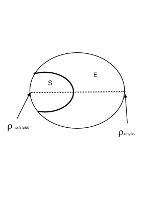
Figure 2: Set of asymptotic states for two qubits interacting with a common reservoir at infinite temperature. Here, $\rho_{mix~{}triplet}=\frac{1}{3}(\left|11\right\rangle\left\langle 11\right|+\left|\Psi_{+}\right\rangle\left\langle\Psi_{+}\right|+\left|00\right\rangle\left\langle 00\right|)$.

Since the singlet population remains fixed in the dynamics it allows us to identify the asymptotic state of any given initial condition. An initial state will have non-zero entanglement asymptotically if, and only if, $\rho_{44}>1/2$ so we have $P(AE)=P(D_{>1/2}=\{\rho\in D|\rho_{44}>1/2\})>0$. Of course $P(SBE)=P(D_{>1/2}\cap S)$. Since a state can exhibit ADE iff it relaxes to a state in the border between $S$ and $E$, we have $P(ADE^{\prime})\leq P(ADE)\leq P(ADE\cap\{\rho\in D|\rho_{44}=1/2\})=0$. So ADE is atypical for this dynamics but SDE, on the other hand, have a non-zero probability. In fact, an initially entangled state have SDE iff $\rho_{44}<1/2$, so $P(SDE^{\prime})=P(E\cap\{\rho\in D|\rho_{44}<1/2\})>0$.

All points belong to $\partial S$.

The combination of two reservoirs used in former examples will provide this case. If we have qubit $A$ subjected to spontaneous decay and $B$ to a phase reservoir the system will have the desired behavior, a situation that may occur experimentally if we entangle an atom in vacuum with a spin subjected to a stochastic magnetic field. That is, the system dynamics would be described by a master equation of the form (11a) (again in the interaction picture), but with $\mathcal{D}_{A}$ given by Eq. (7) (with $i=A$ and $\gamma_{A}^{\prime}=0$) and $\mathcal{D}_{B}$ by Eq. (11b) (with $i=B$). It is easy to see that the set of asymptotic states will be constituted by the product states where $A$ is in the $\left|0\right\rangle$ state and $B$ in a state described by a diagonal matrix (in the computational basis), so the global states reads:

$$\rho_{st}=\left(\begin{array}[]{cccc}0&0&0&0\\ 0&p&0&0\\ 0&0&0&0\\ 0&0&0&1-p\end{array}\right),$$ (25)

for $0\leq p\leq 1$. Whatever the value of $p$ we have Det$\rho_{st}$=Det$\rho_{st}^{\Gamma}=0$ so they indeed belong to $\partial S$. Again we have $SBE=AE=\emptyset$ for this dynamics, since there are no entangled asymptotic states, but to analise the probability of the other events we use the exact solution for the dynamics and write the determinant of the partial transpose in the form:

$$\text{Det}\rho(t)^{\Gamma}=f_{1}(\rho)e^{-\lambda_{1}t}+...+f_{n}(\rho)e^{-\lambda_{n}t},$$ (26)

where the functions $f_{i}$ depend on the initial state only, while $\lambda_{1}<\lambda_{2}<...<\lambda_{n}$. In this way, as long as $f_{1}\neq 0$, the asymptotic sign of Det$\rho(t)^{\Gamma}$ will by given by the sign of $f_{1}$. Denoting by $\gamma_{A}$ and $\gamma_{B}$ the decay rate for each reservoir, it so happens that $\lambda_{1}=2\gamma_{A}$ and $f_{1}=\text{Det}\rho^{\prime}$, where:

$$\rho^{\prime}=\left(\begin{array}[]{cccc}\rho_{11}&\rho_{12}^{*}&0&0\\ \rho_{12}&\rho_{11}+\rho_{22}&0&0\\ 0&0&\rho_{33}&\rho_{34^{*}}\\ 0&0&\rho_{34}&\rho_{33}+\rho_{44}\end{array}\right).$$ (31)

Since this matrix is positive definite (given that $\rho$ is), the system will reach its asymptotic state from the interior of the separables if $f_{1}(\rho^{\prime})>0$. But the event $f_{1}(\rho^{\prime})=0$ have zero probability, so we may conclude that $P(SDE)=P(SDE^{\prime})=P(E)$, while $P(ADE)=P(ADE^{\prime})=0$, that is, a sorted initial entangled state will exhibit sudden death of entanglement with certainty, in contrast with case 2a) where sudden and asymptotic death both had positive probabilities. Still, it is possible to find specific states where asymptotic death takes place. For instance, consider the set of initial states:

$$\rho=\left(\begin{array}[]{cccc}0&0&0&0\\ 0&\rho_{22}&\rho_{23}&0\\ 0&\rho_{23}^{*}&\rho_{33}&0\\ 0&0&0&0\end{array}\right).$$ (36)

The partial transpose determinant will be then Det$\rho(t)^{\Gamma}=-|\rho_{23}(t)|^{2}\rho_{22}(t)\rho_{33}(t)$, being negative for all $t$ if $\rho_{23},\rho_{22}$ and $\rho_{33}$ are initially different from zero, so the entanglement dies asymptotically.

Case 3a): One asymptotic state in $E$

The most natural way to realize a dynamics with this property is through a thermal reservoir. This time, though, interacting qubits and a common thermal reservoir are needed, that is, a reservoir that take any initial state to the Gibbs state $Z^{-1}\exp({-\beta H})$, with $Z=\text{Tr}\exp({-\beta H})$ and $H$ stands for the Hamiltonian describing the closed dynamics of the qubits. Typically, the ground state of interacting qubits Hamiltonian is non-degenerate and entangled, so if $\beta$ is large enough we obtain the desired dynamics.

Dynamics with these asymptotic states can be engineered using Lindblad autonomous equations, at least formally. Actually, fixed an arbitrary state for the system, there are many Linbdbladians that have this state as the only asymptotic state, in particular there are ones with only one Lindblad operator and null Hamiltonian part dietz . The specific Lindbladian of course, will depend on the specific interaction between qubits and reservoir (if the dynamics could be described by a Lindblad equation in the first place).

To give a more specific picture, consider, for instance, two interacting qubits described by the following Hamiltonian:

$$H=\frac{1}{2}\omega\sigma_{z,A}+\frac{1}{2}\omega\sigma_{z,B}+g(\sigma_{+,A}\sigma_{-,B}+\sigma_{-,A}\sigma_{+,B})$$ (37)

with $\omega,g$ positive constants satisfying $g>\omega$ (i.e., strong coupling limit). The eigenvalues for this Hamiltonian are, in crescent order, $-g,-\omega,\omega,g$, with respective eigenvectors $\left|\Psi_{-}\right\rangle,\left|00\right\rangle,\left|11\right\rangle,\left|\Psi_{+}\right\rangle$, leading to an entangled ground state. Denote by $\left|i\right\rangle$, $i=1,\ldots,4$ these eigenvectors according to their eigenvalues order. We may consider a thermal reservoir at null temperature that induces decays between any two of these states in a Markovian way, such that the dissipator would be:

$$\mathcal{D}[\rho]=\sum_{i<j}\gamma_{ij}(2\sigma_{ij}\rho\sigma_{ji}-\sigma_{jj}\rho-\rho\sigma_{jj}),$$ (38)

where $\sigma_{ij}=\left|i\right\rangle\left\langle j\right|$ and $\gamma_{ij}$ are non-negative constants. A dissipator of this type can be derived from a microscopic model, for instance, adapting the results of Ref. scala to the Hamiltonian considered here .

As in case 1a), the events and probabilities we are interested in are trivial: $SBE=S,AE=D$, i.e., every initial state will acquire entanglement for large times, in particular the separable ones, so $P(SBE)=P(S)$ and $P(AE)=1$. Since the entanglement never vanishes, $ADE=ADE^{\prime}=SDE=SDE^{\prime}=\emptyset$

Case 3b): Several asymptotic states in $E$

Examples for this case can be provided just by the same trick used in case 1b): we take any Lindbladian with only one asymptotic entangled state and insert a time varying coupling which multiplies the dissipator. The same reasoning can be applied with respect to the asymptotic states for the subsequent dynamics (in the interaction picture), so, if the decay rate of the coupling is small enough, the set of asymptotic states will be constituted by a small “blurring” around the asymptotic state of the dynamics with constant coupling.

Contrary to case 1b), though, in what entanglement is concerned, it is important now whether the dynamics is given in the Schrödinger or interaction pictures, because their correspondence is given by global unitary transformations. By the same reason as before, the dynamics will not be relaxing in the Schrödinger picture, but one can still find a non-trivial asymptotic set, this time, entirely contained in $E$. Indeed, diminishing the decay rate of the reservoir couplings, we can diminish at will the diameter of the set of stationary states in the interaction picture which, by its turn, always contain the Gibbs state of the system. Now, unitary transformations are isometries for practically all relevant metrics, so the set of asymptotic states in the interaction picture is mapped to sets with the same diameter in the Schrödinger picture. But these unitary transformations have the Gibbs state as a fixed point, hence these sets always contains it. Since $E$ is open, given that their diameter is small enough, we can be sure that they always fall entirely inside of it.

As a consequence of the discussion in the above paragraph, the events and probabilities we are considering in this paper are identical to the ones in the last example.

IV Conclusions

In this paper we review the classification of the possible dynamics of entanglement based on the relative geometry of the sets of asymptotic and separable states. We provided examples for all possible classes, including the previously unknown cases with more than one asymptotic state, but avoiding the boundary $\partial S$. In giving those examples it was sufficient to use two-qubit dynamics dictated by equations of motion in Lindblad form (including non-autonomous dynamics exactly for those previously hard examples). In each case, the existence of sudden death of entanglement, asymptotic death of entanglement, sudden birth of entanglement and asymptotic entanglement were analyzed from a more precise point of view, looking at the probabilities that each of these phenomena occur if one choose a random initial state and a suitable probability measure on the set of quantum states.

- (1) E. Schr dinger, Proceedings of the Cambridge Philosophical Society 31, 555 (1935).
- (2) C. H. Bennett, G. Brassard, C. Crépeau, R. Jozsa, A. Peres, W. K. Wootters, Phys. Rev. Lett. 70, 1895 (1993).
- (3) M. Nielsen and I. Chuang, Quantum Computation and Quantum Information (Cambridge University Press, Cambridge, UK, 2000).
- (4) A. K. Ekert, Phys. Rev. Lett. 67, 661 (1991). Although most schemes of quantum cryptography do not explicitly uses entangled states, entanglement is important to prove their security renner .
- (5) R. Renner, Ph.D. Thesis (2005); arXiv:quant-ph/0512258.
- (6) V. Vedral, M.B. Plenio, M.A. Rippin, and P.L. Knight, Phys. Rev. Lett. 78, 2275 (1997).
- (7) M. Koashi and A. Winter Phys. Rev. A 69, 022309 (2004).
- (8) K. Życzkowski, P. Horodecki, M. Horodecki, and R. Horodecki, Phys. Rev. A65, 012101 (2001); T. Yu and J. H. Eberly, Phys. Rev. B66, 193306 (2002); L. Diósi, Lect. Notes Phys. 622, 157 (2003); P. J. Dodd and J. J. Halliwell, Phys. Rev. A69, 052105 (2004).
- (9) T. Yu and J. H. Eberly, Opt. Commun. 264, 393 (2006).
- (10) F. Lastra, G. Romero, C. E. López, M. França Santos, and J. C. Retamal, Phys. Rev. A 75, 062324 (2007); K. Ann and G. Jaeger Phys. Rev. B75, 115307 (2007); L. Aolita, R. Chaves, D. Cavalcanti, A. Acín, and L. Davidovich Phys. Rev. Lett. 100, 080501 (2008).
- (11) M. F. Santos, P. Milman, L. Davidovich, and N. Zagury, Phys. Rev. A 73, 040305(R) (2006).
- (12) M. P. Almeida, F. de Melo, M. Hor-Meyll, A. Salles, S. P. Walborn, P. H. Souto Ribeiro, and L. Davidovich, Science 316, 579 (2007).
- (13) M. O. Terra Cunha, New J. Phys. 9 237 (2007).
- (14) S. L. Braunstein, C.M. Caves, R. Jozsa, N. Linden, S. Popescu, and R. Schack Phys. Rev. Lett. 83, 1054 (1999).
- (15) C. Viviescas, private communication.
- (16) P. B. Slater, J. Geom. Phys. 53 74 (2005).
- (17) K. Życzkowski, I. Bengtsson, Geometry of Quantum States: An Introduction to Quantum Entanglement (Cambridge University Press, Cambridge, UK, 2006).
- (18) G. Lindblad, Commun. Math. Phys. 48, 119 (1976).
- (19) F. Verstraete, K. Audenaert, J. Dehaene and B. De Moor J. Phys. A: Math. Gen. 34 (2001).
- (20) R. F. Werner, Phys. Rev. A 40, 4277 (1989).
- (21) M.O. Terra Cunha and M.C. Nemes, Phys. Lett. A 329, 409 (2004).
- (22) S. Schneider and G. J. Milburn Phys. Rev A 65, 042107 (2002).
- (23) K. Dietz, J. Phys. A: Math. Gen. 37, 6143 (2004).
- (24) M. Scala, R. Migliore, A. Messina, arXiv:0806.4852v1 [quant-ph].