Ground-state properties of the two-site Hubbard-Holstein model: an exact solution

Abstract

We revisit the two-site Hubbard-Holstein model by using extended phonon coherent states. The nontrivial singlet bipolaron is studied exactly in the whole coupling regime. The ground-state (GS) energy and the double occupancy probability are calculated. The linear entropy is exploited successfully to quantify bipartite entanglement between electrons and their environment phonons, displaying a maximum entanglement of the singlet-bipolaron in strong coupling regime. A dramatic drop in the crossover regime is observed in the GS fidelity and its susceptibility. The bipolaron properties is also characterized classically by correlation functions. It is found that the crossover from a two-site to single-site bipolaron is more abrupt and shifts to a larger electron-phonon coupling strength as electron-electron Coulomb repulsion increases.

I introduction

It has been demonstrated for more than one decade that the polaronic effects observed in High-$T_{c}$ superconducting cuprates ASAlexandrov and the colossal magnorestive manganites AJMilis are relevant to the electron-phonon (e-ph) coupling in these systems. The famous Holstein molecular crystal model THolstein , where electrons are coupled with local phonons, has then revived in recent years. More recently, to include the electron-electron (e-e) Coulomb repulsion interactions, the Hubbard-Holstein (HH) model Fehske for strongly correlated electron systems has made significant progress in understanding many-body aspects. As is well known, an exact solution to this model in the thermodynamic limit is impossible, and many approximate approaches are then employed. The two-site HH model, where two electrons hop between two adjacent lattice sites, can be solved analyticallyBerciu . It is not only a prototype of the HH model but also helpful for the better understanding to the polaron and bipolaron behavior in infinite lattices.

Recently, an contemporary alternative characterization of the ground state (GS) properties has been focused on quantum information tools in terms of quantum entanglement Scott ; William ; Vidal ; Gu ; chenqh and fidelity Quan ; Zanardi ; Vezzani ; Min ; Shu ; Buon ; Chen . These studies will establish somewhat interesting understanding from the field of quantum information theory to condensed matter physics Dunning ; Norman . Usually, it is hard to calculate these quantities due to the lack of knowledge on the exact GS wave function.

The two-site HH model has been previously addressed by means of different methods, such as variational method ANDas ; Acquarone , perturbation theory JC , and numerical diagonalizationRanninger ; EVLde . In spite of these efforts there remains poor convergence in the intermediate coupling regime. A reliable treatment in the whole coupling regime is still needed. Recently, Berciu derived all Greens’s function analytically for the two-site HH model in terms continued fractionsBerciu .

In this work, by using extended bosonic coherent states  chen ; Han ; liu , we develop a new exact technique to deal with the two-site HH model. The wave function is proposed explicitly, by which many quantities can be calculated directly. The paper is organized as follows. In Sec II we introduce the model and describe the approach. In Sec III we calculate the linear entropy , the GS fidelity and its susceptibility to study crossover properties from quantum information perspective. The static correlation function is also evaluated to analyze the GS properties. The main conclusions are given in the last section.

II Model Hamiltonian and exact solution

The Hamiltonian of the two-site HH model takes the form

$$H = \sum_{i,\sigma}\varepsilon n_{i\sigma}-\sum_{\sigma}t(c_{1\sigma}^{\dagger}c_{2\sigma}+c_{2\sigma}^{\dagger}c_{1\sigma})$$ (1)

$$+ U\sum_{i}n_{i\uparrow}n_{i\downarrow}+Vn_{1}n_{2}+g_{1}\omega_{0}\sum_{i,\sigma}n_{i,\sigma}(b_{i}+b_{i}^{\dagger})$$

$$+ g_{2}\omega_{0}\sum_{i,\sigma}n_{i,\sigma}(b_{i+\delta}+b_{i+\delta}^{\dagger})+\omega_{0}\sum_{i}b_{i}^{\dagger}b_{i},$$

where $i(=1$ or $2$) denotes the label of sites. $i+\delta=2$ for $i=1$ and vice versa. $c_{i\sigma}(c_{i\sigma}^{\dagger})$ is the annihilation (creation) operator for the electrons and $n_{i,\sigma}(=c_{i\sigma}^{\dagger}c_{i\sigma})$ is the corresponding number operator at site $i$ with spin $\sigma$, besides $n_{i}=n_{i\uparrow}+n_{i\downarrow}$. $\varepsilon$ is the unperturbed site potential. $t$ is the usual hopping integral. $U$ and $V$ denote the on-site and inter-site Coulomb repulsion between electrons respectively. $g_{1}$ and $g_{2}$ denote the on-site and inter-site e-ph coupling parameters. $b_{i}(b_{i}^{\dagger})$ is the annihilation (creation) operator for phonons corresponding to interatomic vibrations at site $i$. $\omega_{0}$ is the phonon frequency and is set unit for convenience in the following.

Introducing new phonon operators $a=(b_{1}+b_{2})/\sqrt{2}$ and $d=(b_{1}-b_{2})/\sqrt{2}$, the Hamiltonian  (1) can be written into two independent parts ($H=H_{d}+H_{a}$),

$$H_{d} = d^{\dagger}d+\sum_{i,\sigma}\varepsilon n_{i\sigma}-\sum_{\sigma}t(c_{1\sigma}^{\dagger}c_{2\sigma}+c_{2\sigma}^{\dagger}c_{1\sigma})$$ (2)

$$+ U\sum_{i}n_{i\uparrow}n_{i\downarrow}+Vn_{1}n_{2}$$

$$+ g_{-}(n_{1}-n_{2})(d+d^{\dagger})-n^{2}g_{+}^{2}$$

and

$$H_{a}=\tilde{a}^{\dagger}\tilde{a},$$ (3)

where $\tilde{a}^{\dagger}=a^{\dagger}+ng_{+}$, $\tilde{a}=a+ng_{+}$, $g_{+}=(g_{1}+g_{2})/\sqrt{2}$, and $g_{-}=(g_{1}-g_{2})/\sqrt{2}$. $H_{a}$ describes a shifted oscillator and represents lowering of energy, which is a constant motion. $H_{d}$ represents an effective e-ph coupling system which phonons are coupled linearly with the electrons.

In the effective Hamiltonian $H_{d}$, among four different bipolaronic states, such as singlet bipolaronic states, singlet Anderson bipolaronic states, singlet bipolaronic states (antibonding), and triplet states, the singlet bipolaronic state is the most nontrivial to any approaches. We will focus on this state in this paper.

For three singlet normalized electronic states $c_{1\uparrow}^{\dagger}c_{1\downarrow}^{\dagger}|0\rangle_{e}$, $c_{2\uparrow}^{\dagger}c_{2\downarrow}^{\dagger}|0\rangle_{e}$ and $\frac{1}{\sqrt{2}}(c_{1\uparrow}^{\dagger}c_{2\downarrow}^{\dagger}-c_{1\downarrow}^{\dagger}c_{2\uparrow}^{\dagger})|0\rangle_{e}$, the singlet bipolaronic state wave function $|\psi\rangle$ can be expressed as

$$|\psi\rangle = |\varphi_{1}\rangle c_{1\uparrow}^{\dagger}c_{1\downarrow}^{\dagger}|0\rangle_{e}+|\varphi_{2}\rangle c_{2\uparrow}^{\dagger}c_{2\downarrow}^{\dagger}|0\rangle_{e}$$ (4)

$$+ |\varphi_{3}\rangle\frac{1}{\sqrt{2}}(c_{1\uparrow}^{\dagger}c_{2\downarrow}^{\dagger}-c_{1\downarrow}^{\dagger}c_{2\uparrow}^{\dagger})|0\rangle_{e}$$

where $|\varphi_{1}\rangle$, $|\varphi_{2}\rangle$ and $|\varphi_{3}\rangle$ correspond to phonon states. Inserting it into a schrödinger equation for the effective Hamiltonian in Eq. (2), three equations are derived by comparing the coefficients of $c_{1\uparrow}^{\dagger}c_{1\downarrow}^{\dagger}|0\rangle_{e}$, $c_{2\uparrow}^{\dagger}c_{2\downarrow}^{\dagger}|0\rangle_{e}$ and $\frac{1}{\sqrt{2}}(c_{1\uparrow}^{\dagger}c_{2\downarrow}^{\dagger}-c_{1\downarrow}^{\dagger}c_{2\uparrow}^{\dagger})|0\rangle_{e}$,

$$[A^{\dagger}A+2\varepsilon-4(g_{1}^{2}+g_{2}^{2})+U]|\varphi_{1}\rangle-\sqrt{2}t|\varphi_{3}\rangle=E|\varphi_{1}\rangle$$ (5)

$$[B^{\dagger}B+2\varepsilon-4(g_{1}^{2}+g_{2}^{2})+U]|\varphi_{2}\rangle-\sqrt{2}t|\varphi_{3}\rangle=E|\varphi_{2}\rangle$$ (6)

$$[d^{\dagger}d+2\varepsilon-2(g_{1}+g_{2})^{2}+V]|\varphi_{3}\rangle-\sqrt{2}t(|\varphi_{1}\rangle+|\varphi_{2}\rangle)=E|\varphi_{3}\rangle$$ (7)

where we have used two displacement transformation $A^{\dagger}=d^{\dagger}+2g_{-}$ and $B^{\dagger}=d^{\dagger}-2g_{-}$. Note that the linear term for the phonon operator $d(d^{+})$ is removed, and two new free bosonic field with operator $A(A^{+})$ and $B(B^{+})$ appear. In the next step, we naturally choose the basis in terms of these new operator, instead of $d(d^{+})$, by which the phonon states $|\varphi_{1}\rangle$ and $|\varphi_{2}\rangle$ can be expanded in complete basis ${|n\rangle_{A}}$ and ${|n\rangle_{B}}$ respectively, where $|n\rangle_{A}$ and $|n\rangle_{B}$ are Fock states of the new bosonic operators

$$|\varphi_{1}\rangle =\sum_{n=0}^{N_{tr}}c_{n}|n\rangle_{A}$$ (8)

$$= \sum_{n=0}^{N_{tr}}c_{n}\frac{1}{\sqrt{n!}}(d^{\dagger}+2g_{-})^{n}e^{-2g_{-}d^{\dagger}-2g_{-}^{2}}|0\rangle_{ph}$$

$$|\varphi_{2}\rangle =\sum_{n=0}^{N_{tr}}d_{n}|n\rangle_{B}$$ (9)

$$= \sum_{n=0}^{N_{tr}}d_{n}\frac{1}{\sqrt{n!}}(d^{\dagger}-2g_{-})^{n}e^{2g_{-}d^{\dagger}-2g_{-}^{2}}|0\rangle_{ph}$$

As we know that the vacuum state $\left|0\right\rangle_{A(B)}$ is just a bosonic coherent-state in $d(d^{+})$ with an eigenvalue $2g(-2g_{-})$chen ; Han ; liu . So this new basis is overcomplete, and actually does not involve any truncation in the Fock space of $d(d^{+})$, which highlights the present approach. It is also clear that many-body correlations for bosons are essentially included in extended coherent states (8) and (9). As usual, the phonon state $|\varphi_{3}\rangle$ is expanded in a complete basis ${|n\rangle}$, which is the Fock state of $d(d^{+})$

$$|\varphi_{3}\rangle=\sum_{n=0}^{N_{tr}}f_{n}|n\rangle$$ (10)

Substituting these phonon states (8), (9), and (10) into Eqs. (5),( 6) and  (7) and left multiplying state ${}_{A}\langle m|$, ${}_{B}\langle m|$, $\langle m|$, respectively, the equations can be written as $3N_{tr}\times 3N_{tr}$ matrix, and the $m^{\prime}$th row is written as

$$[m+2\varepsilon-4(g_{1}^{2}+g_{2}^{2})+U]c_{m}-\sqrt{2}t\sum_{n}{{}_{A}\langle m}|n\rangle f_{n}=Ec_{m}$$ (11)

$$[m+2\varepsilon-4(g_{1}^{2}+g_{2}^{2})+U]d_{m}-\sqrt{2}t\sum_{n}{{}_{B}\langle m}|n\rangle f_{n}=Ed_{m}$$ (12)

$$[m +2\varepsilon-2(g_{1}+g_{2})^{2}+V]f_{m}-\sqrt{2}t(\sum_{n}c_{n}\langle m|n\rangle_{A}$$ (13)

$$+ \sum_{n}d_{n}\langle m|n\rangle_{B})=Ef_{m}$$

where ${}_{A}\langle m|n\rangle=\langle m|n\rangle_{B}=(-1)^{n}D_{mn}$, and ${}_{B}\langle m|n\rangle=\langle m|n\rangle_{A}=(-1)^{m}D_{mn}$, with $D_{mn}=e^{-2g_{-}^{2}}\sum_{i=0}^{{min}[m,n]}(-1)^{-i}\frac{\sqrt{m!n!}(2g_{-})^{m+n-2i}}{(m-i)!(n-i)!i!}$.

The eigenvalues $E$ and eigenvectors with coefficients ${c_{n}}$, ${d_{n}}$ and $f_{n}$ can be exactly solved by diagonalizing the above $3N_{tr}\times 3N_{tr}$ matrix numerically.

To obtain the true exact results, in principle, the truncated number $N_{tr}$ should be taken to infinity. Fortunately, finite terms of the singlet state in Eq.(4) are sufficient to give very accurate results in the whole parameter range. It should be noted that in the exact diagonalization in Fock space of original phonon state $d$ EVLde , a considerable large phonon number is needed to give reasonably good results. We believe that we have exactly solved this model numerically.

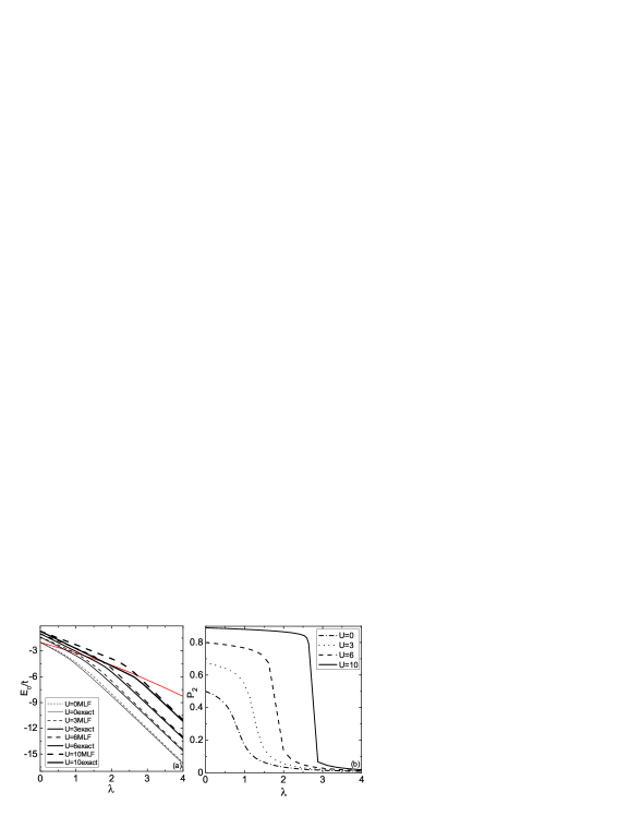
Figure 1: (a) GS energy $E_{0}/t$ of exact solution (solid line) and MLFS transformation (dashed line) vs $\lambda$ for $U=0,3,6$ and $10$. The red line represents the twice polaron GS energy, which then separates the polaron and bipolaron regime. (b) The probability of the two-site bipolarons $P_{2}$ for $U=0$, $3$, $6$, and $10$. The other parameters are chosen: $V=0$, $t=2.0$, $\varepsilon=0$.

To show the effectiveness of the present approach, we first calculate the GS energy. Fig. 1(a) presents the GS energy $E_{0}/t$ as a function of the on-site effective coupling strength $\lambda=g_{1}^{2}/t$ by setting $g_{2}=0$ conveniently. The results for the energy by the variational method based on the modified Lang-Firsov transformation with a squeezing phonon state transformations (MLFS) ANDas are also list. It is observed that the present results are lower than the MLFS results ANDas , especially in the intermediate coupling regime. Comparing with the Fig. 1(a) in Ref. Berciu , we find that the present results for the GS energy are consistent with those from the lowest pole of a Green’s function.

III ground state properties

III.1 Crossover from two-site to single-site bipolarons

As shown in Fig. 1(a) that there is two regimes distinctly. In the Ref. Berciu , the energy vs $\lambda$ curves in two regimes are fitted by two functions, and the abrupt drop of the first-order derivative signals the crossover regime from two-site bipolarons to single-site bipolarons. We will propose a quantitative criterion. Because the exact wave function in the present technique is explicitly given, we can calculate the probability of the system that two electrons are in two sites by Eq. (4) directly.

$$P_{2}=Re\langle\varphi_{3}|\varphi_{3}\rangle$$ (14)

The probability of the two-site bipolarons $P_{2}$ is shown in Fig. 1(b). At the weak coupling, the two electrons prefer to stay in two sites. As the coupling strength increases, the two electrons tend to occupy the single site. Strictly speaking, at weak (strong) coupling, it is not pure two-site (single-site) bipolarons, only dominated two-site (single-site) bipolarons. The crossover regime is wide for weak on-site Coulomb repulsion $U$. As $U$ increases, the crossover shifts to larger $\lambda$ and becomes more sharp. However, the jump of the $P_{2}$ is not observed, indicating unlikely a phase transition.

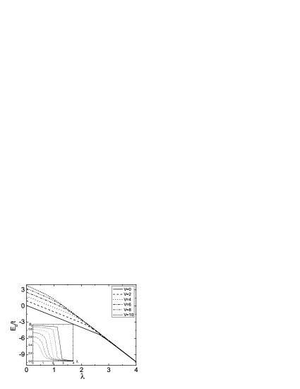
Figure 2: GS energy $E_{0}/t$ and the probability of the two-site bipolarons $P_{2}$ in the inset vs $\lambda$ for $V=0,2,4,6,8,10$ by choosing $V=0.2$, $t=2.0$, $\varepsilon=0.8$.

The inter-site Coulomb repulsion $V$ may favor the formation of dominated single-site bipoalrons. To show this effect, we calculate the GS energy and the probability of the two-site bipolarons for several values of $V$ for fixed $U$, which are displayed in Fig. 2. It is clear that the crossover shifts to smaller $\lambda$ with increasing $V$, and becomes more smooth.

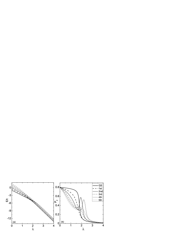
Figure 3: GS energy and the former five excited energies $E/t$ (a) and the corresponding probability $P_{2}$ (b) against $\lambda$ for $U=6$ by choosing $V=0.2$, $t=2.0$, $\varepsilon=0.8$.

In our approach, we can also get the excited states and corresponding energies. Both the GS and a few low excited state bipolaron energies for $U=6$ are presented in Fig. 3(a). Interesting, we find that the curves for the GS and the 1st excited state energies, the 2nd and 3rd excited state energies, 4th and 5th excited state energies almost merge into a single line in the strong coupling regime. The corresponding two eigenstates are almost degenerated. Actually they are different. The difference is too small to be observed. The merged point shift to larger $\lambda$ for higher excited states. To show the bipolaron behavior in these states, we also calculate the probability of the two-site bipolarons $P_{2}$ as a function of $\lambda$, which are shown in Fig.3(b). The $P_{2}$ vs $\lambda$ curves also merge into a single line exactly at the same point as the energy vs $\lambda$ curves. In the GS and 1st excited state, the value of $P_{2}$ decreases monotonously as $\lambda$. However, in the other high excited states, a non-monotonous behavior of the $P_{2}$ is observed. In a fixed value of $\lambda$, the probability of the two-site bipolarons $P_{2}$ determines the positive repulsion energy for the double occupancy, the energy gained for the two electrons in the same site, and the energy gained for the hopping of electrons from one site to other site. To increase the energy in higher excited states, the competition of these energies contributes the complicated behavior shown in Fig.3(b).

III.2 Linear entropy

To investigate the crossover from two-site to single-site bipolarons in quantum information science, we attempt to study quantum entanglement between electrons and their surrounding phonons by means of the linear entropy $E_{l}$ Yang ; Wang , which is an alternative measurement to indicate the entanglement of a two-site and single-site bipolaron. It is defined as

$$E_{l}=1-{Tr}\rho^{2},$$ (15)

where $\rho=Tr_{ph}(|\psi\rangle\langle\psi|)$ is the reduced density matrix of electrons by taking partial trace over the phonon degrees of the freedom.

The normalized GS wave function of the singlet bipolaronic state in Eq.(4) is described as

$$|\psi\rangle=|\varphi_{1}\rangle|1\rangle+|\varphi_{2}\rangle|2\rangle+|\varphi_{3}\rangle|3\rangle,$$ (16)

where the phonon states satisfy $\langle\varphi_{1}|\varphi_{1}\rangle+\langle\varphi_{2}|\varphi_{2}\rangle+\langle\varphi_{3}|\varphi_{3}\rangle=1$. And the quantum states $|1\rangle$, $|2\rangle$ and $|3\rangle$ represent the normalized and orthogonalized singlet electronic states $c_{1\uparrow}^{\dagger}c_{1\downarrow}^{\dagger}|0\rangle_{e}$ $c_{2\uparrow}^{\dagger}c_{2\downarrow}^{\dagger}|0\rangle_{e}$ and $\frac{1}{\sqrt{2}}(c_{1\uparrow}^{\dagger}c_{2\downarrow}^{\dagger}-c_{1\downarrow}^{\dagger}c_{2\uparrow}^{\dagger})|0\rangle_{e}$ respectively.

The reduced density matrix $\rho$ can be derived by taking partial trace over the phonon degrees of the freedom $\rho=\sum^{3}_{i,j=1}{\langle\varphi_{j}}|\varphi_{i}\rangle|i\rangle\langle j|$. Therefore the linear entropy can be derived simply as

$$E_{l} = 1-[\langle\varphi_{1}|\varphi_{1}\rangle^{2}+\langle\varphi_{2}|\varphi_{2}\rangle^{2}+\langle\varphi_{3}|\varphi_{3}\rangle^{2}$$ (17)

$$+ 2Re(\langle\varphi_{1}|\varphi_{2}\rangle^{2}+\langle\varphi_{1}|\varphi_{3}\rangle^{2}+\langle\varphi_{2}|\varphi_{3}\rangle^{2})]$$

As plotted in Fig.4, the linear entropy $E_{l}$ increases smoothly with the e-ph coupling parameters $\lambda$ for different e-e Coulomb repulsions $U$. In general, in weak e-ph coupling region, two electrons tend to occupy two sites, and form so-called two-site bipolaron, resulting a low degree of the quantum entanglement in the original coupling strength. For a fixed $U$, as $\lambda$ increases two electrons become to tightly interact with the same lattice. So the entire charge of the electrons and entire deformations of the lattices are restricted on one site, leading to the formation of a single-site bipolaron. However, the two-site bipolaron is known as that each electron just interacts with phonons of its own site and then the linear entropy is expected to be much smaller than that of the singlet-site bipolaron. As shown in Fig.4 the linear entropy reaches its maximum $E_{l}=0.5$ in the strong coupling region, which displays that the single-site bipolarons are maximally entangled. Obviously the crossover point shifts to a large value of the coupling strength $\lambda$ as $U$ increases. The similar crossover point has been demonstrated by the probability of the two-site bipolarons presented in Fig. 1(b). Therefore we can say that in the presence of quantum correlations the two-site and singlet-site bipolarons are effectively characterized to a high (low) degree of bipartite quantum entanglement.

Figure 4: Linear entropy $E_{l}$ vs $\lambda$ for $U=0,3,6,10$ by choosing $V=0.2$, $t=2.0$, $\varepsilon=0.8$. The maximum $E_{l}=0.5$ corresponds to the single-site bipolaron in strong coupling region.

III.3 ground state fidelity

More recently, another temporary effective quantum information tools, i.e., the fidelity has been put forward to analyze complicated interacting systems from the perspective of the GS wave functions Shu ; Chen , first identifying polaronic crossover behaviors in bosonic system Norman . A simple expression of the fidelity $F(g_{1},g_{1}+\delta g_{1})$ is given just by the modulus of the overlap of two ground states corresponding to two different coupling parameters $g_{1}$ and $g_{1}+\delta g_{1}$, where $g_{1}$ is a tiny perturbation parameter Zanardi . It is expected to signal a peak at the critical point. The general GS fidelity is written as

$$F = \langle\psi(g_{1})|\psi(g_{1}+\delta g_{1})\rangle$$ (18)

$$= |\langle\varphi_{1}(g_{1})|\varphi_{1}(g_{1}+\delta g_{1})\rangle+\langle\varphi_{2}(g_{1})|\varphi_{2}(g_{1}+\delta g_{1})\rangle$$

$$+ \langle\varphi_{3}(g_{1})|\varphi_{3}(g_{1}+\delta g_{1})\rangle|$$

where $|\psi(g_{1})\rangle$ and $|\psi(g_{1}+\delta g_{1})\rangle$ are two normalized GS corresponding to neighboring Hamiltonian parameters. In our calculation $\delta g_{1}=10^{-4}$ is used. While the fidelity susceptibility $S(g_{1})$ is regarded as a more effective tool to detect the singularity at the crossover regime, which reads Cozzini

$$S(g_{1})=\lim_{\delta g_{1}\longrightarrow 0}[1-F(g_{1},g_{1}+\delta g_{1})]/(\delta g_{1}^{2})$$ (19)

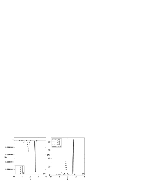
Figure 5: GS fidelity $F$ and its susceptibility $S$ versus $\lambda$ for $U=0,3,6,10$ by choosing $V=0.2$, $t=2.0$, $\varepsilon=0.8$. A sharper drop is shown at the crossover for larger $U=10$(solid line).

The GS fidelity $F$ and its susceptibility $S$ as a functions of effective coupling strength $\lambda$ ($=g_{1}^{2}/t$) for different e-e Coulomb repulsion $U$ are displayed in Fig. 5(a) and (b). A narrow dramatic drop is observed in the vicinity of the bipolaron transition point as a consequence of the dramatic change of the structure of the GS wave function, implying that the crossover from the two-site to singlet-site bipolaron occurs. As shown in Fig. 5(a), the values of the GS fidelity are approximated to $1$. As is known, for the quantum phase transition system the GS wave functions from different sides of the level-crossing point are almost orthogonal Shu . However, there is absent of the level-crossing and then values of peaks of the GS fidelity are around to $1$ rather than $0$ at the crossover point. Further evidence for this crossover is given by the susceptibility $S$, which shows a cusp structure in the intermediate coupling regime in Fig. 5(b). Obviously, the crossover becomes more abrupt and the critical value of the e-ph coupling $\lambda$ where the peak appears becomes larger as the Coulomb repulsion $U$ increases from $0$ to $10$. So it is illustrated that the transition behavior from two-site to singlet-site bipolaron can be effectively detected by a singularity of the GS fidelity and its susceptibility.

III.4 static correlation function

Since the bipolaron crossover transition has been indeed known from the quantum information perspective. Naturally, we seek classically to discuss this crossover by the means of the static on-site and inter-site correlation functions $\langle n_{1}u_{1}\rangle$ and $\langle n_{1}u_{2}\rangle$, which reveal the spatial extent of lattice deformations induced by electrons respectively. The $u_{i}$ denotes the lattice deformations on site $i$ produced by the electrons and $n_{i}$ is the number operator of the electrons. The GS correlation functions are written as

$$\langle n_{1}u_{1,2}\rangle=\langle n_{1}[\pm(d+d^{\dagger})/2-2gn_{1,2}]\rangle$$ (20)

The positive (negative) sign and $n_{1}$ ($n_{2}$) are associated with $\langle n_{1}u_{1}\rangle$ and $\langle n_{1}u_{2}\rangle$ respectively. By using the exact GS wave function of the singlet bipolaronic state obtained above, the correlation functions Eq.(20) can be expressed as follows

$$\langle n_{1}u_{2}\rangle=-2g_{1}\sum_{m=0}^{N}f_{m}^{2}-$$

$$\sum_{m=1}^{N}\sqrt{m}(c_{m}^{*}c_{m-1}+0.5f_{m}^{*}f_{m-1})$$

$$-\sum_{m=0}^{N-1}\sqrt{m+1}(c_{m}^{*}c_{m+1}+0.5f_{m}^{*}f_{m+1})$$ (21)

$$\langle n_{1}u_{1}\rangle = -2g_{1}\sum_{m=0}^{N}(4c_{m}^{2}+f_{m}^{2})$$ (22)

$$+\sum_{m=1}^{N}\sqrt{m}(c_{m}^{*}c_{m-1}+0.5f_{m}^{*}f_{m-1})$$

$$+\sum_{m=0}^{N-1}\sqrt{m+1}(c_{m}^{*}c_{m+1}+0.5f_{m}^{*}f_{m+1}).$$

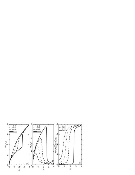
Figure 6: Correlation function versus $\lambda$ (a)$-\langle n_{1}u_{1}\rangle$, (b)$-\langle n_{1}u_{2}\rangle$, (c)$-\langle(n_{1}-n_{2})(u_{1}-u_{2})\rangle/g_{1}$ for $U=0,3,6,10$ by choosing $V=0.2$, $t=2.0$, $\varepsilon=0.8$. A more abrupt crossover occurs for larger $U=10$ (solid line).

The functions $-\langle n_{1}u_{1}\rangle$ and $-\langle n_{1}u_{2}\rangle$ against the e-ph coupling strength $\lambda$ are plotted in Figs. 6 (a) and (b). One can observe that $-\langle n_{1}u_{1}\rangle$ and $-\langle n_{1}u_{2}\rangle$ increase monotonically with $\lambda$ in weak coupling regime. When $\lambda$ exceeds a critical value, $-\langle n_{1}u_{1}\rangle$ and $-\langle n_{1}u_{2}\rangle$ show different behaviors. It is clearly shown that two electrons are localized on one site in strong coupling region, resulting the singlet-site bipolaron. It also demonstrates that the e-e interaction $U$ affects the magnitude of inter-site (on-site) deformations $\langle n_{1}u_{2}\rangle$ ($-\langle n_{1}u_{1}\rangle$) and the transition point where $-\langle n_{1}u_{2}\rangle$ reaches maximum shifts to a larger $\lambda$ as $U$ increases.

The nature of the bipolaron crossover can also be investigated by the correlation function $\langle(n_{1}-n_{2})(u_{1}-u_{2})\rangle/g_{1}$. Figs.6(c) shows that the two-site bipolaron regime of the coupling strength $\lambda$ is wider for larger $U$ in the weak e-ph coupling regime. This crossover behaviors are consistent with the above analysis on the GS entanglement and fidelity.

IV summary and discussion

In this present work we have solved exactly the two-site Hubbard-Holstein model by the extended phonon coherent states approach. The GS energy is lower than previous results and the crossover regime is revealed clearly by the electrons occupancy probability. With the exact GS wave function, we study the crossover properties from quantum information perspective based on the linear entropy, the GS fidelity and its susceptibility. The single-site bipolarons are maximally entangled and the bipolaron crossover transition is more abrupt as e-e interaction $U$ increases. The similar bipolaron crossover behaviors are also observed classically in the static correlation function. The present study may provide some insights into the more complicated Hubbard-Holstein systems in a infinite chain.

V Acknowledgements

This work was supported by National Natural Science Foundation of China, PCSIRT (Grant No. IRT0754) in University in China, National Basic Research Program of China (Grant No. 2009CB929104).

^†Corresponding author

References

- (1) A. S. Alexandrov, and N. F. Mott, polarons and Bipolarons, World Scientific, Singapore (1995); A. Damascelli, Z. Hussain, and Z. X. Shen, Rev. Mod. Phy. 75, 473 (2003).
- (2) A. J. Millis, Nature (London) 392,147(1998); D. M. Edwards, Adv. Phys. 51, 1259 (2003).
- (3) T. Holstein, Ann. Phy. (NY) 8, 325 (1959).
- (4) H. Fehske, G. Wellein, J. Loos, and A. R. Bishop, Phys. Rev. B 77 , 085117 (2008).
- (5) M. Berciu, Phys. Rev. B 75, 081101(R) (2007).
- (6) S. Hill, and W. K. Wootters, Phys. Rev. Lett. 78, 26 (1997).
- (7) W. K. Wootters, Phys. Rev. Lett. 80, 10 (1998).
- (8) G. Vidal, J. I. Latorre, E.Rico, and A.Kitaev, Phys. Rev. Lett. 90, 227902 (2003).
- (9) S. J. Gu, S. S. Deng, Y. Q. Li, and H. Q. Lin, Phys. Rev. Lett. 93, 086402 (2004).
- (10) Q. H. Chen, Y. Y. Zhang, T. Liu, and K. L. Wang, Phys. Rev. A (in press); see also arXiv: 0809.4385.
- (11) H. T. Quan, Z. Song, X. F. Liu, P. Zanardi, and C. P. Sun, Phys. Rev. Lett. 96, 140604 (2006).
- (12) P. Buonsante, and A. Vezzani, Phys. Rev. Lett. 98, 110601 (2007).
- (13) M. F. Yang, arxiv:quant-ph/07074574
- (14) S. Chen, L. Wang, Y. J. Hao, and Y. P. Wang, Phys. Rev. A. 77, 032111 (2008) .
- (15) P. Zanardi, and N. Paunković, Phys. Rev. E. 74, 0331123 (2006).
- (16) P. Buonsante, and A. Vezzani, Phys. Rev. Lett. 98, 110601 (2007).
- (17) S. Chen, L. Wang, S. J. Gu, and Y. Wang, Phys. Rev. E. 76, 061108 (2007).
- (18) C. Dunning, J. Links, and H. Q. Zhou, Phys. Rev. Lett. 94 , 227002 (2005).
- (19) N. Oelkers, and J. Links, arxiv:cond-mat/0611510v2.
- (20) A. N. Das, and P. Choudhury, Phys. Rev. B 49, 18 (1994).
- (21) M. Acquaroneet al., Phys. Rev. B 58, 7626 (1998).
- (22) J. Chatterjee, and A. N. Das, arXiv:cond-mat/0210607.
- (23) J. Ranninger and U. Thibblin, Phys. Rev. B 45, 7730 (1992).
- (24) E. V. L. de Mello, and J. Ranninger, Phys. Rev. B 55, 14872 (1997).
- (25) Q. H. Chen et al., Phys. Rev. B 53, 11296(1996).
- (26) R. S. Han, Z. J. Lin, and K. L. Wang, Phys. Rev. B 65, 174303(2002)
- (27) K. L. Wang, T. Liu, and M. Feng, Euro. Phys. J. B 54, 283(2006).
- (28) Y. Zhao, P. Zanardi, and G.H Chen, Phys. Rev. B. 70, 195113 (2004).
- (29) X. Wang, and B. Sanders, J. Phys. A. 38, 67 (2005).
- (30) M. Cozzini, P. Giorda, and P. Zanardi, Phys. Rev. B. 75, 014439 (2007).