Shor’s factorization algorithm with a single control qubit and imperfections

Abstract

We formulate and numerically simulate the single control qubit Shor algorithm for the case of static imperfections induced by residual couplings between qubits. This allows us to study the accuracy of Shor’s algorithm with respect to these imperfections using numerical simulations of realistic quantum computations with up to $n_{q}=18$ computational qubits allowing to factor numbers up to $N=205193$. We confirm that the algorithm remains operational up to a critical coupling strength $\epsilon_{c}$ which drops only polynomially with $\log_{2}N$. The obtained numerical dependence of $\epsilon_{c}$ on $\log_{2}N$ is in a good agreement with the analytical estimates that allows to obtain the scaling for functionality of Shor’s algorithm on realistic quantum computers with a large number of qubits.

I Introduction

Shor’s factorization algorithm shor1994 demonstrates exponential efficiency gain compared to any known classical algorithm and is definitely the most important quantum algorithm in quantum computation chuang . The possibilities of experimental investigations of the algorithm are rather restricted due to small number of experimentally available qubits and moderate accuracy of available quantum gates. Thus the maximal number factorized experimentally is $N=15$ with a 7-qubit NMR-based quantum computer chuang1 .

In view of these experimental restrictions the numerical simulations of Shor’s algorithm in presence of realistic imperfections becomes essentially the only tool for determination of the conditions of algorithm operability with few tens of realistic qubits. The first steps have been done in cirac1995 ; paz1996 ; paz1997 for factorization of $N=15$. More recently, larger values of $N$ have been studied with $N$ up to 33 in nori and $N$ up to 247 in hollenberg2 . An interesting approach was used in hollenberg2 : the Quantum Fourier Transform (QFT) part of Shor’s algorithm has been performed in a semiclassical way using the one qubit control trick (see e.g. griffiths1996 ; mosca1999 ; zalka ; plenio ; beauregard ) while the modular multiplication has been performed with up to 20 qubits including the workspace using the circuit described in hollenberg3 . These works analyzed the effects of dynamical phase errors nori and discrete qubit flip errors hollenberg2 ; hollenberg3 . Another important type of errors is related to static imperfections induced by residual coupling between qubits which under certain conditions can lead to quantum chaos melting of a quantum computer georgeot2000 . Such type of static imperfections generally give a more rapid decay of the fidelity of quantum computation compared to random uncorrelated phase errors in quantum gates (see frahm2004 and Refs. therein). In our recent work garcia2007 we studied the effects static imperfections for Shor’s algorithm factorizing numbers up $N=943$ using up to $L=30$ qubits.

In this work we combine the two approaches used in hollenberg2 ; hollenberg3 and garcia2007 using Shor’s algorithm with a single control qubit. This algorithm was introduced and analyzed in griffiths1996 ; mosca1999 ; zalka ; plenio ; beauregard . It allows us to perform extensive numerical studies of the effects of static imperfections for Shor’s algorithm factorizing numbers up to $N=205193$ that is significantly larger compared to hollenberg2 ; hollenberg3 and garcia2007 . Thus, while in garcia2007 we were able to consider $n_{q}=10$ computational qubits (plus $n_{l}=2n_{q}=20$ control qubits with the total number of qubits $L=30$), we use in the present work values up to $n_{q}=18$ computational qubits. Together with the single control qubit this requires a simulation of a quantum algorithm with the total number of qubits $L=19$. We remind that without the one control qubit simplification this would require $L=54$ qubits that corresponds (if simulated on a classical computer) to an array of $2^{54}$ complex elements of $2^{58}$ bytes ($=2^{28}$ GB) in total (counting $16$ bytes per complex double precision number). Therefore the one control qubit simplification is crucial for the numerical simulation and allows to increase the value of $N$ by a factor 200 compared to garcia2007 and $10^{3}$ compared to hollenberg2 . This allows us to determine the parametric dependence of the accuracy on the imperfection strength, number of qubits and number of gates. For this we use a simplified but generic model of imperfections which can be applied to various implementations of Shor’s algorithm discussed in the literature paz1996 ; vedral ; beckman ; zalka ; gossett ; beauregard ; draper ; meter ; zalka1 .

The paper is structured as follows: in Section II we remind the standard Shor algorithm (with or without imperfections) and we explain how it is possible to obtain a modified version with a single control qubit. The results of the numerical simulations are presented in Section III and the discussion and conclusion are given in Section IV. In appendix A we describe the numerical extrapolation scheme, used in section III, allowing to determine in an efficient way the inverse participation ratio for an unknown random discrete distribution.

II Shor’s Alogrithm with one control qubit

Let $N$ be a large integer number of which we want to determine its prime factors and $x\geq 2$ a small integer number relatively prime to $N$. The aim of Shor’s algorithm shor1994 is to determine the period $r$ defined as the minimal positive integer $r$ such $x^{r}=1$ (modulo $N$). As pointed out in shor1994 the knowledge of the period allows (with a certain probability) to obtain a non-trivial factor of $N$. The determination of $r$ can be efficiently done by a quantum algorithm with $n_{q}$ computational qubits, chosen such that $N<2^{n_{q}}$, and $n_{l}=2\,n_{q}$ control qubits. Actually the effective number of $n_{q}$ may be larger in order to take eventual workspace qubits into account which could be needed to realize explicitly the quantum modular multiplication in the computational register in terms of elementary one- and two-qubit gates. The actual number of quantum gates scales like $\sim(\log_{2}N)^{3}$, while for all known classical computation algorithms the scaling is almost exponential. However, here we do not enter into these details and as in Ref. garcia2007 we simply assume that we can perform this modular multiplication operator in some global way not to be specified in the numerical simulation of the quantum computation. This assumes that there are no quantum errors in the register with $n_{l}$ control qubits.

In order to keep the following notations simple we associate to general operator products an ordering from left to right:

$$\prod_{j=0}^{n-1}O_{j}\,|\psi\rangle=O_{0}\,O_{1}\,\ldots\,O_{n-1}\,|\psi\rangle\ .$$ (1)

This convention is necessary to keep the following description unique and mathematically precise.

II.1 Standard Shor algorithm with $n_{l}$ control qubits

First, we remind the standard Shor algorithm with imperfections as modeled in garcia2007 . We start with the initial state

$$|\psi_{0}\rangle=|0\rangle_{n_{l}}\,|1\rangle_{n_{q}}$$ (2)

and then compute

$$|\psi_{1}\rangle = \prod_{j=0}^{n_{l}-1}H_{j}\,|\psi_{0}\rangle$$ (3)

$$|\psi_{2}\rangle = \prod_{j=0}^{n_{l}-1}\left\{e^{i\delta{\cal H}_{j}}\,U^{(j)}_{\rm Cmult}\left(x^{2^{j}}\!\!\!\!\!\mod\!N\right)\right\}\,|\psi_{1}\rangle$$ (4)

$$|\psi_{3}\rangle = U_{\rm QFT}\,|\psi_{2}\rangle$$ (5)

$$U_{\rm QFT} = R\,\prod_{j=0}^{n_{l}-1}\left\{H_{j}\prod_{k=j+1}^{n_{l}-1}B_{jk}^{(2)}(\pi 2^{j-k})\right\}\ .$$ (6)

Here we apply the ordering convention (1), $H_{j}$ denotes the Hadamard gate acting on the $j$-th control qubit, $B_{jk}^{(2)}(\varphi)$ is the controlled two-qubit phase shift gate and for later use we also note the simple one-qubit phase shift gate as $B_{j}^{(1)}(\varphi)$. The operator $R$ reverses the order of the $n_{l}$ control qubits (see ref. frahm2004 , section 3, for more notation details). Here, $U_{\rm QFT}$ is the standard quantum Fourier transform chuang .

The operator $U^{(j)}_{\rm Cmult}(x)$ in Eq. (4) is the controlled modular multiplication operator acting on the computational register as

$$U^{(j)}_{\rm Cmult}(x)|y\rangle\equiv\left\{\begin{array}[]{ll}|(yx)\!\!\!\mod N\rangle&\ ,\ y=0,\ldots N-1\\ |y\rangle&\ ,\ y=N,\ldots,2^{n_{q}}-1\\ \end{array}\right.$$ (7)

if the $j$-th control qubit is $|1\rangle$ and $U^{(j)}_{\rm Cmult}(x)|y\rangle=|y\rangle$ if the $j$-th control qubit is $|0\rangle$. The operator $e^{i\delta{\cal H}_{j}}$ denotes the error operator which only acts on the computational register (see Ref. garcia2007 and the next section for details). The case of the standard pure Shor algorithm is simply obtained by putting $\delta{\cal H}_{j}=0$ that eliminates all errors.

The final step of Shor’s algorithm is a measurement of all control qubits, thus destroying $|\psi_{3}\rangle$, and resulting in measured numbers from each control qubit: $\alpha_{j}\in\{0,\,1\}$ which provide the (measured) control space coordinate by $a=\sum_{j=0}^{n_{l}-1}\alpha_{j}\,2^{j}$. In the pure case the probability distribution of $a$ is given by

$$P(a)=\frac{1}{Q^{2}}\sum_{k=0}^{r-1}\frac{\sin^{2}(M_{k}\pi ar/Q)}{\sin^{2}(\pi ar/Q)}\;.$$ (8)

where $Q=2^{n_{l}}$ and $M_{k}=[(Q-k-1)/r]+1\approx Q/r\gg 1$ only depends weakly on $k$. The function $P(a)$ is composed of $r$ well localized peaks at $mQ/r$ with $Q=2^{n_{l}}$ and $m=0,\,1,\,\ldots,\,r-1$. Since the measured value of $a$ is very close to one of these peaks one obtains by a continuous fraction expansion the value of $r$ provided that $m$ and $r$ are relatively prime (see Refs. shor1994 ; garcia2007 for more details). This algorithm only works with a certain probability since $m$ and $r$ may have a common non-trivial factor or because in some rare cases even the knowledge of the period $r$ is not sufficient to obtain a non-trivial factor of $N$ shor1994 . In the case of imperfections ($\delta{\cal H}_{j}\neq 0$) the peaks of the probability distribution of the control space coordinate become larger and further delocalized secondary peaks appear. These effects of imperfections reduce furthermore the success probability of Shor’s algorithm and can be characterized by the inverse participation ratio which is the key quantity investigated in garcia2007 and in section III of this work.

II.2 Reduction to a single control qubit

The algorithm described in Eqs. (3-6) requires a large number $n_{l}$ of control qubits and it is therefore quite difficult to implement, both in numerical simulations (on a classical computer) or eventually in future experimental realizations of quantum computers. For numerical simulations the large qubit number is especially costly in terms of memory and computation time.

However, for this particular algorithm it is possible to reduce the number of control qubits to one single qubit using a scheme based on a semiclassical implementation of the QFT pioneered by Griffiths et al. griffiths1996 and which was later applied to the pure Shor algorithm by Mosca et al. mosca1999 and Parker et al. plenio .

In order to understand this significant simplification we note that in the above Shor algorithm the operator factors associated to a particular value $j$ in the products commute with the operators on the right side associated to $\tilde{j}>j$. This allows to regroup the operator products in Shor’s algorithm (3-6) as follows:

$$|\psi_{3}\rangle=R\,\prod_{j=0}^{n_{l}-1}V_{j}\,|\psi_{0}\rangle$$ (9)

with operators $V_{j}$ defined by:

$$V_{j} = H_{j}\,\left\{\prod_{k=j+1}^{n_{l}-1}B_{jk}^{(2)}(\pi 2^{j-k})\right\}\times$$

$$\times e^{i\delta{\cal H}_{j}}\,U^{(j)}_{\rm Cmult}\left(x^{2^{j}}\!\!\!\!\!\mod\!N\right)\,H_{j}\ .$$

Furthermore, in Eq. (9) the $j$-th control qubit is not modified by the later factors $V_{\tilde{j}}$ with $\tilde{j}<j$ and we can therefore measure it immediately after the application of the factor $V_{j}$ (before application of the remaining factors). However, after measuring this $j$-th control qubit, we need to replace in the remaining factors $V_{\tilde{j}}$ (with $\tilde{j}<j$) the two-qubit control phase shift gates $B_{\tilde{j}j}^{(2)}(\pi 2^{\tilde{j}-j})$ by simple one-qubit phase shift gates which are classically controlled: $B_{\tilde{j}}^{(1)}(\alpha_{j}\,\pi 2^{\tilde{j}-j})$ where $\alpha_{j}\in\{0,\,1\}$ is the measurement result of the $j$-th control qubit. In this way, we see that the information obtained from measuring the control qubit $j$ is fed-back for use of the later values $\tilde{j}<j$ and thus the full algorithm can be done with a single control qubit (with $j=0$).

Thus, from now on, we assume that the control register contains only a single control qubit associated to $j=0$. This new algorithm can be put in the following recursive form with states $|\varphi_{j}\rangle$ and numbers $\alpha_{j}\in\{0,\,1\}$ to be determined as:

$$|\varphi_{0}\rangle=|0\rangle_{1}|1\rangle_{n_{q}}\quad,\quad\alpha_{n_{l}}=0$$ (11)

where the first factor in $|\varphi_{0}\rangle$ refers to the single control qubit. Furthermore, for $j=n_{l}-1,\,n_{l}-2,\,\ldots,\,1,\,0$ (in this order) we compute:

$$|\tilde{\varphi}_{n_{l}-j}\rangle = H_{0}\,\left\{\prod_{k=j+1}^{n_{l}-1}B_{0}^{(1)}(\alpha_{k}\,\pi 2^{j-k})\right\}\times$$

$$\times e^{i\delta{\cal H}_{j}}\,U^{(0)}_{\rm Cmult}\left(x^{2^{j}}\!\!\!\!\!\mod\!N\right)\times$$

$$\times B_{0}^{(1)}(\alpha_{j+1}\,\pi)\,H_{0}\,|\varphi_{n_{l}-j-1}\rangle\ .$$

The state $|\varphi_{n_{l}-j}\rangle$ is obtained from $|\tilde{\varphi}_{n_{l}-j}\rangle$ by measuring the single control qubit and the measured value will be denoted by $\alpha_{j}$. Due to the projection of the measurement $|\varphi_{n_{l}-j}\rangle$ has the form:

$$|\varphi_{n_{l}-j}\rangle=|\alpha_{j}\rangle\,|\hat{\varphi}_{n_{l}-j}\rangle$$ (13)

where $|\hat{\varphi}_{n_{l}-j}\rangle_{n_{q}}$ is a state which only lives in the computational register. The state (13) will be used as the initial state in the next step with $j-1$ and since $\alpha_{j}$ may be 1 the application of the Hadamard gate $H_{0}$ may provide a “wrong sign” in this case:

$$H_{0}\,|1\rangle\,|\hat{\varphi}_{n_{l}-j}\rangle=\frac{1}{\sqrt{2}}\left(|0\rangle-|1\rangle\right)\,|\hat{\varphi}_{n_{l}-j}\rangle$$ (14)

and therefore we have introduced in Eq. (II.2) the additional gate $B_{0}^{(1)}(\alpha_{j}\,\pi)$ (for $j-1$) such that:

$$B_{0}^{(1)}(\alpha_{j}\,\pi)\,H_{0}\,|\alpha_{j}\rangle\,|\hat{\varphi}_{n_{l}-j}\rangle_{n_{q}}=\frac{1}{\sqrt{2}}\left(|0\rangle+|1\rangle\right)\,|\hat{\varphi}_{n_{l}-j}\rangle$$ (15)

which is indeed the desired initial condition for the next step. In the above algorithm we also introduce artificially $\alpha_{j}=0$ for $j=n_{l}$ which is normally not relevant and simply provides a proper functioning of the iteration at the first step at $j=n_{l}-1$. The quantum circuits associated to the iteration (II.2) and the one control qubit Shor algorithm are shown in Figs. 1 and 2 respectively.

Figure 1: The effective gate $I_{j}(\alpha_{j+1},\ldots,\alpha_{n_{l}-1})$ which corresponds to one iteration step of Eq. (II.2). This gate includes one measurement producing a classical value $\alpha_{j}\in\{0,\,1\}$ and depends on the previously obtained values $\alpha_{j+1},\ldots,\alpha_{n_{l}-1}$. For the initial iteration at $j=n_{l}-1$ we furthermore put $\alpha_{n_{l}}=0$. We assume that the quantum measurement of the single control qubit produces a normalized state obtained from a projection and the subsequent normalization. Therefore the effective gate conserves the normalization but is not linear and produces the classical output $\alpha_{j}$.

The final operator $R$, which inverses the order of the control bits, can be done classically by the reconstruction of the measured control space coordinate:

$$a=\sum_{j=0}^{n_{l}-1}\alpha_{n_{l}-1-j}\,2^{j}\ .$$ (16)

The one control qubit version of Shor’s algorithm reproduces exactly the same probability distribution of the control space coordinate as the standard Shor algorithm described above in section II.1.

Figure 2: The sequence of effective gates from Fig. 1 put together providing the one control qubit Shor algorithm and producing the classical binary values $\alpha_{j}$ which allow to reconstruct the measured control space coordinate according to Eq. (16).

III Numerical Results

The probability distribution $P(a)$ in Eq. (8) only weakly depends on $k$. This expression, viewed as a function of a real variable $a$, has $r$ equidistant strongly localized peaks of width unity, of height $1/r$ and located at $mQ/r$ with $m=0,1,\ldots,r-1$. For integer values of $a$ the real peak height is probably smaller than $1/r$ since the exact position is not reached. However, the choice $n_{l}=2n_{q}$ ensures that there is at most only one integer value of $a$ close to the exact peak shor1994 .

We model static imperfections generated by residual couplings between qubits in the frame of the generic quantum computer model analyzed in georgeot2000 . These residual static imperfections produce additional unitary rotations $U_{s}=e^{i\delta H}$ in the quantum gates. As in Refs. frahm2004 ; garcia2007 we model the static imperfections with the effective perturbation operator

$$\delta{\cal H}_{j}=\sum_{i=0}^{n_{q}-1}\delta_{i}(j)\sigma_{i}^{(z)}+2\sum_{i=0}^{n_{q}-2}J_{i}(j)\sigma_{i}^{(x)}\sigma_{i+1}^{(x)}$$ (17)

where $\sigma_{i}^{(\nu)}$ are the Pauli operators acting on the $i$th qubit (of the computational register) and $\delta_{i}(j),\,J_{i}(j)$ are random coefficients distributed according to:

$$\delta_{i}(j),\ J_{i}(j)\in[-\sqrt{3}\epsilon,\sqrt{3}\epsilon]\ .$$ (18)

As it was done in garcia2007 , we consider two models where the random coefficients $\delta_{i}(j),\,J_{i}(j)$ are different for each value of $j$ (generic imperfection model) or equal for all values of $j$ (correlated imperfection model).

Since, for $\delta{\cal H}_{j}\neq 0$, the success of the algorithm depends essentially on the probability of hitting one of $r$ peaks in the process of the $a$-measurement the most direct way to study this probability is by clashing all the peaks into one, or in other words, adding them all together by taking $a$ modulo $s$ where $s$ is the nearest integer value of the ratio $Q/r$ and thus reducing all probabilities inside one cell with $s$ states. In this way we obtain a new distribution of global search probability $W(a)$:

$$W(a)=\sum_{j=0}^{r-1}P([a+s+jQ/r]\mod s)$$ (19)

where now $a=-s/2,\ldots,s/2-1$ (the difference of $a$ for $P$ and $W$ is clear from the context) and $s\approx Q/r$ is the distance between peaks. For the ideal algorithm this global probability $W(a)$ has one peak at $a=0$ while in the case of imperfections the main peak may become larger and secondary peaks appear. We also use the original notation of shor1994 putting $a=c$.

As in Ref. garcia2007 we study the “delocalization” effects of quantum chaos due to the imperfections by computing the inverse participation ratio associated to the global probability distribution $W(a)$:

$$\xi=(\sum_{a}|W(a)|^{2})^{-1}$$ (20)

In Ref. garcia2007 , the complete state $|\psi_{3}\rangle$ was calculated from a classical simulation (with up to 30 qubits: $n_{l}=20$ and $n_{q}=10$) thus allowing to determine exactly all the key quantities such as the full probability distributions $P(a)$ and $W(a)$, inverse participation ratio, variance and this without actually measuring and destroying the state $|\psi_{3}\rangle$. However, the computation of these quantities is only possible due to the (quite expensive) classical simulation of a quantum algorithm. In fact, the original Shor algorithm actually contains a measurement of the control space variable $a$. This point is rather important since the one control qubit version of Shor’s algorithm is essentially based on measurements and gives a significant reduction of numerical computational efforts. In such a case, as with a real quantum computer, we are not able to determine directly the exact probabilities $W(a)$ (unless $\delta{\cal H}_{j}=0$ where the theoretical formula (8) applies) but we may draw as many values $a$ with this probability distribution as we want simply by repeating the simulation of Shor’s single control qubit algorithm with other sequences of measurement outputs. Thus, many repetitions of many random results of measurements is the prize to pay for the reduction of number of control qubits from $n_{l}$ to one.

Of course we may replace the exact probabilities $W(a)$ by histogram probabilities which will be as accurate as we want provided that the number of series of measurements is sufficiently large. If we want to determine the full distribution the classical simulation of Shor’s single control qubit algorithm is no longer advantageous (in computation time) as compared to the direct simulation of the full Shor algorithm as done in garcia2007 . But if we need to know only certain averaged characteristics of the distribution $W(a)$, e.g. the inverse participation ratio, then Shor’s single control qubit algorithm becomes much more efficient compared to the approach used in garcia2007 . To compare the validity of these two approaches we verified for some small numbers of $n_{l}$ and $n_{q}$ that the histogram distribution obtained from the simulation of Shor’s single control qubit algorithm reproduces very accurately all details of the exact distribution obtained from a full Shor algorithm simulation if both cases are simulated with the identical disorder realization for $\delta{\cal H}_{j}$. In Fig. 3 we show as an example a comparison of the distribution $W(a)$ obtained from both types of simulations and for an average over 10 disorder realizations (identical disorder realizations are used for two computational methods).

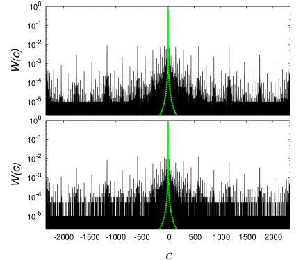
Figure 3: (Color online) The global probability distribution $W(c)$, $c=a$, as defined in Eq. (19), averaged over $N_{R}=10$ realizations of random static imperfections, for $N=493$, $x=2$, $r=56$, $\epsilon=0.04$, disorder realizations are identical for top and bottom panels. The top panel corresponds to the complete computation of Shor’s algorithm as in garcia2007 using in total $27$ qubits, the bottom panel corresponds to the histogram computed using $N_{\rm meas}\sim 12\,000$ measurements (error tolerance $\sim 2\%$ for the associated inverse participation ratio) in the simulation of Shor’s single qubit algorithm with in total $10$ qubits. The grey/green dashed line corresponds to the probability at $\epsilon=0$.

The single qubit Shor algorithm is advantageous for the computation of the inverse participation ratio $\xi$ provided $\xi$ is not too large because this requires less measurement series samples than for the full histogram to achieve a reasonable accuracy. However, a simple replacement of $W(a)$ by the histogram probabilities in (20) is not very optimal for modest sample numbers $N_{R}$ since the average of $\xi^{-1}$ (with $\xi$ obtained from histogram probabilities) scales with the sample number and is not identical with the exact value of $\xi^{-1}$ (with $\xi$ obtained from the exact probabilities $W(a)$). In appendix A we describe a numerical extrapolation scheme that allows to take this into account and to determine a more accurate value of $\xi$ for a finite sample number and also to control its statistical variance. The numerical results of $\xi$ presented in the following have been obtained by this extrapolation scheme and choosing a sample number to achieve a 2% precision.

In Fig. 4 we show the dependence of $\xi$ on the strength of imperfections $\epsilon$. The values of $\xi$ are obtained by the full simulation of Shor’s algorithm as in garcia2007 and by the simulation of the single qubit Shor algorithm using the extrapolation scheme. We see that both methods give very close results even for large values of $\xi$. Thus we may use the more efficient single qubit algorithm to test effects of imperfections for factorization of numbers $N$ much larger than those of garcia2007 .

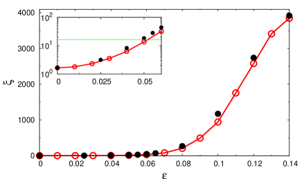
Figure 4: (Color online) Averaged IPR $\xi$ given by (20) as a function of $\epsilon$ for $N=493$, $x=2$. The full circles symbol correspond to the simulation of the full Shor algorithm used in garcia2007 with the complete control register, therefore $n_{\rm tot}=27$. The open circles correspond to the IPR obtained by the single qubit Shor algorithm with the total number of qubits $L=n_{q}+1=10$ and the extrapolation scheme with an error tolerance of 2% that required about $N_{\rm meas}\sim 12000$ measurements. The inset shows the dependence for small $\epsilon$ values, the horizontal dashed line marks the quantum chaos border defined by the condition $\xi(\epsilon_{c})=10\,\xi(0)$. There are $N_{R}=10$ disorder realizations which are identical for full and open circles.

The results of Figs. 3,4 show that with the increase of imperfections strength $\epsilon$ the peak in the distribution $W(a)$ is washed out and the quantum chaos destroys the operability of the algorithm. As in garcia2007 the critical strength of the imperfections $\epsilon_{c}$ at the quantum chaos border can be approximately determined by the condition $\xi(\epsilon_{c})=10\xi(\epsilon=0)$. In Fig. 5 we show the dependence of $\epsilon_{c}$ on the number $N$ factorized by Shor’s algorithm in a log-log scale. The dependence on $N$ can be described as

$$\epsilon_{c}=\frac{B}{(\log_{2}N)^{\beta}}$$ (21)

with numerical constants $B$ and $\beta$. The fit of numerical data done for large $N$ values in the interval $5.5\leq\log_{2}N\leq 18$ gives $B=0.7877\pm 0.073$, $\beta=1.275\pm 0.045$ for the generic imperfection model and $B=0.958\pm 0.154$, $\beta=1.546\pm 0.08$ for the correlated imperfection model. The values for the exponent $\beta$ differ slightly from those obtained in garcia2007 where we had $\beta=1.420\pm 0.054$ for the generic imperfection model and $\beta=1.523\pm 0.068$ for the correlated imperfection model. In view of strong fluctuations related to the arithmetic properties of $x,\,r$ and $N$ we can consider that the agreement with the results obtained in garcia2007 for not very large values of $N<1000$ is rather good. The new data allowed to increase the values of $N\leq 205193$ by a significant factor 200 that gives more accurate values of the exponent $\beta$. The obtained values of $\beta$ are close to the values given by the theoretical estimates garcia2007 with $\beta=1$ for the generic imperfection model and $\beta=1.5$ for the correlated imperfection model. We attribute the deviations of numerical values of $\beta$ from the theoretical values to strong arithmetical fluctuations which require a large scale of $\log_{2}N$-variation. We also note that the statistical fluctuations related to randomness and disorder in realizations of imperfections are relatively small since the standard deviation from disorder average gives an error bar which is approximately of the symbol size in Fig. 5 (the same is true for the data of garcia2007 ).

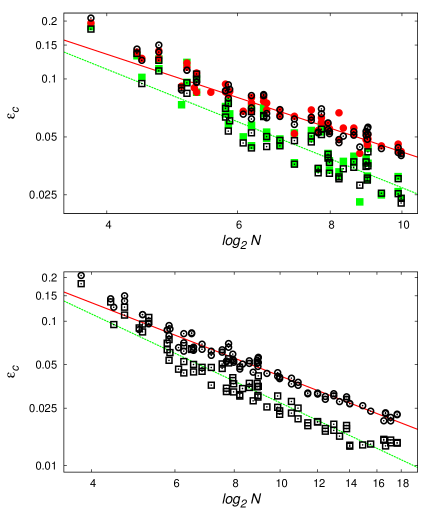
Figure 5: Dependence of the critical imperfections strength $\epsilon_{c}$ on $\log_{2}N$ in log-log scale, $\epsilon_{c}$ is obtained from the criterion $\xi(\epsilon_{c})=10\xi(\epsilon=0)$, where $\xi$ is the inverse participation ratio (20). The top panel shows the results obtained in garcia2007 marked by full symbols (full, red, circles are for the generic imperfection model; full, green, squares are for the correlated imperfection model) and the results of this work marked by open symbols (open circles: the generic imperfection model; open squares: the correlated imperfection model). The bottom panel shows the data of this work up to $N=205193$ (open symbels). The straight lines show the fits $\epsilon_{c}=B/(\log_{2}N)^{\beta}$ of open symbols data for the two models of imperfections in the interval $5.5\leq\log_{2}N\leq 18$ with $B=0.7877\pm 0.073$, $\beta=1.275\pm 0.045$ for the generic imperfection model (solid, red, line), $B=0.958\pm 0.154$, $\beta=1.546\pm 0.08$ for the correlated imperfection model (dashed, green, line).

To give more information we present the results and parameters of our numerical simulations in the Table 1 for large $N$ values $10^{3}\leq N\leq 2\cdot 10^{5}$ which were inaccessible in Ref. garcia2007 .

Table 1: Table for the values of $\epsilon_{c}$ plotted in Fig. 5, for values of $N$ greater than the ones of garcia2007 . In Fig. 5 we see that below $N\approx 1000$ the values of $\epsilon_{c}$ quite well coincide with the ones computed previously in garcia2007 . For simplicity of the table we rounded the numbers to three significant digits. Number of realizations $N_{R}$ is approximate. The number of measurements $N_{\rm meas}$ gives the order of magnitude of the maximum number of measurements for both imperfections models (generic ⁽¹⁾ and correlated ⁽²⁾ imperfection models). Here $L=n_{q}+1$ is the total number of qubits.

$N$	$L$	$\epsilon_{c}^{(1)}$	$\epsilon_{c}^{(2)}$	$x$	$r$	$N_{R}$	$N_{\rm meas}$
1007	11	0.04	0.023	4	234	30	$1\times 10^{6}$
1517	12	0.037	0.023	2	90	15	$5\times 10^{5}$
1517	12	0.040	0.028	3	72	15	$3\times 10^{5}$
1927	12	0.036	0.021	2	460	15	$1\times 10^{5}$
1927	12	0.038	0.025	3	184	15	$4\times 10^{5}$
2773	13	0.032	0.020	2	1334	15	$5\times 10^{5}$
2773	13	0.031	0.019	3	667	15	$6\times 10^{5}$
4087	13	0.032	0.020	2	660	16	$2\times 10^{6}$
4087	13	0.031	0.020	4	330	16	$2.5\times 10^{6}$
5609	14	0.029	0.017	2	1365	15	$1.5\times 10^{6}$
5609	14	0.030	0.018	3	2730	15	$1.5\times 10^{6}$
8051	14	0.031	0.019	2	1968	15	$2.5\times 10^{6}$
8051	14	0.030	0.017	4	984	15	$2\times 10^{6}$
10403	15	0.028	0.016	2	5100	6	$2\times 10^{6}$
14351	15	0.030	0.019	2	28	15	$6\times 10^{5}$
14351	15	0.029	0.018	3	1008	15	$1\times 10^{6}$
16631	16	0.027	0.014	2	1663	4	$2.7\times 10^{6}$
16631	16	0.027	0.014	3	8315	4	$2.1\times 10^{6}$
31313	16	0.026	0.014	2	7740	15	$2.1\times 10^{6}$
47053	17	0.024	0.014	2	7770	3	$1.8\times 10^{6}$
95477	18	0.020	0.015	2	15810	10	$3.7\times 10^{5}$
104927	18	0.023	0.015	2	4740	8	$6.6\times 10^{5}$
141367	19	0.020	0.014	2	23436	3	$3.8\times 10^{5}$
141367	19	0.021	0.015	4	11718	3	$3.8\times 10^{5}$
205193	19	0.022	0.014	2	4256	3	$5\times 10^{5}$
205193	19	0.022	0.014	4	2128	4	$5.1\times 10^{5}$

IV Conclusion

The extensive numerical simulations performed in this work allowed to analyze the accuracy and operability bounds for Shor’s algorithm in presence of realistic static imperfections. The results show that above the quantum chaos border $\epsilon_{c}$ given by Eq. 21 the algorithm becomes not operational while below the border the factorization can be performed. This border drops only polynomially with the logarithm of factorized number $N$. The algebraic power $\beta$ of this decay is close to the theoretical estimates obtained in garcia2007 . The numerical values of $\beta$ are close to the values obtained in garcia2007 where the factorization was studied for significantly smaller values of $N$ compared to the present work. Due to that we think that our results give the real asymptotic value of the algebraic exponent $\beta$ for the quantum chaos border in Shor’s algorithm in presence of static imperfections. Even if the values of $\beta=1$ or $1.5$ are relatively low still the accuracy requirements for quantum gates become rather restrictive if one wants to factorize such large $N$ values as those used in classical computers (see more detailed discussion in garcia2007 ).

This work was supported in part by the EC IST-FET project EuroSQIP. For numerical simulations we used the codes of Quantware Library qwlib .

Appendix A Efficient numerical determination of the IPR for a discrete random variable

Let us consider a discrete random variable $x$ with possible values $x=0,\,1,\,\ldots,\,Q-1$ and probabilities $p(x)\geq 0$ properly normalized $\sum_{x}p(x)=1$. The inverse participation ratio of $x$ is defined as:

$$\frac{1}{\xi}=\sum_{x}p^{2}(x)\ .$$ (22)

Here $\xi$ denotes roughly the number of possible $x$ values with a significant (“maximal”) probability. In the case of quantum states $|\psi\rangle=\sum_{x}\psi(x)\,|x\rangle$ with $p(x)=|\psi(x)|^{2}$ the quantity $\xi$ is also refereed as the (inverse participation ratio) localization length. Obviously, $\xi$ is easily computed provided the exact probabilities $p(x)$ are known. In Ref. garcia2007 , this was indeed the case since we were able to calculate the full quantum state after application of Shor’s algorithm but before measuring the control space variable. However, in this work, where we use the one-control-qubit version of this algorithm as described in section II, this is no longer possible since the exact values of $p(x)$ are not known and we are “only” able to draw an arbitrary number of values $x_{j}$, $j=1,\,\ldots,\,R$ using this probability distribution by simply repeating the one-control-qubit Shor algorithm $R$ times. In the limit $R\to\infty$ this should in principle allow to recover $p(x)$ and $\xi$ with sufficient accuracy but for “moderate” values of $R$ (e. g.: $R\approx 10\xi-100\xi$) this is not very precise and can be improved by a kind of extrapolation scheme in $R$ which we will now explain.

Suppose that $x_{1},\,\ldots,\,x_{R}$ are independent random variables with the same (unknown) probability distribution $p(x)$. For a given set of $x_{1},\,\ldots,\,x_{R}$ (representing “numerically obtained values”) we introduce the histogram probabilities by:

$$p_{R}(x)=\frac{1}{R}\,n_{\{x_{j}\}}=\frac{1}{R}\sum_{j=1}^{R}\,\delta_{xx_{j}}$$ (23)

where $n_{\{x_{j}\}}$ is the number of $x_{j}$ values being equal to $x$. Obviously the average of $\delta_{xx_{j}}$ with respect to $x_{j}$ is: $\langle\delta_{xx_{j}}\rangle=\sum_{x_{j}}p(x_{j})\,\delta_{xx_{j}}=p(x)$ and therefore $\langle p_{R}(x)\rangle=p(x)$. For this simple quantity the average histogram value indeed coincides with the exact value. However, this is not the case for other quantities. Let us for example consider the IPR value obtained by the histogram probabilities:

$$\frac{1}{\xi_{R}}=\sum_{x}p_{R}^{2}(x)$$ (24)

with the following average:

$$\left\langle\frac{1}{\xi_{R}}\right\rangle = \sum_{x}\left\langle p_{R}^{2}(x)\right\rangle=\sum_{x}\frac{1}{R^{2}}\left\langle\sum_{j,l=1}^{R}\delta_{xx_{j}}\,\delta_{xx_{l}}\right\rangle=$$ (25)

$$= \sum_{x}\left(\frac{1}{R}\,p(x)+\frac{R-1}{R}\,p^{2}(x)\right)$$

$$= \rho+(1-\rho)\frac{1}{\xi}\quad{\rm with}\quad\rho=\frac{1}{R}\ .$$

Here the first term arises from the $(j=l)$- and the second term from the $(j\neq l)$-contributions. Wee see that for a finite ratio $R/\xi$ the average histogram-IPR does not coincide with the exact IPR. Eq. (25) allows for the numerical extrapolation:

$$\xi_{\infty}=\xi_{R}\,\frac{1-1/R}{1-\xi_{R}/R}=\xi_{R}\,\frac{1-\rho}{1-\rho\,\xi_{R}}$$ (26)

where $\xi_{R}$ is the numerical histogram-IPR of which we hope that it is close to its average (for large enough $R$) thus justifying (26). This extrapolated IPR will be more reliable than the histogram-IPR for moderate values of $R$ and allow for a more accurate determination of the functional dependence of the IPR on the different parameters. However, $\xi_{\infty}$ is still subject to statistical errors and therefore we also need to compute the variance of the histogram-IPR and related to this we also need the average of the second order histogram-IPR:

$$\frac{1}{\xi_{2,R}}=\sum_{x}\,p_{R}^{3}(x)$$ (27)

as compared to the exact second order IPR:

$$\frac{1}{\xi_{2}}=\sum_{x}\,p^{3}(x)\ .$$ (28)

This quantity is comparable to $1/\xi^{2}$. Actually, using Cauchy-Schwartz inequality (for two vectors $v_{x}=p(x)^{1/2}$ and $w_{x}=p(x)^{3/2}$) we find:

$$\frac{1}{\xi_{2}}=\langle v|v\rangle\langle w|w\rangle\geq|\langle v|w\rangle|^{2}=\frac{1}{\xi^{2}}$$ (29)

with the standard scalar product: $\langle v|w\rangle=\sum_{x}\,v_{x}\,w_{w}$. In Eq. (29) we have equality if $p(x)=$const.$>0$ for certain values of $x$ and $p(x)=0$ for the other values of $x$.

Repeating the calculation (25) for the second order IPR we find:

$$\left\langle\frac{1}{\xi_{2,R}}\right\rangle = \sum_{x}\left\langle p_{R}^{3}(x)\right\rangle=\frac{1}{R^{3}}\sum_{x}\left\langle\sum_{j,l,k=1}^{R}\delta_{xx_{j}}\,\delta_{xx_{l}}\,\delta_{xx_{k}}\right\rangle$$ (30)

$$= \frac{1}{R^{3}}\sum_{x}\Bigl{(}R\,p(x)+3R(R-1)\,p^{2}(x)+$$

$$+R(R-1)(R-2)\,p^{3}(x)\Bigr{)}$$

$$= \rho^{2}+3\,\rho(1-\rho)\frac{1}{\xi}+(1-\rho)(1-2\,\rho)\frac{1}{\xi}_{2}$$

where the three contributions correspond to the cases where the three values $j$, $l$ and $k$ are equal, or only two of them or none of them are equal.

The evaluation of the variance of the histogram-IPR is more complicated but straight forward:

$$\left\langle\frac{1}{\xi_{R}^{2}}\right\rangle=\sum_{x}f_{1}(x)+\sum_{x\neq y}f_{2}(x,y)$$ (31)

with:

$$f_{1}(x) = \left\langle p_{R}^{4}(x)\right\rangle$$

$$= \rho^{3}\,p(x)+7\,\rho^{2}(1-\rho)\,p^{2}(x)+$$

$$+6\,\rho(1-\rho)(1-2\rho)\,p^{3}(x)+$$

$$+(1-\rho)(1-2\rho)(1-3\rho)\,p^{4}(x)\ .$$

We note that the prefactor “7” in the second term of (A) arises from 4 permutations of the type $j=l=k\neq m$ and 3 permutations of the type $j=l\neq k=m$ in the summation index. The prefactor “6” in the third term arises from 6 permutations of the type $j=l\neq k\neq m$.

Furthermore for $x\neq y$ we obtain:

$$f_{2}(x,y) = \left\langle p_{R}^{2}(x)\,p_{R}^{2}(y)\right\rangle$$

$$= \rho^{2}(1-\rho)\,p(x)\,p(y)+$$

$$+\rho(1-\rho)(1-2\rho)\,\left[p^{2}(x)\,p(y)+p(x)\,p^{2}(y)\right]$$

$$+(1-\rho)(1-2\rho)(1-3\rho)\,p^{2}(x)\,p^{2}(y)$$

and therefore:

$$\left\langle\frac{1}{\xi_{R}^{2}}\right\rangle-\left\langle\frac{1}{\xi_{R}}\right\rangle^{2} = 2\,\rho^{2}(1-\rho)\left(\frac{1}{\xi}-\frac{1}{\xi^{2}}\right)+$$

$$+4\,\rho(1-\rho)(1-2\rho)\left(\frac{1}{\xi_{2}}-\frac{1}{\xi^{2}}\right)\ .$$

In the numerical scheme we determine $\xi_{R}^{-1}$ and $\xi_{2,R}^{-1}$ for one realization of $x_{1},\,\ldots,\,x_{R}$ and using (25), (30) we determine approximate values of $\xi^{-1}$ and $\xi_{2}^{-1}$ and by (A) the variance of $\xi_{R}^{-1}$. The number $R$ of $x_{j}$-values is increased until the relative error is below a certain threshold, typically 2%. We note that according to (A) for the special case $\xi_{2}=\xi^{2}$ the variance scales with $\rho^{2}=R^{-2}$ and not with the usual behavior $\rho=R^{-1}$. Even for $\xi_{2}<\xi^{2}$ the numerical prefactor of the $R^{-1}$ term may be quite suppressed as compared to the $R^{-2}$-term and therefore it is better to be careful and not to neglect this term in (A).

References

- (1) P. W. Shor, in Proc. 35th Annu. Symp. Foundations of Computer Science, edited by S. Goldwasser (IEEE Computer Society, Los Alamitos, CA, 1994).
- (2) M. A. Nielsen and I. L. Chuang Quantum Computation and Quantum Information, Cambridge Univ. Press, Cambridge (2000).
- (3) L. M. K. Vanderspyen, M. Steffen, G. Breyta, C. S. Yannoni, M. H. Sherwood, and I. L. Chuang, Nature 414, 883 (2001).
- (4) J.I. Cirac and P. Zoller, Phys. Rev. Lett. 74, 4091 (1995).
- (5) C. Miquel, J. P. Paz, and R. Perazzo, Phys. Rev A 54, 2605 (1996).
- (6) C.Miquel, J.P.Paz and W.H.Zurek, Phys. Rev. Lett. 78, 3971 (1997).
- (7) L.F. Wei, X.Li, X. Hu, and F. Nori, Phys. Rev. A 71, 022317 (2005).
- (8) S.J. Devitt, A.G. Fowler, and L.C.L. Hollenberg, Quant. Info. Comp. 6, 616 (2006).
- (9) R. B. Griffiths and C. S. Niu, Phys. Rev. Lett. 76, 3228 (1996).
- (10) M. Mosca, and A. Ekert, Lecture Notes in Comp. Sci. (Springer) 1509, 174 (1999); quant-ph/9903071.
- (11) C. Zalka, quant-ph/9806084 (1998).
- (12) S. Parker, and M.B. Plenio, Phys. Rev. Lett. 85, 3049 (2000).
- (13) S. Beauregard, Quant. Info. Comp. 3, 175 (2003).
- (14) A.G. Fowler, S.J. Devitt, and L.C.L. Hollenberg, Quant. Info. Comp. 4, 237 (2004).
- (15) B. Georgeot and D. L. Shepelyansky, Phys. Rev. E 62, 3504 (2000); ibid. 62, 6366 (2000).
- (16) K. M. Frahm, R. Fleckinger and D. L. Shepelyansky, Eur. Phys. J. D 29, 139 (2004).
- (17) I. Garcia-Mata, K. M. Frahm, and D. L. Shepelyansky, Phys. Rev. A 75, 052311 (2007); ibid. 76, 039904(E) (2007).
- (18) V. Vedral, A. Barenco and A. Ekert, Phys. Rev. A 54, 147 (1996).
- (19) D. Beckman, A.N. Chari, S. Devabhaktuni, and J. Preskill, Phys. Rev. A 54, 1034 (1996).
- (20) P. Gossett, quant-ph/9808061 (1998).
- (21) T.G. Draper, S.A. Kutin, E.M. Rains, and K.M. Svore, Quant. Info. Comp. 6, 351 (2006).
- (22) R. Van Meter and K.M. Itoh, Phys. Rev. A 71, 052320 (2005).
- (23) C. Zalka, quant-ph/0601097 (2006).
- (24) K. M. Frahm and D. L. Shepelyansky (Eds.), Quantware Library: Quantum Numerical Recipes, http://www.quantware.ups-tlse.fr/QWLIB/ .