The Modulational Instability for a Generalized Korteveg-DeVries equation

Abstract

We study the spectral stability of a family of periodic standing wave solutions to the generalized KdV (g-KdV) in a neighborhood of the origin in the spectral plane using what amounts to a rigorous Whitham modulation theory calculation. In particular we are interested in understanding the role played by the null directions of the linearized operator in the stability of the traveling wave to perturbations of long wavelength.

A study of the normal form of the characteristic polynomial of the monodromy map (the periodic Evan’s function) in a neighborhood of the origin in the spectral plane leads to two different instability indices. The first index counts modulo $2$ the total number of periodic eigenvalues on the real axis. This index is a generalization of the one which governs the stability of the solitary wave. The second index provides a necessary and sufficient condition for the existence of a long-wavelength instability. This index is essentially the quantity calculated by Hǎrǎguş and Kapitula in the small amplitude limit. Both of these quantities can be expressed in terms of the map between the constants of integration for the ordinary differential equation defining the traveling waves and the conserved quantities of the partial differential equation. These two indices together provide a good deal of information about the spectrum of the linearized operator.

We sketch the connection of this calculation to a study of the linearized operator - in particular we perform a perturbation calculation in terms of the Floquet parameter. This suggests a geometric interpretation attached to the vanishing of the modulational instability index previously mentioned.

1 Introduction and Preliminaries

In this paper, we consider standing wave solutions to the generalized KdV (gKdV) equation

$$u_{t}=u_{xxx}+\left(f(u)\right)_{x}-cu_{x}$$ (1)

where $f(\cdot)\in C^{2}(\mathbb{R})$ is a prescribed nonlinearity and $c$ is the wavespeed. Such solutions represent traveling wave solutions to the generalized KdV equation with nonlinearity $f(u)$. Of particular interest is the case of power law nonlinearity $f(u)=u^{p+1}$, which in the cases of $p=1,2$ represents the equations for traveling wave solutions to the KdV and MKdV, respectively. Obviously such traveling wave solutions are reducible to quadrature: they satisfy

$$u_{xx}+f(u)-cu =a$$ (2)

$$\frac{u_{x}^{2}}{2}+F(u)-c\frac{u^{2}}{2} =au+E.$$ (3)

We are interested in the spectrum of the linearized operator (in the moving coordinate frame)

$$\mu v=v_{xxx}+(vf^{\prime}(u))_{x}-cv_{x}$$

in two related settings. First, we study the spectrum in a neighborhood of $\lambda=0$. Physically this amounts to long-wavelength perturbations of the underlying wave profile: in essence slow modulations of the traveling wave. There is a well developed physical theory, commonly known as Whitham modulation theory[40, 41], for dealing with such problems. On a mathematical level the origin in the spectral plane is distinguished by the fact that the ordinary differential equation giving the traveling wave profile is completely integrable. Thus the tangent space to the manifold of traveling wave profiles can be explicitly computed, and the null-space to the linearized operator can be built up from elements of this tangent space. We show that these considerations give a rigorous normal form for the spectrum of the linearized operator in the vicinity of the origin providing that certain genericity conditions are met. Assuming that these genericity conditions are met we are able to show the following: there is a discriminant $\Delta$ which can be calculated explicitly. If this discriminant is positive then the spectrum in a neighborhood of the origin consists of the imaginary axis with multiplicity three. If this discriminant is negative the spectrum of the linearization in the neighborhood of the origin consists of the imaginary axis (with multiplity one) together with two curves which leave the origin along lines in the complex plane, implying instability. Long wavelength theories are invariably geometric in nature, and the one presented here is no exception: both the instability index and the genericity conditions admit a natural geometric interpretation.

Secondly, we are interested in determining sufficient conditions for the existence of unstable spectrum supported away from $\lambda=0$. Here, this is accomplished by calculating an orientation index using Evans function techniques: essentially comparing the behavior of the Evans function near the origin with the asymptotic behavior near infinity. Physically, such an instability amounts to an instability with respect to finite wavelength perturbations. The derived stability index is a generalization of the one which governs stability of solitary waves. In fact, in the case of power-law nonlinearity and wave speed $c>0$, we show that in a long wavelength limit the sign of this index, which is actually what determines stability, agrees with the sign of the solitary wave stability index derived by, for example, Pego and Weinstein[35, 34].

This paper uses ideas from both stability theory and modulation theory, and thus there is an extensive background literature. Most obviously is the stability theory of solitary wave solutions to KdV type equations which was pioneered by Benjamin[4] and further developed by Bona[6], Grillakis[18], Grillakis,Shatah and Strauss[19],Bona, Souganides and Strauss[7], Pego and Weinstein[35, 34], Weinstein[38, 39] and others. In this theory the role of the discriminant is played by the derivative of the momentum with respect to wave-speed. Our discriminant is somewhat more complicated, which is to be expected: the solitary waves homoclinic to the origin are a codimension two subset of the family of periodic solutions, so one expects that the general stability condition will more complicated. There are also a number of calculations of the stability of periodic solutions to perturbations of the same period, or to perturbations of twice the period, due to Angulo Pava[1], Angulo Pava, Bona and Scialom[2] and others. In this setting the linearized operator has a compact resolvent, so the spectrum is purely discrete, and the arguments are similar in spirit to those for the solitary wave stability. In contrast we consider the case of a general $L_{2}$ case where one must understand the continuous spectrum of the operator.

A stability calculation in the spirit of modulation theory was given by Rowlands[36] for the cubic nonlinear Schrödinger equation. Other stability calculations in the same spirit, but differing greatly in details and approach, were given by Gallay and Hǎrǎguş[15, 16], Hǎrǎguş and Kapitula[21], Bridges and Rowlands[11], and Bridges and Mielke[10]. The work of Gardner[17] is also related, though it should be noted that the long-wavelength limit in Gardner is very different from the one we consider here: in the former it is the traveling wave itself which has a long period. In our calculation the period is fixed and we are considering perturbations of long period. The current paper also owes a debt to the substantial literature on Whitham theory for integrable systems developed by Lax and Levermore[28, 26, 27], Flashka, Forest and McLaughlin[14], and many others. We note, however, that the calculation outlined in this paper is not an integrable calculation. The papers that are perhaps closest to that presented here are those by Oh and Zumbrun[31, 32, 33] and Serre[37] on the stability of periodic solutions to viscous conservation laws, where similar results relating the behavior of the linearized spectral problem in a neighborhood of the origin to a formal theory of slow modulations are proved.

Our results are most explicit in the case of power law nonlinearity. It should be noted that due to the scaling invariance in this case we can always assume that $c\in\{-1,+1\}$. Indeed, it is easy to check that if $u(x,t;c)$ solves (1) with the nonlinearity $f(u)=u^{p+1}$, then

$$u(x,t;c)=|c|^{1/p}u\left(|c|^{1/2}x,|c|^{3/2}t,\operatorname{sgn}(c)\right)$$ (4)

solves (1) with wave speed $\operatorname{sgn}(c)$.

The paper is organized as follows: in the second section we lay out some basic general properties of the spectrum of the linearized operator. In the third section we explicitly compute the monodromy map and associated periodic Evan’s function at the origin. A perturbation analysis in the neighborhood of the origin gives a normal form for the Evan’s function. In the fourth section we develop similar results from the point of view of the linearized operator: we compute the generalized null-space of the linearized operator in terms of the tangent space to the ordinary differential equation defining the traveling wave. The structure of this null-space (under some genericity conditions) reflects that of the monodromy map at the origin, and a similar perturbation analysis gives a normal form for the spectrum. While the two approaches are in principle the same most of the calculations are more easily carried out in the context of the monodromy map/Evans function. We mainly present the calculations at the level of the linearized operator since it helps to clarify some aspects of the monodromy calculation. Finally we end with some concluding remarks.

It should be noted we restrict neither the size of the periodic solution nor the period. Moreover, all of our analysis applies to both localized and bounded perturbations of the underlying wave. Also in this paper “stability” will always means spectral stability.

1.1 Preliminaries

Note that the partial differential equation has (in general) three conserved quantities

$$M =\int_{0}^{T}u(x,t)dx$$

$$P =\int_{0}^{T}u^{2}(x,t)dx$$

$$H =\int_{0}^{T}\frac{1}{2}u_{x}^{2}+F(u)dx$$

which correspond to the mass, momentum and Hamiltonian of the solution respectively. These quantities considered as functions of the traveling waves parameters will form an important part of the analysis.

The periodic standing wave solutions of (1) are of the form $u(x,t)=u(x)$ where $u$ is a periodic function in the x-variable. Substituting this into (1) and integrating twice we see that $u$ satisfies

$$\frac{1}{2}u_{x}^{2}+F\left(u\right)-\frac{c}{2}u^{2}-au=E$$ (5)

where $a,E\in\mathbb{R}$ are constants of integration and $F^{\prime}=f$. Note that the solitary wave case corresponds to $a=0,E=0,$ so the solitary waves are a codimension two subset of the periodic waves. In order to assure the existence of a periodic orbits, we must require that the effective potential

$$V(u;a,c)=F(u)-\frac{c}{2}u^{2}-au$$

has a local minimum. Note that this places a condition on the allowable parameter regime $\mathcal{D}$ for our problem. We will always assume that we are in the interior of this open region, and that the roots $u_{+},u_{-}$ of the equation $V(u;a,c)=E$ with $V(u;a,c)<E$ for $u\in(u_{-},u_{+})$ are simple, guaranteeing that they are $C^{1}$ functions of $a,E,c$.

As is standard, the the period of the corresponding periodic orbit is given by

$$T=T(a,E,c):=2\int_{u_{-}}^{u_{+}}\frac{du}{\sqrt{2\left(E-V(u;a,c)\right)}}.$$ (6)

The above interval can be regularized at the square root branch points $u_{-},\;u_{+}$ by the following procedure: Write $E-V(u;a,c)=(r-u_{-})(u_{+}-r)Q(u)$ and consider the change of variables $u=\frac{u_{+}+u_{-}}{2}+\frac{u_{+}-u_{-}}{2}\sin(\theta)$. Notice that $Q(u)\neq 0$ on $[u_{-},u_{+}]$. It follows that $du=\sqrt{(u-u_{-})(u_{+}-u)}d\theta$ and hence (6) can be written in a regularized form as

$$T(a,E,c)=2\int_{-\frac{\pi}{2}}^{\frac{\pi}{2}}\frac{d\theta}{\sqrt{Q\left(\frac{u_{+}+u_{-}}{2}+\frac{u_{+}-u_{-}}{2}\sin(\theta)\right)}}.$$

Similarly the mass, momentum, and Hamiltonian of the traveling wave are given by the first and second moments of this density, i.e.

$$M(a,E,c)=\langle u\rangle =\int_{0}^{T}u(x)dx=2\int_{u_{-}}^{u_{+}}\frac{u\;du}{\sqrt{2\left(E-V(u;a,c)\right)}}$$

$$P(a,E,c)=\langle u^{2}\rangle =\int_{0}^{T}u^{2}(x)dx=2\int_{u_{-}}^{u_{+}}\frac{u^{2}\;du}{\sqrt{2\left(E-V(u;a,c)\right)}}$$

$$H(a,E,c)=\left\langle\frac{u_{x}^{2}}{2}-F(u)\right\rangle =2\int_{u_{-}}^{u_{+}}\frac{E-V(u;a,c)-F(u)}{\sqrt{2\left(E-V(u;a,c)\right)}}\;du.$$

Notice that these integrals are regularized by the same substitution. In particular one can differentiate the above expressions with respect to the parameters $(a,E,c)$ and the derivatives of these quantities will play an important role in the subsequent theory. Note that there is a third constant of integration $x_{0}$ corresponding to translation invariance, but this can be modded out and does not play an important role in the theory.

These quantities satisfy a number of identities, as is derived in the appendix. In particular if we define the classical action

$$K=\oint p\;dq=\int_{0}^{T}u_{x}^{2}\;dx=2\int_{u_{-}}^{u_{+}}\sqrt{2(E-V(u;a,c))}\;du$$

(which is not itself conserved) then this quantity satisfies the following relations

$$K_{E} =T$$

$$K_{a} =M$$

$$K_{c} =\frac{P}{2}.$$

Using the fact that $T,M,P$ and $H$ are $C^{1}$ functions of parameters $(a,E;c)$, the above implies the following relationship between the gradients of these quantities

$$E\nabla T+a\nabla M+\frac{c}{2}\nabla P+\nabla H=0$$

where $\nabla=(\partial_{a},\partial_{E},\partial_{c})$: see the appendix for details of this calculation. The subsequent theory is developed most naturally in terms of the quantities $T$, $M$, and $P$. However, it is possible to restate our results in terms of $M$, $P$ and $H$ using the above identity. This is desirable since these have a natural interpretation as conserved quantities of the partial differential equation.

As noted before this long-wavelength calculation is geometric, and a number of Jacobian determinants arise. We adopt the following notation for $2\times 2$ Jacobians

$$\{f,g\}_{x,y}=\left|\begin{array}[]{cc}f_{x}&g_{x}\\ f_{y}&g_{y}\end{array}\right|$$

with $\{f,g,h\}_{x,y,z}$ representing the analogous $3\times 3$ Jacobian.

We now begin our study of linear stability of the periodic waves $u(x)=u(x;a,E,c)$ under small perturbation. To this end, we consider a small perturbation of the periodic wave $u(x;a,E)$ of the form

$$\psi(x,t;a,E,c)=u(x;a,E,c)+\varepsilon v(x,t)+O(\varepsilon^{2}),$$

where $0<|\varepsilon|\ll 1$ is a small parameter. Substituting this into (1) and collecting the $O(\varepsilon)$ terms yields the linearized equation $\partial_{x}\mathcal{L}[u]v=-v_{t}$, where $\mathcal{L}[u]:=-\partial_{x}^{2}-f^{\prime}(u)+c$ is a linear differential operator with periodic coefficients. Since the linearized equation is autonomous in time, we may seek separated solutions of the form $v(x,t)=e^{-\mu t}v(x)$, which yields the eigenvalue problem

$$\partial_{x}\mathcal{L}[u]v=\mu v.$$ (7)

Note that we consider the linearized operator $\partial_{x}\mathcal{L}[u]$ as a closed linear operator acting on a Banach space $X$ with domain $\mathcal{D}(\partial_{x}\mathcal{L}[u])$. In literature, several choices for $X$ have been studied, each of which corresponding to different classes of admissible perturbations $v$. In our case, we consider $X=L^{2}(\mathbb{R};\mathbb{R})$ and $\mathcal{D}(\partial_{x}\mathcal{L}[u])=H^{3}(\mathbb{R})$, corresponding to spatially localized perturbations. In this case standard Floquet theory yields the following definitions.

Definition 1.

The monodromy matrix $\,\mbox{\bf M}(\mu)$ is defined to be the period map

$$\,\mbox{\bf M}(\mu)=\Phi(T,\mu)$$

where $\Phi(x,\mu)$ satisfies

$$\Phi_{x}=\,\mbox{\bf H}(x;\mu)\Phi~{}~{}~{}~{}~{}~{}~{}~{}~{}~{}\Phi(0,\mu)={\bf I}$$ (8)

with ${\bf I}$ the $3\times 3$ identity matrix and

$$\,\mbox{\bf H}(x;\mu)=\left(\begin{array}[]{ccc}0&1&0\\ 0&0&1\\ -\mu-u_{x}f^{\prime\prime}(u)&-f^{\prime}(u)+c&0\\ \end{array}\right).$$

Given the monodromy the spectrum is characterized as follows:

Definition 2.

We say $\mu\in\operatorname{spec}(\partial_{x}\mathcal{L}[u])$ if there exists a non-trivial bounded function $\psi$ such that $\partial_{x}\mathcal{L}[u]\psi=\mu\psi$ or, equivalently if there exists a $\lambda\in\mathbb{C}$ such that $|\lambda|=1$ and

$$\det[\,\mbox{\bf M}(\mu)-\lambda{\bf I}]=0.$$

Following Gardner[17] we define the periodic Evans function to be

$$D(\mu,\lambda)=\det\left(\,\mbox{\bf M}(\mu)-\lambda{\bf I}\right).$$ (9)

Moreover, we say the periodic solution $u(x;a,E,c)$ is spectrally stable if $\operatorname{spec}(\partial_{x}\mathcal{L}[u])$ does not intersect the open right half plane.

Remark 1.

Notice that due to the Hamiltonian nature of the problem, $\operatorname{spec}(\partial_{x}\mathcal{L}[u])$ is symmetric with respect to reflections across the real and imaginary axes. Thus, spectral stability occurs if and only if $\operatorname{spec}(\partial_{x}\mathcal{L}[u])\subset\mathbb{R}i$. Since we are primarily concerned with roots of $D(\mu,\lambda)$ with $\lambda$ on the unit circle we will frequently work with the function $D(\mu,e^{i\kappa})$, which is actually the function considered by Gardner.

In this paper, we will study different asymptotics of this function. In the next section, we will study the asymptotics of (9) as $\mu\to\infty$. This will provide information about the global structure of the spectrum of the linearized operator $\partial_{x}\mathcal{L}[u]$, as well as providing us with a finite wavelength instability index which counts modulo 2 the number of intersections of the spectrum with the positive real axis. We then study the asymptotics of (9) in the limit $(\mu,\kappa)\to(0,0)$, which yields a quantity which we refer to as a modulational stability index, which is expressed in terms of the derivatives of the monodromy operator at the origin.

2 Global Structure of $\operatorname{spec}(\partial_{x}\mathcal{L}[u])$

In this section, we review some basic global features of the spectrum of the linearized operator $\partial_{x}\mathcal{L}[u]$ which are useful in a local analysis near $\mu=0$. We also state some important properties of the Evans function $D(\mu,\lambda)$ which are vital to the foregoing analysis.

Proposition 1.

The spectrum $\operatorname{spec}\left(\partial_{x}{\cal L}[u]\right)$ has the following properties:

• There are no isolated points of the spectrum. In particular, the spectrum consists of piecewise smooth arcs.

• $D(\mu,\lambda)=\det(\,\mbox{\bf M}(\mu)-\lambda{\bf I})=-\lambda^{3}+a(\mu)\lambda^{2}-a(-\mu)\lambda+1$ with $a(\mu)=\,\mbox{\rm tr}(\,\mbox{\bf M}(\mu)).$

• The function $a(\mu)$ satisfies $a(0)=3,a^{\prime}(0)=0.$

• The entire imaginary axis is contained in the spectrum, i.e. $i\mathbb{R}\subset\operatorname{spec}(\partial_{x}\mathcal{L}).$ Further for $|\mu|$ sufficiently large along the imaginary axis the multiplicity is one.

• $\mathbb{R}\cap\operatorname{spec}(\partial_{x}\mathcal{L})$ consists of a finite number of points. In particular there are no bands on the real axis.

Proof.

The first claim, that the spectrum is never discrete, follows from a basic lemma in the theory of several complex variables: namely that, if for fixed $\lambda^{*}$ the function $D(\mu,\lambda^{*})$ has a zero of order $k$ at $\mu^{*}$ and is holomorphic in a polydisc about $(\mu^{*},\lambda^{*})$ then there is some smaller polydisc about $(\mu^{*},\lambda^{*})$ so that for every $\lambda$ in a disc about $\lambda^{*}$ the function $D(\mu,\lambda)$ (with $\lambda$ fixed) has $k$ roots in the disc $|\mu-\mu^{*}|<\delta$. For details see the text of Gunning[20]. It is clear from the implicit function theorem that $\mu$ is a smooth function of $\lambda$ as long as $\frac{\partial D}{\partial\mu}=\,\mbox{\rm tr}(\operatorname{cof}^{t}(\,\mbox{\bf M}(\mu)-\lambda{\bf I})\,\mbox{\bf M}_{\mu}^{\prime})\neq 0,$ where $\operatorname{cof}$ represents the standard cofactor matrix.

The second claim is an easy symmetry calculation. The stability problem is invariant under the the map $x\mapsto-x,\mu\mapsto-\mu,$ which implies that

$$\,\mbox{\bf M}(\mu)\sim{\,\mbox{\bf M}}^{-1}(-\mu).$$

Thus one has

$$\det[\,\mbox{\bf M}(-\mu)-\lambda{\bf I}] = \det[{\,\mbox{\bf M}}^{-1}(\mu)-\lambda{\bf I}]$$

$$= -\lambda^{3}\det[{\,\mbox{\bf M}}^{-1}(\mu)]\det[\,\mbox{\bf M}(\mu)-\lambda^{-1}]$$

$$= -\lambda^{3}\left(-\lambda^{-3}+a(\mu)\lambda^{-2}+b(\mu)\lambda^{-1}+1\right)$$

$$= -\lambda^{3}-b(\mu)\lambda^{2}-a(\mu)\lambda+1$$

from which it follows $b(\mu)=-a(-\mu)$.

The proof of the third claim will be deferred until lemma 2.

The fourth claim is another symmetry argument. Since $a(\mu)$ is real on the real axis it follows from Schwarz reflection that for $\mu\in\mathbb{R}i$, we have $a(-\mu)=a(\overline{\mu})=\overline{a(\mu)}$ and the characteristic polynomial takes the form

$$D(\mu,\lambda)=-\lambda^{3}+a\lambda^{2}-\overline{a}\lambda+1$$

where $a=a(\mu)$, and thus

$$D(\mu,\lambda)=-\lambda^{3}\overline{D\left(\mu;\overline{\lambda}^{-1}\right)}.$$

Hence for imaginary $\mu$ the eigenvalues of the monodromy are symmetric with respect to the unit circle with the same multiplicities. Since the monodromy has three eigenvalues, it follows that at least one must lie on the unit circle.

To see that the multiplicity is eventually one we note that by standard asymptotics the monodromy $\,\mbox{\bf M}(\mu)$ satisfies

$$\,\mbox{\bf M}(\mu)\approx e^{{\bf A}(\mu)T},~{}~{}~{}~{}~{}~{}|\mu|\gg 1$$

where ${\bf A}(\mu)$ is defined by

$${\bf A}(\mu)=\left(\begin{array}[]{ccc}0&1&0\\ 0&0&1\\ -\mu&0&0\\ \end{array}\right).$$

The three eigenvalues of $e^{{\bf A}(\mu)T}$ are given by

$$\lambda_{1}=e^{-\mu^{1/3}T},\;\;\lambda_{2}=e^{-\mu^{1/3}\omega T},\;\;\rm{and}\;\;\lambda_{3}=e^{-\mu^{1/3}\overline{\omega}T}$$ (10)

where $\omega=e^{2\pi i/3}$ is the principle third root of unity. If $\mu\in\mathbb{R}^{+}i$ it follows that $\lambda_{1}=\exp\left(-|\mu|^{1/3}e^{i\pi/6}T\right)$ and since $\cos(\pi/6)>0$ we have $|\lambda_{1}|\to 0$ as $\mathbb{R}^{+}i\ni\mu\to\infty$. Similarly, $\lambda_{2}=\exp\left(-|\mu|^{1/3}e^{5\pi/6}T\right)$ and $\lambda_{3}=\exp\left(|\mu|^{1/3}i\right)$ so that $|\lambda_{2}|\to\infty$ as $\mathbb{R}^{+}i\ni\mu\to\infty$ and $|\lambda_{3}|=1$. Thus, for $\mu\in\mathbb{R}^{+}i$ large, we have that $\mu$ is an eigenvalue of multiplicity one. Similarly, we can show $|\lambda_{1}|\to\infty$, $|\lambda_{3}|\to 0$ as $\mathbb{R}^{+}i\ni\mu\to-\infty$ and $|\lambda_{2}|=1$ for $\mu\in\mathbb{R}^{-}i$, $|\mu|\gg 1$. Therefore, it follows that $\mu\in\operatorname{spec}(\partial_{x}\mathcal{L}[u])$ with multiplicity one for $\mu\in\mathbb{R}i$, $|\mu|\gg 1$.

The final claim follows from a similar asymptotic calculation together with an analyticity argument. Notice that for $\mu$ real the eigenvalues of the monodromy are either all real or one real and one complex conjugate pair. If the eigenvalues lie on the unit circle then in the first case $1$ or $-1$ must be an eigenvalue. In the second one must have a complex conjugate pair of eigenvalues, and thus (since the determinant is one) $1$ must be an eigenvalue. Thus if a point on the real axis is in the spectrum then either $\det(\,\mbox{\bf M}(\mu)-{\bf I})$ or $\det(\,\mbox{\bf M}(\mu)+{\bf I})$ must vanish. Since $\det(\,\mbox{\bf M}(\mu)\pm{\bf I})$ are entire functions it follows that either they are identically zero or the zero set has not finite accumulation points. The large $\mu$ asymptotics implies that they cannot be identically zero, therefore the zero set must be discrete. Further the large $\mu$ asymptotics implies that for sufficiently large $\mu$ along the real axis $\mu\notin\operatorname{spec}\left(\partial_{x}\mathcal{L}[u]\right)$, so the spectrum is confined to a compact subset of the real line, and there are only a finite number of real eigenvalues. ∎

Remark 2.

Note that, in the calculation of Hǎrǎguş and Kapitula[21] the real eigenvalues play a slightly different role than other eigenvalues off of the imaginary axis. The fact that there are only a finite number of these indicates that there are only a finite number of values of the Floquet parameter for which there are real eigenvalues: $\kappa_{r}(\gamma)=0$ for all but a finite number of values of the Floquet parameter $\gamma$ in their notation.

2.1 Analysis of $\operatorname{spec}(\partial_{x}\mathcal{L}[u])\bigcap\mathbb{R}$

We now move on to study the structure of $\operatorname{spec}(\partial_{x}\mathcal{L}[u])\cap\mathbb{R}$ more carefully. Suppose that $\mu\in\mathbb{R}$. Clearly $1$ being an eigenvalue of $\,\mbox{\bf M}(\mu)$ is a sufficient condition for $\mu\in\operatorname{spec}(\partial_{x}\mathcal{L}[u])$ and thus vanishing of $D(\mu,1)=a(\mu)-a(-\mu)$ is a sufficient condition $\mu\in\operatorname{spec}(\partial_{x}\mathcal{L}[u])\cap\mathbb{R}$. Notice that by the translation invariance of (7) we have $D(0,1)=0$ by Noether’s theorem. The question is whether $D(\mu,1)$ has any other real roots. If it does, then the eigenvalue problem (7) is spectrally unstable, due to the presence of a real non-zero element of $\operatorname{spec}(\partial_{x}\mathcal{L}[u])$. In order to detect this instability, we calculate the orientation index

$$D(\infty,1)D_{\mu\mu\mu}(0,1).$$

As we will show, the negativity of this index is sufficient to imply a non-trivial intersection of $\operatorname{spec}(\partial_{x}\mathcal{L}[u])$ with the real line.

Lemma 1.

The function $D(\;\cdot\;,1):\mathbb{R}\to\mathbb{R}$ is an odd function which satisfies the asymptotic relation

$$\lim_{\mathbb{R}\ni\mu\to\pm\infty}D(\mu,1)=\mp\infty.$$

Proof.

Clearly, $D(\;\cdot\;,1)$ is an odd function of its argument, and hence it is sufficient to consider the limit as $\mu\to\infty$. To begin, define a new variable $\rho=\mu^{1/3}T$. Then from the asymptotic relations (10) we have

$$a(\rho) = e^{-\rho}+e^{-(-1+\sqrt{3}i)\rho/2}+e^{-(-1-\sqrt{3}i)\rho/2}$$

$$\widetilde{a}(\rho) = e^{\rho}+e^{-(1+\sqrt{3}i)\rho/2}+e^{-(1-\sqrt{3}i)\rho/2}$$

where $\widetilde{a}(\rho)$ is the trace when you take $\mu\to-\mu$. It follows that $D(\mu,1)=a(\rho)-\widetilde{a}(\rho)$ behaves like $-e^{\rho}$ for large positive $\rho$, i.e. $\mu\gg 0$. This completes the proof. ∎

From these results, we have the following theorem relating the sign of $\,\mbox{\rm tr}(\,\mbox{\bf M}_{\mu\mu\mu}(0))$ to the stability of the underlying periodic wave.

Theorem 1.

If $a^{\prime\prime\prime}(0)=\,\mbox{\rm tr}(\,\mbox{\bf M}_{\mu\mu\mu}(0))>0$, then the number of roots of $D(\mu,1)$ (i.e. the number of periodic eigenvalues) on the positive real axis is odd. In particular $\operatorname{spec}(\partial_{x}\mathcal{L}[u])\cap\mathbb{R}^{*}\neq\emptyset$ and the eigenvalue problem (7) is spectrally unstable.

Proof.

We show in Lemma 2 that $D(0,1)=D_{\mu}(0,1)=D_{\mu\mu}(0,1)=0$ and $D_{\mu\mu\mu}(0,1)=2a^{\prime\prime\prime}(0)$. Thus, if $a^{\prime\prime\prime}(0)>0$, then $D(\mu;1)$ is positive for small positive values of $\mu$. Since $D(\mu,1)$ is negative for sufficiently large $\mu$ we know that $D(\pm\mu^{*},0)=0$ for some $\mu^{*}\in\mathbb{R}\setminus\{0\}$, which completes the proof. In the next section we establish the following formula for $D_{\mu\mu\mu}(0,1)$, the first non-vanishing derivative

$$D_{\mu\mu\mu}(0,1)=-3\left|\begin{array}[]{ccc}T_{a}&M_{a}&P_{a}\\ T_{E}&M_{E}&P_{E}\\ T_{c}&M_{c}&P_{c}\end{array}\right|=6\left|\begin{array}[]{ccc}K_{aa}&K_{aE}&K_{ac}\\ K_{aE}&K_{EE}&K_{cE}\\ K_{ac}&K_{cE}&K_{cc}\end{array}\right|=\frac{3}{E}\left|\begin{array}[]{ccc}M_{a}&P_{a}&H_{a}\\ M_{E}&P_{E}&H_{E}\\ M_{c}&P_{c}&H_{c}\end{array}\right|$$

where again $K$ is the classical action of the traveling wave ODE. Hence this “orientation index” can be expressed in terms of the Jacobian of the map between the constants of integration of the traveling wave ordinary differential equation $(a,E;c)$ and the conserved quantities of the g-KdV $(M,P,H).$ This orientation index is analogous to the quantity which is calculated in the stability theory of the solitary waves. ∎

It is important to notice the instability detected by Theorem 1 is an instability with respect to finite (bounded) wavelength perturbations. In the next section we will derive a modulational stability index which detects instability with respect to arbitrarily long wavelength perturbations. See the comments at the end of the section 3. The solitary wave solutions go unstable in the manner detected by Theorem 1, through the creation of a pair of eigenvalues on the real axis. In general the periodic waves seem to first go unstable through the creation of a curve of spectrum which does not intersect the real axis, and later there is a secondary bifurcation resulting in a real eigenvalue. This phenomenon appears to have first been observed by Kapitula and Hǎrǎguş, who established that small amplitude periodic waves first go unstable at $p=2$, as compared with $p=4$ for the solitary waves. While we don’t have a general proof of this we do show that, in the case of power law nonlinearity, there is a real periodic eigenvalue as well as a band of unstable spectrum connected to the origin. It is also worth noting that the analogous calculation for $D(\mu,-1)$ shows that the number of anti-periodic eigenvalues on the real axis is always even. While this is not useful for proving the existence of instabilities it does eliminate some possible modes of instability.

3 Local Analysis of the Period Map

In this section, we turn our attention to studying the monodromy map $\,\mbox{\bf M}(\mu)$ near the origin. To this end, we determine the asymptotic behavior of $D(\mu,e^{i\kappa})$ as $\mu\to 0$. We begin by proving that $D(0,e^{i\kappa})$ has a zero of multiplicity three at $\kappa=0$. It follows by directly computing the Jordan normal form of $\,\mbox{\bf M}(0)$ that $\lambda=1$ is an eigenvalue of algebraic multiplicity three and geometric multiplicity (generically) two. This fact reflects the following structure in the manifold of solutions to the ordinary differential equation defining the traveling waves: the traveling waves form a three parameter manifold, with traveling waves of constant period forming a two parameter submanifold. The two eigenvectors of the period map correspond to elements of the tangent plane to the submanifold of constant period solutions, while the third vector in the Jordan chain is associated to the normal to the constant period submanifold.

Using perturbation theory appropriate to a Jordan block, as well as the Hamiltonian symmetry inherent in (7), we prove the three roots of $D(\mu,e^{i\kappa})$ bifurcate from $\mu=0$ analytically in $\kappa$ in a neighborhood of $\kappa=0$, and derive a necessary and sufficient condition for modulational instability of the underlying periodic wave $u(x;a,E,c)$ in terms of derivatives of the monodromy operator. Note that this conclusion is somewhat unexpected: normally the eigenvalues of a non-trivial Jordan block do not bifurcate analytically but instead admit a Puiseaux series in fractional powers. However because of the symmetries of the problem the admissible perturbations are severely restricted, resulting in a non-generic bifurcation.

3.1 Calculation of the Period Map

The first major calculation we present is an explicit calculation of the monodromy matrix at the origin in terms of the derivatives of the underlying periodic solution $u$ with respect to the parameters. We do this by first computing a matrix valued solution to the ordinary differential equation satisfying the wrong initial condition: ${\bf U}(0,0)$ is non-singular but not the identity. One can then multiply on the right by ${\bf U}^{-1}(0,0)$ to find the monodromy matrix. We find that (as expected) the monodromy operator $\,\mbox{\bf M}(\mu)$ has a non-trivial Jordan form when $\mu=0$. Our goal is then to utilize perturbation theory of Jordan blocks to calculate the normal form of the characteristic polynomial in a neighborhood of $\mu=0,\;\lambda=1$, where $\lambda$ is the eigenvalue parameter of the monodromy operator.

To begin we write the above third order eigenvalue problem as a first order system as in (8). In particular, notice that $\,\mbox{\rm tr}(\,\mbox{\bf H}(x;\mu))=0$ for all $x,\mu$, and thus $\det(\Phi(x;\mu))=1$ for all $\mu\in\mathbb{C}$, implying $\det(\,\mbox{\bf M}(\mu))=1$. In order to calculate a matrix solution $\Phi(x;\mu)$, we must first find three linearly independent solutions of the above system. In general, this is a daunting task, but since the above system with $\mu=0$ arises as the Frechet derivative (linearization) of an integrable ordinary differential equation this can be done by considering infinitesimal variations of the constants of integration in the defining ordinary differential equation, and thus generating the tangent space. As noted earlier the solutions $u(x-x_{0};a,E,c)$ constitute a 4-dimensional solution manifold of (1) parameterized by $x_{0},a,E,c$. The solutions of the linearized operator space are given by the generators $\frac{d}{dx}$, $\frac{d}{da}$, and $\frac{d}{dE}$ acting on the solution $u(x;a,E,c)$. The action of the generator $\frac{d}{dc}$ is somewhat different and is connected with the generalized null-space. This will become important in the next section.

Proposition 2.

Let $u(x;a,E,c)$ be the solution to the traveling wave equation (5) satisfying $u(0;a,E,c)=u_{-},u_{x}(0;a,E,c)=0.$ A basis of solutions to the third order system

$$Y_{x}=\,\mbox{\bf H}(x;0)Y$$

is given by

$$Y_{1}^{t}=(u_{x},u_{xx},u_{xxx})$$

$$Y_{2}^{t}=(u_{a},u_{ax},u_{axx})$$

$$Y_{3}^{t}=(u_{E},u_{Ex},u_{Exx}).$$

A particular solution to the inhomogeneous problem

$$Y_{x}=\,\mbox{\bf H}(x;0)Y+W$$

where $W^{t}=(0,0,u_{x})$ is given by

$$Y_{3}^{t}=(u_{c},u_{cx},u_{cxx}).$$

Proof.

A straightforward calculation. Notice that it follows that $\partial_{x}\mathcal{L}[u]\left(-u_{c}\right)=u_{x}$. ∎

The fact that $u_{a},u_{E}$ are not periodic - they exhibit secular growth due to the variation of the period with respect to the parameters - gives an indication that the eigenspaces of the monodromy at $\mu=0$ are not semi-simple, and hence we expect the existence of a non-trivial Jordan block of the monodromy map $\,\mbox{\bf M}(0)$.

By the above proposition, three linearly independent solutions of (8) corresponding to $\mu=0$ are given by

$$Y_{1}(x)=\left(\begin{array}[]{c}u^{\prime}(x;a,E,c)\\ u^{\prime\prime}(x;a,E,c)\\ u^{\prime\prime\prime}(x;a,E,c)\\ \end{array}\right)\;\;\;Y_{2}(x)=\left(\begin{array}[]{c}u_{a}(x;a,E,c)\\ u_{a}^{\prime}(x;a,E,c)\\ u_{a}^{\prime\prime}(x;a,E,c)\\ \end{array}\right)\;\;\;Y_{3}(x)=\left(\begin{array}[]{c}u_{E}(x;a,E,c)\\ u_{E}^{\prime}(x;a,E,c)\\ u_{E}^{\prime\prime}(x;a,E,c)\\ \end{array}\right).$$ (11)

By hypothesis, for any $a,E,c\in\mathbb{R}$ the solution $u$ satisfies

$$u(0;a,E,c) = u_{-}\;=\;u(T;a,E,c)$$ (12)

$$\partial_{x}u(0;a,E,c) = 0\;=\;\partial_{x}u(T;a,E,c)$$ (13)

$$\partial_{xx}u(0;a,E,c) = a-f(u_{-})+cu_{-}\;=\;\partial_{xx}u(T;a,E,c).$$ (14)

Moreover, from equation (1) it follows that

$$u_{xxx}(0;a,E,c)=cu_{x}(0;a,E,c)-\frac{d}{dx}\left(f(u(x;a,E,c))\right)\big{|}_{x=0}=0.$$

Defining $\,\mbox{\bf U}(x,0)=[Y_{1}(x),Y_{2}(x),Y_{3}(x)]$ to be the corresponding solution matrix, then direct calculations yield

$$\,\mbox{\bf U}(0,0)=\left(\begin{array}[]{ccc}0&\partial_{a}u_{-}&\partial_{E}u_{-}\\ a-f(u_{-})+cu_{-}&0&0\\ 0&1+(c-f^{\prime}(u_{-}))\partial_{a}u_{-}&(c-f^{\prime}(u_{-}))\partial_{E}u_{-}\end{array}\right).$$ (15)

Note that differentiating the relation $E-V(u_{-})=0$ gives the relation $-V^{\prime}(u_{-})\partial_{E}u_{-}=\det(\,\mbox{\bf U}(0,0))=-1$, so these solutions are linearly independent at $x=0$, and hence for all $x$. Thus we can compute ${\bf U}(T,0)$ and right-multiply by ${\bf U}^{-1}(0,0)$ to give the monodromy ${\bf M}(0)$

The matrix $\,\mbox{\bf U}(T,0)$ can be calculated by differentiating (12)-(14) with respect to the parameters $a$ and $E$ by use of the chain rule. For example, differentiating the relation (12) with respect to the parameter $E$ gives

$$\partial_{E}u(T;a,c,E)+\frac{\partial u}{\partial x}\left(T;a,E,c\right)T_{E}(a,c,E)=\partial_{E}u_{-}.$$

Since the derivative vanishes at the period points this implies $\partial_{E}u(T)=\partial_{E}u_{-}$. Continuing in this manner gives the following expression for the change in tis matrix solution across the period:

$$\,\mbox{\bf U}(T,0)=\,\mbox{\bf U}(0,0)+\left(\begin{array}[]{ccc}0&0&0\\ 0&V^{\prime}(u_{-};a,c)T_{a}&V^{\prime}(u_{-};a,c)T_{E}\\ 0&0&0\end{array}\right).$$ (16)

In particular, we find that $\,\mbox{\bf U}(T,0)-\,\mbox{\bf U}(0,0)$ is a rank one matrix, which naturally leads to the following proposition.

Proposition 3.

There exists a basis in $\mathbb{R}^{3}$ such that the monodromy matrix $M(\mu)$ evaluated at $\mu=0$ takes the following Jordan normal form:

$$\,\mbox{\bf M}(0)\sim\left(\begin{array}[]{ccc}1&0&0\\ 0&1&\sigma\\ 0&0&1\end{array}\right)$$ (17)

where $\sigma\neq 0$ as long as $T_{a}$ and $T_{E}$ do not simultaneously vanish. In particular, the monodromy operator at $\mu=0$ has a single eigenvalue of $\lambda=1$ with algebraic multiplicity three and geometric multiplicity two as long as the period is not at a critical point with respect to the parameters $a,E$ for fixed wavespeed $c$.

Proof.

Recall $\det(\,\mbox{\bf U}(0,0))=-V^{\prime}(u_{-})\partial_{E}u_{-}=-1$, so $\,\mbox{\bf U}(0,0)$ is invertible. Multiplying the above expression on the right by the matrix $\,\mbox{\bf U}^{-1}(0,0)$ yields the monodromy matrix at the origin

$$\,\mbox{\bf M}(\mu=0):=I+\vec{w}\otimes\vec{v}\;\,\mbox{\bf U}^{-1}(0)$$

where $\vec{w}=(0,1,0)^{T}$ and $\vec{v}=\left(0,V^{\prime}(u_{-})T_{a},V^{\prime}(u_{-})T_{E}\right)^{T}$. Next, notice that

$$\,\mbox{\bf U}(0,0)\left(\begin{array}[]{ccc}0&-T_{a}&-T_{E}\\ 0&0&0\\ 0&0&0\end{array}\right)=\vec{w}\otimes\vec{v}$$

and hence defining $\,\mbox{\bf N}:=\,\mbox{\bf U}^{-1}(0)\,\mbox{\bf M}(0)\,\mbox{\bf U}(0)$ gives the equation

$$\,\mbox{\bf N}=\left(\begin{array}[]{ccc}1&-T_{a}&-T_{E}\\ 0&1&0\\ 0&0&1\end{array}\right).$$

It follows that

$$Ker(\,\mbox{\bf N}-{\bf I})=span\left\{(1,0,0)^{T},\;(0,T_{E},-T_{a})^{T}\right\}$$

Now, take $\vec{v_{3}}:=(0,-T_{a},-T_{E})$ and notice that $v_{3}\notin Ker(\,\mbox{\bf N}-{\bf I})$. The Jordan structure then follows by noticing then that $(\,\mbox{\bf N}-{\bf I})\vec{v_{3}}=(T_{a}^{2}+T_{E}^{2})(1,0,0)^{T}\in\ker({\bf N}-{\bf I})$.

For traveling waves below the separatrix a result of Schaaf (see appendix) shows that the period is a strictly increasing function of the energy, $T_{E}>0$ and thus the genericity condition is always met. In other situations we will assume that this condition is met unless otherwise stated. ∎

3.2 Asymptotic Analysis of $D(\mu,\kappa)$ near $(\mu,\kappa)=(0,0)$

We now analyze the characteristic polynomial of $\,\mbox{\bf M}(\mu)$ in a neighborhood of $\mu=0$ by considering $\,\mbox{\bf M}(\mu)$ as a small perturbation of the matrix $\,\mbox{\bf M}(0)$ constructed above. It is well understood how the eigenvalues of a Jordan block bifurcate under perturbation: see Kato[25] or Moro, Burke and Overton[30]. It is worth noting, however, that in this case the bifurcation is highly non-generic due to the constraints imposed by the symmetry of the problem.

Recall from Proposition 1 that the spectrum near $\mu=0$ is continuous. By the analyticity of $\,\mbox{\bf M}(\mu)$ in a neighborhood of $\mu=0$, we can expand $\,\mbox{\bf M}(\mu)$ for small $\mu$ as

$$\,\mbox{\bf M}(\mu)=\,\mbox{\bf M}(0)+\mu\,\mbox{\bf M}_{\mu}(0)+\frac{\mu^{2}}{2}\,\mbox{\bf M}_{\mu\mu}(0)+\mathcal{O}\left(|\mu|^{3}\right)$$

where $\,\mbox{\bf M}_{\mu}(0)=[M^{(1)}_{i,j}]$ and $\,\mbox{\bf M}_{\mu\mu}(0)=[M^{(2)}_{i,j}]$. If one makes a similarity transform $\widetilde{\,}\mbox{\bf M}(\mu)={\bf V}^{-1}\,\mbox{\bf M}(\mu){\bf V}$ so that $\widetilde{\,}\mbox{\bf M}(0)$ is in the Jordan normal form (17) then a direct calculation using the above second order expansion of $\widetilde{\,}\mbox{\bf M}(\mu)$ implies that in a neighborhood of $\mu=0$, the characteristic polynomial can be expressed as

$$D(\mu,e^{i\kappa}) = \det\left((\widetilde{\,}\mbox{\bf M}(\mu)-I)-(e^{i\kappa}-1){\bf I}\right)$$ (18)

$$= -\eta^{3}+\eta^{2}\left(\mu\,\mbox{\rm tr}\left(\widetilde{\,}\mbox{\bf M}_{\mu}(0)\right)+\frac{\mu^{2}}{2}\,\mbox{\rm tr}(\widetilde{\,}\mbox{\bf M}_{\mu\mu}(0))\right)$$

$$- \eta\left(\mu{\widetilde{M}}^{(1)}_{3,2}\sigma+\mu^{2}\left(\frac{1}{2}\left(\,\mbox{\rm tr}(\widetilde{\,}\mbox{\bf M}_{\mu})\right)^{2}-\frac{1}{2}\,\mbox{\rm tr}(\widetilde{\,}\mbox{\bf M}_{\mu}^{2})-\frac{\sigma}{2}{\widetilde{M}}^{(2)}_{3,2}\right)\right)$$

$$- \sigma(\widetilde{M}^{(1)}_{1,1}\widetilde{M}^{(1)}_{3,2}-\widetilde{M}^{(1)}_{3,1}\widetilde{M}^{(1)}_{1,2})\mu^{2}$$

$$+ \mu^{3}\left(\det\left(\widetilde{\,}\mbox{\bf M}_{\mu}(0)\right)+\sigma S\right)+\mathcal{O}\left(4\right),$$

where $\eta=e^{i\kappa}-1$, $S$ represents mixed terms from $\widetilde{\,}\mbox{\bf M}_{\mu}(0)$ and $\widetilde{\,}\mbox{\bf M}_{\mu\mu}(0)$, $\sigma$ is as in Proposition 3, and the notation $\mathcal{O}\left(4\right)$ represents terms whose degree is four or higher. Notice there are no other $\mu^{3}$ terms since $\,\mbox{\bf M}(0)-I$ has rank one. Our next goal is to determine the dominant balance of the equation $D(\mu,e^{i\kappa})=0$ in a neighborhood of $(\mu,\kappa)=(0,0)$.

A useful construction for implicit function calculations of this type is that of the Newton diagram, which is a subset of the non-negative integer lattice. A vertex $(i,j)$ is included if the coefficient of $\eta^{3-i}\mu^{j}$ in (18) is non-zero, otherwise the vertex is not included. The lower convex hull of the Newton diagram is made up of a collection of line segments. For each line segment of the lower convex hull let $m$ be the horizontal length of the segment and $s$ the slope of the segment. Corresponding to each such line segment there are $m$ distinct solution branches of the form

$$\eta_{k}(\mu)=\sum_{i}\alpha^{(k)}_{i}\mu^{si},$$

where $\alpha^{(k)}_{1}\neq 0$ and $k$ ranges from $1$ to $m$. For details see the book of Baumgartel[3] or Hilton[22]. This is equivalent to the method of “dominant balance” presented in textbooks on asymptotic methods but is somewhat more systematic. For instance, in our case if the coefficient of the $\eta^{1}\mu^{1}$ term (-$\sigma\tilde{M}^{(1)}_{3,2}$) is non-vanishing then there are two solution branches in which $\eta$ has an expansion in powers of $\mu^{\frac{1}{2}}$ and one with an expansion in integer powers. These correspond to the breaking up of the $2\times 2$ and $1\times 1$ Jordan blocks respectively. However as mentioned above the symmetry $\,\mbox{\bf M}(\mu)\sim\,\mbox{\bf M}^{-1}(-\mu)$ causes a number of terms in (18) to vanish, which leads to an expansion in integer powers of $\mu$. This is the content of the next lemma.

Lemma 2.

The equation $D(\mu,e^{i\kappa})=0$ has the following normal form in a neighborhood of $(\mu,\kappa)=(0,0)$:

$$-(i\kappa)^{3}+\frac{i\kappa\mu^{2}}{2}\,\mbox{\rm tr}\left(\,\mbox{\bf M}_{\mu\mu}(0)\right)+\frac{\mu^{3}}{3}\,\mbox{\rm tr}\left(\,\mbox{\bf M}_{\mu\mu\mu}(0)\right)+O(4)=0$$

whose Newton diagram is depicted in Figure 2.

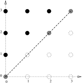
Figure 1: The Newton diagram corresponding to the asymptotic expansion of $D(\mu,e^{i\kappa})=0$ in a neighborhood of $(\mu,\kappa)=(0,0)$ is shown to $O(|\mu|^{3})$. Terms associated to open circles are shown to vanish due to the natural symmetries inherent in (1). The grey circles are non-vanishing terms which are a part of the lower convex hull. The black circles lie above the lower convex hull and thus do not contribute to the leading order asymptotics.

Proof.

Define functions a, b, c on a neighborhood of $\mu=0$ by

$$\det[(\,\mbox{\bf M}(\mu)-I)-(e^{i\kappa}-1)I]=-\eta^{3}+(a(\mu)-3)\eta^{2}+b(\mu)\eta+c(\mu).$$ (19)

where $\eta=e^{i\kappa}-1$. Notice in particular that $\eta=i\kappa+\mathcal{O}\left(\kappa^{2}\right)$ in a neighborhood of $\kappa=0$. By (18), it follows

$$a(\mu) = \,\mbox{\rm tr}(\,\mbox{\bf M}(\mu))=3+\mu\,\mbox{\rm tr}(\,\mbox{\bf M}_{\mu}(0))+\frac{\mu^{2}}{2}\,\mbox{\rm tr}(\,\mbox{\bf M}_{\mu\mu}(0))+\frac{\mu^{3}}{6}\,\mbox{\rm tr}(\,\mbox{\bf M}_{\mu\mu\mu}(0))+\mathcal{O}(|\mu|^{4})$$

$$b(\mu) = \frac{1}{2}\left(\,\mbox{\rm tr}((\,\mbox{\bf M}(\mu)-I)^{2})-\,\mbox{\rm tr}(\,\mbox{\bf M}(\mu)-I)^{2}\right)=-\mu M^{(1)}_{3,2}\sigma-\mu^{2}\left(\frac{1}{2}\,\mbox{\rm tr}(\,\mbox{\bf M}_{\mu})^{2}-\frac{1}{2}\,\mbox{\rm tr}(\,\mbox{\bf M}_{\mu}^{2})-\frac{\sigma}{2}\tilde{M}_{3,2}\right)+\mathcal{O}(|\mu|^{3})$$

$$c(\mu) = \det(\,\mbox{\bf M}(\mu)-I)=-\sigma(M^{(1)}_{1,1}M^{(1)}_{3,2}-M^{(1)}_{3,1}M^{(1)}_{1,2})\mu^{2}+\left(\det(\,\mbox{\bf M}_{\mu}(0))+\sigma S\right)+\mathcal{O}(|\mu|^{4})$$

Using the symmetry $\,\mbox{\bf M}(-\mu)\sim\,\mbox{\bf M}(\mu)^{-1}$, we have

$$c(-\mu) = \det[\,\mbox{\bf M}(-\mu)-I]$$

$$= \det[\,\mbox{\bf M}(\mu)]^{-1}\det[I-\,\mbox{\bf M}(\mu)]$$

$$= -\det[\,\mbox{\bf M}(\mu)-I]$$

$$= -c(\mu)$$

since $\det[\,\mbox{\bf M}(\mu)]=1$ for all $\mu\in\mathbb{C}$. Hence $c$ is an odd function of $\mu$. Also, since $\,\mbox{\bf M}(0)-{\bf I}$ has rank one, (18) along with the above analysis implies that $c(\mu)=\mathcal{O}(|\mu|^{3})$, from which it follows $c^{\prime\prime}(0)=-2\sigma(M^{(1)}_{1,1}M^{(1)}_{3,2}-M^{(1)}_{3,1}M^{(1)}_{1,2})=0$.

Similarly, using (19) we have

$$\det[\,\mbox{\bf M}(\mu)-\lambda{\bf I}] = -\lambda^{3}\det\left[\,\mbox{\bf M}(-\mu)-\frac{1}{\lambda}\right]$$

$$= -\lambda^{3}\left(\left(\frac{1}{\lambda}-1\right)^{3}+a(-\mu)\left(\frac{1}{\lambda}-1\right)^{2}+b(-\mu)\left(\frac{1}{\lambda}-1\right)+c(-\mu)\right)$$

$$= -(\lambda-1)^{3}-a(-\mu)\lambda(\lambda-1)^{2}+b(-\mu)\lambda^{2}(\lambda-1)-c(-\mu)\lambda^{3}.$$

Comparing the $\lambda^{2}$ and $\lambda^{3}$ terms above with those in (19) we get the relations

$$\left\{\begin{array}[]{ll}b(\mu)=2a(\mu)-a(-\mu)-3,&\hbox{and}\\ a(\mu)-b(\mu)+c(\mu)=3.&\end{array}\right.$$

Since $c(\mu)=\mathcal{O}(|\mu|^{3})$, these relations imply $\,\mbox{\rm tr}\left(\,\mbox{\bf M}_{\mu}(0)\right)=a^{\prime}(0)=0$ and $-\sigma\tilde{M}^{(1)}_{3,2}=b^{\prime}(0)=0$. By recalling $\sigma\neq 0$ from 3, this implies $\tilde{M}^{(1)}_{3,2}=0$. Moreover, we know that $a^{\prime\prime}(0)=b^{\prime\prime}(0)$ and hence $b^{\prime\prime}(0)=\,\mbox{\rm tr}(\,\mbox{\bf M}_{\mu\mu}(0))$. Also, we have $b^{\prime\prime\prime}(0)=3a^{\prime\prime\prime}(0)$ and $c^{\prime\prime\prime}(0)=b^{\prime\prime\prime}(0)-a^{\prime\prime\prime}(0)=2a^{\prime\prime\prime}(0)$ and hence $c^{\prime\prime\prime}(0)=2\,\mbox{\rm tr}(\,\mbox{\bf M}_{\mu\mu\mu}(0))$. The corollary follows by analyzing equation (18) as well as the corresponding Newton diagram (see Figure 1). ∎

From this it follows that, in the neighborhood of the origin, the leading order piece of the periodic Evans function is a homogeneous cubic polynomial in $\kappa,\mu$. The implicit function theorem fails, but in a trivial way that is easily corrected, leading to the following theorem:

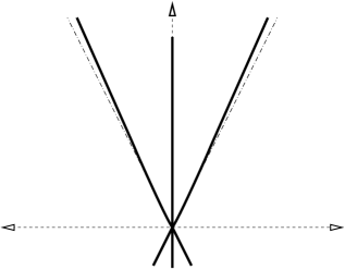
Figure 2: When $\Delta(f;u)<0$, the local normal form of $\operatorname{spec}(\partial_{x}\mathcal{L}[u])$ consists of a segment of the imaginary axis union with two straight lines making equal angles with the imaginary axis. Notice that these lines intersect at the origin, corresponding to the fact that $1$ is an eigenvalue of $\,\mbox{\bf M}(0)$ with algebraic multiplicity three.

Theorem 2.

With the above notation, define

$$\Delta(f;u)=\frac{1}{2}\left(\,\mbox{\rm tr}(\,\mbox{\bf M}_{\mu\mu}(0))\right)^{3}-3\left(\,\mbox{\rm tr}(\,\mbox{\bf M}_{\mu\mu\mu}(0))\right)^{2},$$ (20)

where $f$ denotes the dependence on the non-linearity used in (1), and suppose $\,\mbox{\rm tr}(\,\mbox{\bf M}_{\mu\mu\mu}(0))\neq 0.$ If $\Delta>0$, then the imaginary axis in the neighborhood in the origin is in the spectrum with multiplicity three. If $\Delta<0$ then the imaginary axis in a neighborhood of the origin is in the spectrum with multiplicity one, together with two curves which are tangent to lines through the origin with angle $\arg(iy_{2,3})$ - see Figure 2. In particular in the latter case the periodic wave is modulationally unstable.

Proof.

Since the leading order piece of the Evan’s function is homogeneous it suggests working with a projective coordinate $y=\frac{i\mu}{\kappa}.$ Making such a change of variables leads to the equation

$$1-\frac{y^{2}}{2}\,\mbox{\rm tr}\left(\,\mbox{\bf M}_{\mu\mu}(0)\right)+\frac{y^{3}}{3}\,\mbox{\rm tr}\left(\,\mbox{\bf M}_{\mu\mu\mu}(0)\right)+\kappa E(\kappa,y)=0$$

where $E(\kappa,y)$ is continuous in a neighborhood of the origin. The implicit function theorem applies in a neighborhood of $(y=y_{1,2,3},\kappa=0)$ as long as the roots $y_{1,2,3}$ of the above cubic in $y$ are distinct, which is true as long as the discriminant $\Delta$ is not zero. In terms of the original variable $\mu$ we have the three solution branches

$$\mu_{1,2,3}=iy_{1,2,3}\kappa+O(\kappa^{2})$$

This cubic has three real roots when $\Delta>0$, giving three branches of spectrum emerging from the origin tangent to the imaginary axis. It is clear from symmetry that these must in fact lie on the imaginary axis, giving a interval of spectrum of multiplicity three along the imaginary axis. In the case that the discriminant is negative there is one real root and two complex conjugate roots, giving one branch of spectrum along the imaginary axis and two branches emerging in the complex plane. ∎

Remark 3.

First we note that $\,\mbox{\rm tr}(\,\mbox{\bf M}_{\mu\mu}(0))<0$ is a sufficient condition for modulational instability of the periodic wave.

Secondly we note that the Newton diagram is independent of $\,\mbox{\rm tr}(\,\mbox{\bf M}_{\mu\mu}(0))$ but the dominant balance changes if $\,\mbox{\rm tr}(\,\mbox{\bf M}_{\mu\mu\mu}(0))$ should happen to vanish. Later we will give a formula for $\,\mbox{\rm tr}(\,\mbox{\bf M}_{\mu\mu\mu}(0))$ in terms of the Jacobian of a map, and we will see that vanishing of this quantity signals a change in the Jordan structure of the underlying linearized operator.

Finally we note that this agrees with the result of Bottman and Deconinck[8], in which they considered cnoidal wave solutions to the KdV. Using the algebro-geometric techniques of Belokolos, Bobenko, Enol’skii, Its and Matveev[5] they explicitly computed the spectrum of the linearized operator and found that such solutions are always linearly stable. Their results prove that an interval of the imaginary axis containing the origin is in the spectrum of the linearized operator, with multiplicity three. Our results imply this is a generic phenomenon: either one has an interval of spectrum of multiplicity three about the origin, or one has three curves intersecting at the origin. In the KdV case the discriminant $\Delta$ is expressible in terms of elliptic functions in this case and must be positive, although we have not tried to show this.

It is instructive to compare this theorem with that of Theorem 1. By Theorem 2, the sign of $\,\mbox{\rm tr}(\,\mbox{\bf M}_{\mu\mu\mu}(0))$ has no effect on the spectral stability of the underlying periodic wave in a sufficiently small neighborhood of the origin. However, Theorem 1 guarantees the existence of unstable real spectrum if $\operatorname{sgn}\left(\,\mbox{\rm tr}(\,\mbox{\bf M}_{\mu\mu\mu}(0))\right)>0$. To reconcile these results, notice Proposition (1) implies there is no unstable real spectrum sufficiently close to the origin. Thus, the instability brought on by $\,\mbox{\rm tr}(\,\mbox{\bf M}_{\mu\mu\mu}(0))>0$ is not local to $\mu=0$, and hence should not be detected by the quantity $\Delta(a,E,c)$.

Our next goal is to try to evaluate the modulational stability index $\Delta(a,E,c)$ as well as the finite wavelength orientation index $\,\mbox{\rm tr}(\,\mbox{\bf M}_{\mu\mu\mu}(0))$ in terms of the conserved quantities of (1). This can be done very explicitly. Notice that while we have chosen to express the coefficients as $\,\mbox{\rm tr}(\,\mbox{\bf M}_{\mu\mu}(0))$ and $\,\mbox{\rm tr}(\,\mbox{\bf M}_{\mu\mu\mu}(0))$, which suggests that they arise at second order and third order in a perturbation calculation for small $\mu$, these quantities can be expressed in terms of quantities which arise at first and second order in $\mu$ due to the invariance of the problem under the map $\mu\rightarrow-\mu$. Further while all of the first order terms contribute only a few terms which are second order actually contribute - these are the terms which are associated to the minors of the off-diagonal piece of the unperturbed Jordan form. These second order terms are explicitly computable via a single quadrature.

Theorem 3.

We have the following identities:

$$\,\mbox{\rm tr}(\,\mbox{\bf M}_{\mu\mu})|_{\mu=0} =\{T,P\}_{E,c}+2\{M,P\}_{a,E}$$

$$\,\mbox{\rm tr}(\,\mbox{\bf M}_{\mu\mu\mu})|_{\mu=0} =-\frac{3}{2}\{T,M,P\}_{a,E,c}$$

where $T,M,P$ are the period, mass, and momentum of the underlying traveling wave and $a,E,c$ parameterize the family of traveling waves. Thus the modulational stability index has the following representation

$$\Delta=\frac{1}{2}\left(\{T,P\}_{E,c}+2\{M,P\}_{a,E}\right)^{3}-3\left(\frac{3}{2}\{T,M,P\}_{a,E,c}\right)^{2}.$$

Proof.

Let $w_{i}(x;\mu)$, $i=1,2,3$, be three linearly independent solutions of (1), and let $\,\mbox{\bf W}(x,\mu)$ be the solution matrix with columns $w_{i}$. Expanding the above solutions in powers of $\mu$ as

$$w_{i}(x,\mu)=w_{i}^{0}(x)+\mu w_{i}^{1}(x)+\mu^{2}w_{i}^{2}(x)+\mathcal{O}(|\mu|^{3})$$

and substituting them into (7), the leading order equation becomes

$$\frac{d}{dx}w_{i}^{0}(x)=\,\mbox{\bf H}(x;0)w_{i}^{0}(x).$$

Using Proposition 2, we choose $w_{i}(x)=Y_{i}(x)$ where the vectors $Y_{i}(x)$ are defined in equation (11). The higher order terms in the above expansion yield

$$\frac{d}{dx}w_{i}^{j}(x)=\,\mbox{\bf H}(x;0)w_{i}^{j}(x)+V_{i}^{j-1}(x),\;\;j\geq 1,$$

where $V_{i}^{j-1}=\left(0,0,-(w_{i}^{j-1})_{1}\right)^{t}$ and $(v)_{1}$ denotes the first component of the vector $v$. Notice that for each of the higher order terms $j\geq 1$, we require $w_{j}^{i}(0)=0$. This implies that $\,\mbox{\bf W}(0,\mu)=\,\mbox{\bf U}(0,0)$ in a neighborhood of $\mu=0$, where $\,\mbox{\bf U}(0,0)$ is defined in (15). In the case $j=1$, the $i=1$ equation is equivalent to the equation $L_{0}w_{1}^{1}=u_{x}$. It follows again from Proposition 2 that we can choose

$$w_{1}^{1}(x)=\left(\begin{array}[]{c}-u_{c}\\ -u_{cx}\\ -u_{cxx}\\ \end{array}\right)+u_{-}\left(\begin{array}[]{c}u_{a}\\ u_{a}^{\prime}\\ u_{a}^{\prime\prime}\\ \end{array}\right)-\frac{u_{-}^{2}}{2}\left(\begin{array}[]{c}u_{E}\\ u_{E}^{\prime}\\ u_{E}^{\prime\prime}\\ \end{array}\right).$$

Notice the above coefficients of $Y_{2}(x)$ and $Y_{3}(x)$ are determined by differentiating $E-V(u_{-};a,c)=0$ with respect to the parameters $a$, $E$, and $c$. Moreover, using variation of parameters as well as the identities $\{u_{x},u\}_{x,E}=-1$ and $\{u,u_{x}\}_{x,a}=u$, we choose

$$w_{i}^{j}(x) = \,\mbox{\bf W}(x,0)\int_{0}^{x}\,\mbox{\bf W}(z,0)^{-1}V_{i}^{j-1}(z)dz$$ (24)

$$= \left(\begin{array}[]{ccc}u_{x}\int_{0}^{x}(w_{i}^{j-1})_{1}\{u,u_{x}\}_{a,E}\;dz-u_{a}\int_{0}^{x}(w_{i}^{j-1})_{1}dz+u_{E}\int_{0}^{x}(w_{i}^{j-1})_{1}u\;dz\\ u_{xx}\int_{0}^{x}(w_{i}^{j-1})_{1}\{u,u_{x}\}_{a,E}\;dz-u_{ax}\int_{0}^{x}(w_{i}^{j-1})_{1}dz+u_{Ex}\int_{0}^{x}(w_{i}^{j-1})_{1}u\;dz\\ u_{xxx}\int_{0}^{x}(w_{i}^{j-1})_{1}\{u,u_{x}\}_{a,E}\;dz-u_{axx}\int_{0}^{x}(w_{i}^{j-1})_{1}dz+u_{Exx}\int_{0}^{x}(w_{i}^{j-1})_{1}u\;dz\\ \end{array}\right)$$

for $w_{i}^{1}$, $i=2,3$, and $w_{i}^{j}$ for $i>1$. Finally, by (16), we have the following expression valid as $\mu\to 0$:

$$\delta\,\mbox{\bf W}(\mu)=\left(\begin{array}[]{ccc}\mathcal{O}(|\mu|^{2})&\mathcal{O}(|\mu|)&\mathcal{O}(|\mu|)\\ \mu V^{\prime}(u_{-})\left(-T_{c}+u_{-}T_{a}-\frac{u_{-}^{2}}{2}T_{E}\right)+\mathcal{O}(|\mu|^{2})&V^{\prime}(u_{-})T_{a}+\mathcal{O}(|\mu|)&V^{\prime}(u_{-})T_{E}+\mathcal{O}(|\mu|)\\ \mathcal{O}(|\mu|^{2})&\mathcal{O}(|\mu|)&\mathcal{O}(|\mu|)\\ \end{array}\right),$$

where $\delta\,\mbox{\bf W}(\mu):=\,\mbox{\bf W}(x,\mu)\big{|}_{x=0}^{T}$, and the $\mathcal{O}(\mu)$ and $\mathcal{O}(\mu^{2})$ terms above are computed using (24). Note that all of the $\mathcal{O}(\mu,\mu^{2})$ terms in the above are necessary for the calculation, however we do not write them out. Recalling that our choice of basis implies $\det(\,\mbox{\bf W}(0,\mu))=-1$, we have

$$D(\mu,1) = -\textrm{det}\left(\delta\,\mbox{\bf W}(\mu)\right)$$

$$= -\frac{1}{2}\{T,M,P\}_{a,E,c}\;\mu^{3}+\mathcal{O}(|\mu|^{4}),$$

from which the expression for $\,\mbox{\rm tr}(\,\mbox{\bf M}_{\mu\mu\mu}(0))$ follows by Theorem 1. Moreover, it follows from Lemma 2 and the fact $\,\mbox{\bf M}(\mu)=\delta\,\mbox{\bf W}(\mu)\,\mbox{\bf W}(0,0)^{-1}+{\bf I}$ and a rather tedious calculation that

$$\,\mbox{\rm tr}(\,\mbox{\bf M}_{\mu\mu}(0)) = -2\mu^{-2}\,\mbox{\rm tr}(\textrm{cof}(\,\mbox{\bf M}(\mu)-I))\big{|}_{\mu=0}$$

$$= -2\left(-\frac{1}{2}\{T,P\}_{E,c}-\{M,P\}_{E,a}\right)$$

as claimed. ∎

Corollary 1.

$\{T,M,P\}_{a,E,c}<0$ is a sufficient condition for a non-trivial intersection of $\operatorname{spec}(\partial_{x}\mathcal{L}[u])$ with the real axis.

Proof.

This is now clear from Theorems 1 and 3. ∎

At this point we can make a connection to the stability theory for the solitary waves.

Corollary 2.

In the case of power-law nonlinearity and wavespeed $c>0$, there are always unstable periodic traveling waves in a neighborhood of the solitary wave $(a=E=0)$ if $p>4$. Moreover, such long wavelength periodic waves exhibit a modulational instability if and only if $p>4$.

Proof.

First, note that the scaling invariance in equation (4) implies the periodic solution $u(x;a,E,c)$ satisfies

$$u(x;a,E,c)=c^{1/p}u\left(c^{1/2}x;\frac{a}{c^{1+1/p}},\frac{E}{c^{1+2/p}},1\right),$$

which allows us to compute $T_{c}$, $M_{c}$, $P_{c}$ explicitly as follows:

$$T_{c} =-\frac{1}{2c}T-\frac{a(p+1)}{pc}T_{a}-\frac{E(p+2)}{pc}T_{E}$$

$$M_{c} =\left(\frac{1}{pc}-\frac{1}{2c}\right)M+\left(T_{c}+\frac{T}{2c}\right)u_{-}-\frac{a(p+1)}{pc}\left(M_{a}-T_{a}u_{-}\right)-\frac{E(2+p)}{pc}\left(M_{E}-T_{E}u_{-}\right)$$

$$P_{c} =\left(\frac{2}{pc}-\frac{1}{2c}\right)P+\left(T_{c}+\frac{T}{2c}\right)u_{-}^{2}-\frac{a(p+1)}{pc}\left(P_{a}-T_{a}u_{-}^{2}\right)-\frac{E(2+p)}{pc}\left(P_{E}-T_{E}u_{-}^{2}\right),$$

where $T_{c}$ follows from equation (6). Since we know that $P_{E}=2T_{c}$ and $P_{a}=2M_{c}$ the above serves to simplify the last row and column. When $a$ and $E$ are small there are two turning points $r_{1},r_{2}$ in the neighborhood of the origin and a third turning point $r_{3}$ which is bounded away from the origin. In the solitary wave limit $a,E\rightarrow 0$ we have $r_{1}-r_{2}=O(\sqrt{a^{2}-2E})$. In this limit we have the following asymptotics for small $(a,E)$

$$M(a,E,1) =O(1)$$

$$P(a,E,1) =O(1)$$

$$T(a,E,1) =O\left(\ln(a^{2}-2E)\right)$$

$$T_{a}(a,E,1) =O\left(\frac{a}{a^{2}-2E}\right)=M_{E}$$

$$T_{E}(a,E,1) =O\left(\frac{1}{a^{2}-2E}\right).$$

Thus the asymptotically largest minor of $\{T,M,P\}_{a,E,c}$ is $-T_{E}M_{a}P_{c}$, from which it follows

$$\{T,M,P\}_{a,E,c}\sim-T_{E}M_{a}\left(\frac{2}{pc}-\frac{1}{2c}\right)P$$

as $a,E\to 0$. It is known that for traveling waves below the separatrix (see appendix) that under some minor convexity assumptions $T_{E}>0$. It can also be shown that (see appendix) $M_{a}(a,0)<0$ for $E=0$ and $a$ sufficiently small. Thus the orientation index $\{T,M,P\}_{a,E,c}$ is negative for $p>4$ and $a,E$ sufficiently small (in other words sufficiently close to the solitary wave) and positive for $p<4$ and $a,E$ sufficiently small. This also follows, of course, from Gardner’s long-wavelength theory[17] but it provides a good check for the present theory.

To prove the second claim, notice the above asymptotics implies

$$\,\mbox{\rm tr}(\,\mbox{\bf M}_{\mu\mu}(0)) \sim T_{E}\left(\frac{2}{pc}-\frac{1}{2c}\right)P$$

in the limit as $a,E\to 0$. Hence, it follows that $\operatorname{sgn}\Delta(a,E,c)=\operatorname{sgn}(4-p)$ for $a,$ $E$ sufficiently small, and periodic waves of sufficiently long period are also modulationally unstable for $p>4$.

∎

Remark 4.

It is worth noting that the instability mechanism detected by the discriminant $\Delta$ is not present in the solitary wave case: in the solitary wave limit the bands of spectrum connected to the origin collapse to the origin. This instability does not appear to follow from Gardner’s calculation: Gardner shows that the point eigenvalue of the solitary wave opens into a small loop of spectrum, predicting the real eigenvalues detected by $\{T,M,P\}_{a,E,c},$ but the modulational instability detected by $\Delta$ is not detected. Thus suggests the heuristic that periodic solutions should go unstable before the solitary waves. The small amplitude stability calculation of Hǎrǎguş and Kapitula for the generalized KdV equation amounts to a calculation of this discriminant in that limiting case, and their proof that the small amplitude waves go unstable at $p=2$ is the first result we are aware of along these lines.

We believe that a small amplitude analysis of $\Delta(a,E,c)$ should be possible. It follows by a simple calculation that $\Delta=0$ at the stationary solution. By expanding near by solutions in terms of amplitude instead of the energy $E$, we believe the first non-zero term of the discriminant should be proportional to a polynomial which switches signs at $p=2$, thus recovering the small amplitude result of Hǎrǎguş and Kapitula [21]. We have not as yet carried out such an analysis.

Using the identities derived in Appendix $1$, we now have a sufficient criterion for the existence of a non-trivial intersection of $\operatorname{spec}(\partial_{x}\mathcal{L}[u])$ with the real axis in terms of the conserved quantities $M$, $P$ and $H$ of the gKdV flow, as well as a necessary and sufficient condition for understanding the normal form of the spectrum in a neighborhood of the origin. It is a rather striking fact that both of these indices can be expressed entirely in terms of the conserved quantities of the flow. The monodromy itself depends on $u_{-}(a,E,c)$, the classical turning point of the traveling wave, as well as various functions and derivatives of this quantity, but the indices themselves only depend on the conserved quantities. This is, of course, the Whitham philosophy, but we are only aware of a few cases (other than the integrable calculations, which are very special) in which make this rigorous.

In the next section we outline the connections of this calculation to a calculation based more directly on the linearized operator. While not strictly necessary this calculation is useful since it clarifies the way in which various bifurcations can occur. In this section we calculate the null-space and generalized null-space of the linearized operator and sketch a perturbation calculation analogous to the one given for the Evan’s function.

4 Local Analysis of $\operatorname{spec}(\partial_{x}\mathcal{L}[u])$ via the Floquet-Boch Decomposition

4.1 Floquet-Bloch Decomposition

In this section we sketch an approach to this problem working directly with the linearized operator rather than with the Evan’s function. While these two approaches are presumably equivalent the former seems less straightforward than the latter. In particular it is not clear how one might derive the orientation index in this way, and the calculation of the modulational stability index gives a quantity which seems much less transparent. Nevertheless we present an outline of this calculation (omitting some details) since it does give some insight into the results of the previous section.

From Floquet theory, we know any bounded eigenfunction $v(x)$ of $\partial_{x}\mathcal{L}[u]$ must satisfy

$$v(x+T)=e^{i\gamma}v(x)$$

for some $\gamma\in[-\pi,\pi]$. The quantity $e^{i\gamma}$ is known as the Floquet multiplier of the eigenfunction $v$. It follows any eigenfunction $v(x)$ can be represented in the form $v(x)=e^{i\gamma x/T}P(x)$ where $P(x+T)=P(x)$. The fact that $\partial_{x}\mathcal{L}[u]v(x)=\mu v(x)$ for some $\mu\in\mathbb{C}$ implies

$$e^{i\gamma x/T}J_{\gamma}\mathcal{L}_{\gamma}[u]P(x)=\mu e^{i\gamma x/T}P(x)$$

where $J_{\gamma}=\left(\partial_{x}+i\frac{\gamma}{T}\right)$ and $\mathcal{L}_{\gamma}[u]=-\left(\partial_{x}+i\frac{\gamma}{T}\right)^{2}-f^{\prime}(u)+c$ are the so-called Bloch operators. This suggests fixing a $\gamma\in[-\pi,\pi]$ and considering the eigenvalue problem for the operator $J_{\gamma}\mathcal{L}_{\gamma}[u]$ on the Hilbert space $\mathcal{H}=L^{2}(\mathbb{R}/T\mathbb{Z};\mathbb{C})$. This procedure is known as a Bloch decomposition of the eigenvalue problem (7) and we consider the Bloch operators operators as acting on $\mathcal{H}$. Notice for $\gamma\neq 0$ the operators $J_{\gamma}\mathcal{L}_{\gamma}[u]$ are closed in this space with compactly embedded domain $H^{3}(\mathbb{R}/T\mathbb{Z};\mathbb{C})$. It follows that these operators have compact resolvent and hence their spectra consists of only point spectra with finite algebraic multiplicities. Moreover, one has

$$\operatorname{spec}(\partial_{x}\mathcal{L}[u])=\bigcup_{\gamma\in[-\pi,\pi]}\operatorname{spec}\left(J_{\gamma}\mathcal{L}_{\gamma}[u]\right).$$

Thus, this decomposition reduces the problem of locating the continuous spectrum of the operator $\partial_{x}\mathcal{L}[u]$ on $L^{2}$ to the problem of determining the discrete spectrum of a one parameter family of operators $\{J_{\gamma}\mathcal{L}_{\gamma}[u]\}_{\gamma\in[-\pi,\pi]}$ on $\mathcal{H}$. Our first goal is to understand the nature of the spectrum of the operator $J_{0}\mathcal{L}_{0}[u]$ at the origin. Notice in particular that for $\gamma_{1},\gamma_{2}\in[-\pi,\pi]$, $J_{\gamma_{1}}\mathcal{L}_{\gamma_{1}}[u]$ is a compact perturbation of $J_{\gamma_{2}}\mathcal{L}_{\gamma_{2}}[u]$, and hence routine calculations prove the above parameterization of $\operatorname{spec}(J_{\gamma}\mathcal{L}_{\gamma}[u])$ is in fact continuous. We then consider the operator $J_{\gamma}\mathcal{L}_{\gamma}[u]$ for $|\gamma|\ll 1$, treating it as a small perturbation of $J_{0}\mathcal{L}_{0}[u]$, with our end goal being to study how the spectrum bifurcates from the $\gamma=0$ state.

We begin with analyzing the generalized periodic null space of the operator $\partial_{x}\mathcal{L}[u]$, denoted $N_{g}(\partial_{x}\mathcal{L}[u])=\bigcup_{n=1}^{\infty}N((\partial_{x}\mathcal{L}[u])^{n})$.

Proposition 4.

Suppose that the Jacobians $\{T,M\}_{a,E}$ and $\{T,P\}_{a,E}$ do not simultaneously vanish, and $\{T,M,P\}_{a,E,c}\neq 0$. Then zero is an eigenvalue of the operator $\partial_{x}\mathcal{L}[u]=J_{0}\mathcal{L}_{0}[u]$ considered on $\mathcal{H}$ of algebraic multiplicity three and geometric multiplicity two. In the case $\{T,M\}_{a,E}\neq 0$, the functions

$$\phi_{0} = \{T,u\}_{a,E},\;\;\;\;\;\;\;\;\;\;\;\;\;\;\;\;\;\;\;\;\;\;\;\;\;\psi_{0}=1,$$

$$\phi_{1} = \{T,M\}_{a,E}\;u_{x},\;\;\;\;\;\;\;\;\;\;\;\;\;\;\;\;\;\;\psi_{1}=\int_{0}^{x}\phi_{2}(s)ds,$$

$$\phi_{2} = \{u,T,M\}_{a,E,c}\;\;\;\;\;\;\;\;\;\;\;\;\;\;\;\;\;\;\;\psi_{2}=\{T,M\}_{E,c}+\{T,M\}_{a,E}u,$$

provide a basis for $N_{g}(\partial_{x}\mathcal{L}[u])$ and $N_{g}(\mathcal{L}[u]\partial_{x})$ respectively. Specifically we have the relations

$$\partial_{x}\mathcal{L}[u]\phi_{0} = 0~{}~{}~{}~{}~{}~{}~{}~{}~{}~{}~{}~{}~{}~{}~{}~{}~{}~{}~{}~{}~{}~{}~{}~{}~{}~{}~{}\mathcal{L}[u]\partial_{x}\psi_{0}=0$$

$$\partial_{x}\mathcal{L}[u]\phi_{1} = 0~{}~{}~{}~{}~{}~{}~{}~{}~{}~{}~{}~{}~{}~{}~{}~{}~{}~{}~{}~{}~{}~{}~{}~{}~{}~{}~{}\mathcal{L}[u]\partial_{x}\psi_{1}=-\psi_{2}$$

$$\partial_{x}\mathcal{L}[u]\phi_{2} = -\phi_{1}~{}~{}~{}~{}~{}~{}~{}~{}~{}~{}~{}~{}~{}~{}~{}~{}~{}~{}~{}~{}~{}~{}~{}\mathcal{L}[u]\partial_{x}\psi_{2}=0.$$

Proof.

The constants above are chosen for convenience, and the functions above are not normalized. For instance, $\phi_{2}$ can be any multiple of $u_{x}$ and similarly $\psi_{0}$ any constant. Also, the ordering is chosen so that $\left<\phi_{j},\psi_{k}\right>=0$ for $i\neq k$. Notice this proposition does not follow directly from Proposition 2 since the functions $u_{a}$, $u_{E}$ and $u_{c}$ are not in general T-periodic, and one must chose linear combinations which are periodic and thus belong to $\mathcal{H}.$

First observe that (16) implies $\phi_{0}$ and $\phi_{1}$ are $T$-periodic and belong to $N(J_{\gamma}\mathcal{L}_{\gamma}[u])$. In particular, Corollary 3 from the appendix implies $N(\partial_{x}\mathcal{L}[u])=\textrm{span}\{\phi_{0},\phi_{1}\}$ when considered as an operator on $\mathcal{H}$. The fact that the monodromy at the origin is the identity plus a rank one perturbation suggests that there are two linear combinations that can be chosen to be periodic. Specifically we define

$$\phi_{2}=\left|\begin{array}[]{ccc}u_{a}&T_{a}&\int_{0}^{T}u_{a}dx\\ u_{E}&T_{E}&\int_{0}^{T}u_{E}dx\\ u_{c}&T_{c}&\int_{0}^{T}u_{c}dx\\ \end{array}\right|=\{u,T,M\}_{a,E,c}$$

and it is clear from (16) that $\phi_{2}\in\mathcal{H}$ and $J_{0}\mathcal{L}_{0}[u]\phi_{2}=\phi_{1}$ as claimed. Thus, if $\{T,M\}_{a,E}\neq 0$, $\phi_{2}$ gives a function in $N((J_{0}\mathcal{L}_{0}[u])^{2})-N(J_{0}\mathcal{L}_{0}[u])$.

Similarly, Corollary 3 implies that $\psi_{0}$ and $\psi_{2}$ are belong to $N(\mathcal{L}[u]\partial_{x})$, and are linearly independent provided that $\{T,M\}_{a,E}\neq 0$. Moreover, a it is clear from construction that $\psi_{1}\in\mathcal{H}$ and a straightforward computation shows that $\psi_{1}$ belongs to $N((\mathcal{L}_{0}[u]J_{0})^{2})-N(\mathcal{L}_{0}[u]J_{0})$ as claimed.

In order to complete the proof, we must now show these three functions comprise the entire generalized null space of $J_{0}\mathcal{L}_{0}[u]$ on $\mathcal{H}$. To this end, we prove that neither of the functions $\phi_{0},\phi_{2}$ belong to the range of $J_{0}\mathcal{L}_{0}[u]$ by appealing to the Fredholm alternative. It follows that the equation $J_{0}\mathcal{L}_{0}[u]v=\phi_{0}$ has a solution in $\mathcal{H}$ if and only if the following solvability conditions are simultaneously satisfied:

$$\left<1,\phi_{0}\right> = \{T,M\}_{a,E}=0,\;\;\textrm{and}$$

$$\left<u,\phi_{0}\right> = \frac{1}{2}\{T,P\}_{a,E}=0.$$

Thus, if either $\{T,M\}_{a,E}$ or $\{T,P\}_{a,E}$ are non-zero, then $N((J_{0}\mathcal{L}_{0}[u])^{2})-N(J_{0}\mathcal{L}_{0}[u])=\textrm{span}\{\phi_{2}\}$. Similarly, $N((J_{0}\mathcal{L}_{0}[u])^{3})-N((J_{0}\mathcal{L}_{0}[u])^{2})\neq\emptyset$ if and only if the equation $L_{0}v=\phi_{2}$ has a solution in $\mathcal{H}$, i.e. if and only if

$$\left<u,\phi_{2}\right>=\frac{1}{2}\{T,M,P\}_{a,E,c}=0,$$

which finishes the proof.

A similar construction in the case $\{T,M\}_{a,E}=0$ but $\{T,P\}_{a,E}\neq 0$ gives a basis in this case. ∎

Remark 5.

It is worth remarking in some detail on the physical significance of these conditions and the relationship to the Whitham modulation theory. Obviously $(a,E,c)$ are constants of integration arising in the ordinary differential equation defining the traveling wave, and $T,M,P$ are constants of the PDE evolution. One of the main ideas of the Whitham theory is to locally parameterize the wave by the constants of motion. The non-vanishing of the Jacobians is exactly what allows one to do this. Non-vanishing of $\{T,M,P\}_{a,E,c}$ is equivalent to demanding that locally the map $(a,E,c)\mapsto(T,M,P)$ have a unique $C^{1}$ inverse - in other words the conserved quantities $(T,M,P)$ are good local coordinates for the family of traveling waves. Similarly non-vanishing of one of $\{T,M\}_{a,E}$ and $\{T,P\}_{a,E}$ is, at least for periodic waves below the separatrix, equivalent to demanding that the matrix

$$\left(\begin{array}[]{ccc}T_{a}&M_{a}&P_{a}\\ T_{E}&M_{E}&P_{E}\end{array}\right)$$

have full rank, which is equivalent to demanding that the map $(a,E)\mapsto(T,M,P)$ (at fixed $c$) have a unique $C^{1}$ inverse - in other words two of the conserved quantities give a smooth parameterization of the family of traveling waves of fixed wave-speed. As long as $E\neq 0$ we can use the identities developed in the appendix to eliminate $T$ in favor of $H$. Thus in the case $E\neq 0$ (which does not include the solitary wave wave) the null-space being two dimensional is equivalent to two of the conserved quantities $(M,P,H)$ giving a $C^{1}$ parameterization of the traveling wave solutions at constant wavespeed, and the space $N((J_{0}\mathcal{L}_{0}[u])^{2})-N(J_{0}\mathcal{L}_{0}[u])$ being one dimensional is equivalent to the three conserved quantities $(M,P,H)$ giving a $C^{1}$ parameterization of the full family of traveling waves.

Notice it follows the vanishing of $\{T,M,P\}_{a,E,c}$ is connected with a change in the Jordan structure of the linearized operator $J_{0}\mathcal{L}_{0}[u]$ considered on $\mathcal{H}$: $\{T,M,P\}_{a,E,c}\neq 0$ ensures the existence of a non-trivial Jordan piece in the generalized null space of of dimension exactly one. Moreover, it guarantees that the variations in the constants associated to the family of traveling wave solutions by reducing (1) to quadrature are enough to generate the entire generalized periodic null space of the operator $J_{0}\mathcal{L}_{0}[u]$. Henceforth, we shall assume $\{T,M,P\}_{a,E,c}\neq 0$ and that $\{T,M\}_{a,E}\neq 0$ - trivial modifications are necessary if $\{T,M\}_{a,E}$ vanishes but $\{T,P\}_{a,E}$ does not.

4.2 Analyticity of Eigenvalues Bifurcating from $\mu=0$

Our next goal then is to consider the operator $J_{\gamma}\mathcal{L}_{\gamma}[u]$ for small $\gamma$, treating it as a small perturbation of $J_{0}\mathcal{L}_{0}[u]$. To this end, notice that if we define $L_{0}:=J_{0}\mathcal{L}_{0}[u]$, $L_{1}:=\mathcal{L}_{0}[u]-2\partial_{x}^{2}$, and $L_{2}:=-3\partial_{x}$, it follows that

$$J_{\gamma}\mathcal{L}_{\gamma}[u]=L_{0}+\varepsilon L_{1}+\varepsilon^{2}L_{2}-\varepsilon^{3},$$

where $\varepsilon$ is related to the Floquet exponent via $\varepsilon=\frac{i\gamma}{T}$. By Proposition 4, we know the operator $L_{0}$ has three periodic eigenvalues at the origin. Our present goal is to determine how these eigenvalues bifurcate from the $\gamma=0$ state. In this section we only sketch the relevant details - for similar calculations see the papers of Ivey and Lafortune[23], or Kapitula, Kutz and Sanstede.[24]

Since the Hilbert space $\mathcal{H}$ consists of T-periodic functions, eigenvalues of $J_{\gamma}\mathcal{L}_{\gamma}[u]$ correspond to $1$ being an eigenvalue of the monodromy operator $\Phi(T;\mu,\varepsilon)$ for to the eigenvalue problem $J_{\gamma}\mathcal{L}_{\gamma}[u]v=\mu v$. Thus, it is natural to introduce the following “modified” periodic Evans function

$$D_{0}(\mu,\varepsilon)=\textrm{det}\left(\Phi(T;\mu,\varepsilon)-I\right).$$

Notice that $D_{0}(\mu,\varepsilon)$ is clearly an analytic function of the two complex variables $\mu$ and $\varepsilon$. Our first goal then is to analyze the possible behavior of of the solutions of $D_{0}(\mu,\varepsilon)=0$ in a small neighborhood of $(0,0)$.

Lemma 3.

Let $F(x,y)$ be a complex valued function of two complex variables $x$ and $y$ which is analytic in a neighborhood of $(0,0)\in\mathbb{C}^{2}$. Moreover, suppose that $F(0,0)=F_{x}(0,0)=F_{xx}(0,0)=0$, $F_{xxx}(0)\neq 0$, and $F_{y}(0,0)=0$. Then for small $y$, the equation $F(x,y)=0$ has three roots in a neighborhood of the origin. Moreover, these roots are given by $(x,y)=(f_{j}(y),y)$, $j=1,2,3$, where the $f_{j}$ satisfy one of the following conditions:

1. One function $f_{j}$ can be expressed as a Puiseux series as $f_{j}(y)=\sum_{n=1}^{\infty}a_{n}^{j}y^{n/2}$ in a neighborhood of $y=0$, where $a_{1}\neq 0$.

2. Two of the functions $f_{j}$ admits a Puiseux series representation of the form $f_{j}(y)=\sum_{n=2}^{\infty}a_{n}^{j}y^{n/3}$ in a neighborhood of $y=0$, where $a_{2}\neq 0$.

3. All three functions $f_{j}$ are $\mathcal{O}(\varepsilon)$ and are analytic in $y$ in a neighborhood of $y=0$, i.e. they can be represented as $f_{j}(y)=\sum_{n=1}^{\infty}a_{n}^{j}y^{n}$ where $a_{1}\neq 0$ assuming $F_{yyy}(0,0)\neq 0$.

In the case (iii), if $F_{yyy}(0,0)=0$ then all three eigenvalues are analytic in $\varepsilon$, with two eigenvalues of order $\mathcal{O}(|\varepsilon|)$ and the remaining eigenvalue of order at least $\mathcal{O}(|\varepsilon|^{2})$.

Proof.

By the Weierstrass preparation theorem, the function $F(x,y)$ can be expressed as

$$F(x,y)=\left(x^{3}+\eta_{2}(y)x^{2}+\eta_{1}(y)x+\eta_{0}(y)\right)h(x,y)$$

for small $x$ and $y$, where each $\eta_{j}$ is analytic, and $h$ is analytic satisfying $h(0,0)\neq 0$. It follows the three roots of $F(x,y)$ near $(0,0)$ are determine by the cubic polynomial $G(x,y)=x^{3}+\eta_{2}(y)x^{2}+\eta_{1}(y)x+\eta_{0}(y)$. By hypothesis, we have that $\eta_{j}(0)=0$ for $j=0,1,2$, $\eta_{0}^{\prime}(0)=0$, and $\eta_{0}^{\prime\prime\prime}(0)\neq 0$. Hence, the Newton diagram for the equation $G(x,y)=0$ is the same as that in figure 1, from which the lemma follows. ∎

We now wish to apply Lemma 3 to the equation $D_{0}(\mu,\varepsilon)=0$, with $x=\mu$ and $y=\varepsilon$, and use the Fredholm alternative to show only possibility (iii) can occur. Notice that Theorem 3 implies $\frac{\partial^{k}}{\partial\mu^{k}}D_{0}(\mu;0)=0$ for $k=0,1,2$ and, moreover, $\frac{\partial^{3}}{\partial\mu^{3}}D_{0}(\mu;0)\neq 0$ under the assumption $\{T,M,P\}_{a,E,c}\neq 0$. To apply Lemma 3 then, we need the following lemma.

Lemma 4.

We have $\frac{\partial}{\partial\varepsilon}D_{0}(0,0)=0$.

Proof.

This proof proceeds much like that of Theorem 3. Defining $W(x;\mu,\varepsilon)$ to be the solution matrix to the first order system corresponding to $J_{\gamma}\mathcal{L}_{\gamma}[u]v=\mu v$ written in the basis $Y_{i}(x)$ defined in (11), arguments similar to those above yield for small $\varepsilon$

$$\textrm{det}\left(W(T;0,\varepsilon)-W(0;0,\varepsilon)\right)=\left(\begin{array}[]{ccc}\mathcal{O}(|\varepsilon|)&\mathcal{O}(|\varepsilon|)&\mathcal{O}(|\varepsilon|)\\ \mathcal{O}(|\varepsilon|)&V^{\prime}(u_{-})T_{a}+\mathcal{O}(|\varepsilon|)&V^{\prime}(u_{-})T_{E}+\mathcal{O}(|\varepsilon|)\\ \mathcal{O}(|\varepsilon|)&\mathcal{O}(|\varepsilon|)&\mathcal{O}(|\varepsilon|)\\ \end{array}\right),$$

and hence $D_{0}(0,\varepsilon)=\mathcal{O}(|\varepsilon|^{2})$ as claimed. ∎

We are now in position to prove our main result of this section. By the above work, we can apply Lemma 3 to the equation $D_{0}(\mu,\varepsilon)=0$. The next theorem uses the Fredholm alternative to discount possibilities (i) and (ii) from emma 3, and establish the analyticity of the eigenvalues near $\mu=0$. Basically this amounts to checking that (generically) the null-space of the linearized operator has the same Jordan structure as the monodromy map at the origin.

Theorem 4.

For small $\varepsilon$, the linear operator $J_{\gamma}\mathcal{L}_{\gamma}[u]$ has three eigenvalues which bifurcate from $\mu=0$ and are analytic in $\varepsilon$.

Proof.

The idea of the proof is to systematically discount possibilities (i) and (ii) from Lemma 3, thus leaving only the third possibility. First, suppose case (i) holds. It follows from the Dunford calculus that we can expand the eigenvalues and eigenfunctions as

$$\left\{\begin{array}[]{ll}\mu=\varepsilon^{1/2}\nu_{1}+\varepsilon\nu_{2}+\mathcal{O}(|\varepsilon|^{3/2})\\ v=f_{0}+\varepsilon^{1/2}f_{1}+\varepsilon f_{2}+\mathcal{O}(|\varepsilon|^{3/2})\end{array}\right.$$

We will show the assumption that $\{T,M,P\}_{a,E,c}\neq 0$ implies $\nu_{1}=0$, which yields the desired contradiction. Using the above expansions of $v$, $\mu$ and $J_{\gamma}\mathcal{L}_{\gamma}[\phi]$ in terms of $\varepsilon$, the leading order equation becomes $L_{0}f_{0}=0$. Thus, $f_{0}=b_{0}\phi_{0}+b_{1}\phi_{1}$ for some $b_{0},\;b_{1}\in\mathbb{C}$. Continuing, the $\mathcal{O}(|\varepsilon|^{1/2})$ equation turns out to be $L_{0}f_{1}=\nu_{1}f_{0}$. Suppose $\nu_{1}\neq 0$. By the Fredholm alternative, this equation is solvable in $\mathcal{H}$ if and only if $b_{0}\phi_{0}+b_{1}\phi_{1}\perp N(L_{0}^{\dagger})$. Clearly, $\phi_{1}\perp N(L_{0}^{\dagger})$ since $\phi_{1}\in Range(L_{0})$. Moreover, by Lemma 4 $\phi_{0}\notin N(L_{0}^{\dagger})^{\perp}$ and hence we must have $b_{0}=0$ and, with out loss of generality, we take $b_{1}=1$. It follows that $f_{1}$ must satisfy the equation

$$L_{0}f_{1}=\nu_{1}\phi_{1},$$

i.e. $f_{1}=\nu_{1}\phi_{2}+b_{2}\phi_{0}+b_{3}\phi_{1}$ for some constants $b_{2},\;b_{3}\in\mathbb{C}$.

Continuing in this fashion, the $\mathcal{O}(|\varepsilon|)$ equation becomes

$$L_{0}f_{2}=\nu_{1}f_{1}+\nu_{2}f_{0}-L_{1}f_{0}.$$

By the Fredholm alternative, this is solvable if and only if

$$\left<\psi_{0},\nu_{1}f_{1}+\nu_{2}f_{0}-L_{1}f_{0}\right> = 0\;\;\textrm{and}$$

$$\left<\psi_{2},\nu_{1}f_{1}+\nu_{2}f_{0}-L_{1}f_{0}\right> = 0.$$

By above, $f_{0}$ is an odd function and since $L_{1}$ preserves parity, the solvability condition implies we must require $\left<\psi_{0},f_{1}\right>=\left<\psi_{2},f_{1}\right>=0$. However, this is a contradiction since $\left<\psi_{2},\phi_{2}\right>=\frac{1}{2}\{T,M\}_{a,E}\{T,M,P\}_{a,E,c}$ and hence it must be that $\nu_{1}=0$ as claimed. Thus, possibility (i) can not occur.

Next, assume case (ii) of Lemma 3 holds. Then the Dunford calculus again implies the eigenvalues and eigenvectors can be expanded in a Puiseux series of the form

$$\left\{\begin{array}[]{ll}\mu=\omega_{1}\varepsilon^{2/3}+\omega_{2}\varepsilon^{4/3}+\mathcal{O}(|\varepsilon|^{2}),\\ v=w_{0}+\varepsilon^{2/3}w_{1}+\varepsilon^{4/3}w_{2}+\mathcal{O}(|\varepsilon|^{2}).\end{array}\right.$$

Our goal again is to prove the assumptions $\{T,M,P\}_{a,E,c}\neq 0$ and $\{T,M\}_{a,E}\neq 0$ imply $\omega_{1}=0$. Substituting these expansions into $J_{\gamma}\mathcal{L}_{\gamma}[u]v=\mu v$ as before, the leading order equation leads to $w_{0}=a_{0}\phi_{0}+a_{1}\phi_{1}$ and the $\mathcal{O}(|\varepsilon|^{2/3})$ equation implies $a_{0}=0$. Without loss of generality, we assume $a_{1}=1$, so that it follows that $w_{1}=\omega_{1}\phi_{2}+a_{2}\phi_{0}+a_{3}\phi_{1}$. The solvability condition at $\mathcal{O}(|\varepsilon|^{4/3})$ implies that

$$-\omega_{1}^{2}\left<\psi_{2},\phi_{2}\right>=0,$$

which implies $\omega_{1}=0$ as above. Thus, case (ii) of Lemma 3 can not occur leaving only case (iii), which completes the proof. ∎

4.3 Perturbation Analysis of $\operatorname{spec}(J_{\gamma}\mathcal{L}_{\gamma}[u])$ near $(\mu,\gamma)=(0,0)$

We are now set to derive a modulational stability index in terms of the conserved quantities of the gKdV flow. By Theorem 4, it follows that the eigenvalues and eigenvectors are analytic in $\varepsilon$, and hence admit a representation of the form

$$\left\{\begin{array}[]{ll}v=v_{0}+v_{1}\varepsilon+v_{2}\varepsilon^{2}+\mathcal{O}(|\varepsilon|^{3}),\\ \mu=\lambda_{1}\varepsilon+\lambda_{2}\varepsilon^{2}+\mathcal{O}(|\varepsilon|^{3}).\end{array}\right.$$

At this point, it is tempting to use the functionals $P_{j}:=\left<\psi_{j},\cdot\right>$ to compute the matrix action of the operator $J_{\gamma}\mathcal{L}_{\gamma}[u]$ onto the corresponding spectral subspace associated with $N_{g}(L_{0})$. This would convert the above eigenvalue problem for a fixed $\gamma$ to the problem of solving the polynomial equation

$$\det\left[M_{0}+\varepsilon M_{1}+\varepsilon^{2}M_{2}+\mathcal{O}(\varepsilon^{3})-\lambda P\right]=0,$$

at $\mathcal{O}(\varepsilon^{2})$, where $M_{k}=\{P_{i}L_{k}\phi_{j}\}_{i,j}$ and $P=\{P_{i}\phi_{j}\}_{i,j}$. Although this approach has been used to determine stability in the case where the underlying periodic waves are small (see [16] and [21]), this approach is flawed in the current case since, as shown below, the eigenvector $v$ has a non-trivial projection onto $N_{g}(L_{0})^{\perp}$ of size $\mathcal{O}(\varepsilon)$. Since we have no information about what such a projection would look like, it is unlikely that one can determine the nature of the spectrum near $\mu=0$ by computing the matrix action of the operator $J_{\gamma}\mathcal{L}_{\gamma}[u]$ on $\mathcal{H}$ for a general periodic solution of (1). Instead, we proceed below by developing a perturbation theory for such a degenerate eigenvalue problem based on the Fredholm alternative.

Substituting the analytic representation of the eigenvector and eigenvalue into the equation $J_{\gamma}\mathcal{L}_{\gamma}[u]v=\mu v$, the leading order equation implies $v_{0}\in N(L_{0})$, i.e. $v_{0}=c_{0}\phi_{0}+c_{1}\phi_{1}$ for some $c_{0},\;c_{1}\in\mathbb{C}$. At $\mathcal{O}(|\varepsilon|)$, we get the equation $L_{0}v_{1}=(\lambda_{1}-L_{1})v_{0}$, which has corresponding solvability conditions

$$0=\left<\psi_{0},L_{0}v_{1}\right> = \lambda_{1}c_{0}\left<\psi_{0},\phi_{0}\right>-c_{0}\left<\psi_{0},L_{1}\phi_{0}\right>-c_{1}\left<\psi_{0},L_{1}\phi_{1}\right>,\;\textrm{and}$$

$$0=\left<\psi_{2},L_{0}v_{1}\right> = -c_{0}\left<\psi_{2},L_{1}\phi_{0}\right>-c_{1}\left<\psi_{2},L_{1}\phi_{1}\right>.$$

It follows that we must require $c_{0}=0$. Indeed, from the parity relation $\left<\psi_{i},L_{k}\phi_{j}\right>=0$ if $i+j+k=0$ mod(2), and the relations $\left<\psi_{0},\phi_{0}\right>=\{T,M\}_{a,E}\neq 0$ and $\left<\psi_{0},L_{1}\phi_{0}\right>=T_{E}\neq 0$, we either have $c_{0}=0$ or all three eigenvalues bifurcating from $\mu=0$ have the same leading order non-zero real part, which is not allowed by the Hamiltonian symmetries of the spectrum (recall $\operatorname{spec}(\partial_{x}\mathcal{L}[u])$ is symmetric about the real and imaginary axis). With out loss of generality, we then set $c_{1}=1$ and fix the normalization

$$\left<\psi_{1},v\right>=\left<\psi_{1},v_{0}\right>=-\frac{1}{2}\{T,M\}_{a,E}\{T,M,P\}_{a,E,c}$$

for all $\varepsilon$. It follows that $v_{0}=\phi_{1}$ and hence $v_{1}$ satisfies the equation

$$L_{0}v_{1}=(\lambda_{1}-L_{1})\phi_{1}.$$

Notice that $L_{1}v_{0}=-2\{T,M\}_{a,E}u_{xxx}$ does not belong to $N_{g}(L_{0})$, and hence the eigenfunction $v$ has a non-trivial projection onto $N_{g}(L_{0})^{\perp}$ of size $\mathcal{O}(\varepsilon)$, as claimed above.

We now define $L_{0}^{-1}$ on $R(L_{0})$ with the requirement that $R(L_{0}^{-1})$ is orthogonal to $span\{\psi_{0},\psi_{1}\}$. This requirement ensures that $L_{0}^{-1}f$ is well-defind and unique for all $f\in R(L_{0})$. In particular, it allows us to compute the projection of $L_{0}^{-1}f$ onto $N(L_{0})$ for each $f\in R(L_{0})$. In order to express the explicit dependence of $v_{1}$ on $\lambda_{1}$, we now write

$$v_{1}=L_{0}^{-1}\left(\lambda_{1}-L_{1}\right)\phi_{1}+c_{2}\phi_{0}+c_{3}\phi_{1}$$ (25)

for some $c_{1}$, $c_{3}\in\mathbb{C}$. The above normalization condition implies $\left<\psi_{1},v_{1}\right>=0$, i.e.

$$0=\left<\psi_{1},L_{0}^{-1}(\lambda_{1}-L_{1})\phi_{1}\right>+c_{3}\left<\psi_{1},\phi_{1}\right>.$$

It follows $c_{3}=0$ by the definition of $L_{0}^{-1}$ and the fact that $\left<\psi_{1},\phi_{1}\right>\neq 0$.

Continuing, the $\mathcal{O}(|\varepsilon|^{2})$ equation is

$$L_{0}v_{2}=-L_{1}v_{1}-L_{2}v_{0}+\lambda_{1}v_{1}+\lambda_{2}v_{0}$$

with corresponding solvability conditions

$$0 = -\left<\psi_{0},L_{1}v_{1}\right>-\left<\psi_{0},L_{2}v_{0}\right>+\lambda_{1}\left<\psi_{0},v_{1}\right>,\;\textrm{and}$$

$$0 = -\left<\psi_{2},L_{1}v_{1}\right>-\left<\psi_{2},L_{2}v_{0}\right>+\lambda_{1}\left<\psi_{2},v_{1}\right>.$$

Using the explicit dependence of $v_{1}$ on $\lambda_{1}$ and $c_{2}$, it follows that we can express the above solvability conditions as

$$P_{1}(\lambda_{1})+\widetilde{P}_{1}(\lambda_{1})c_{2} = 0\;\textrm{and}$$

$$P_{2}(\lambda_{1})-P_{0}(\lambda_{1})c_{2} = 0.$$

As this is an over determined system of linear equations for $c_{2}$, the consistency condition

$$P(\lambda_{1}):=P_{0}(\lambda_{1})P_{1}(\lambda_{1})+\widetilde{P}_{1}(\lambda_{1})P_{2}(\lambda_{1})=0$$

must hold. In particular, this expresses $\lambda_{1}$ as a root of a cubic polynomial with real coefficients. Since $\varepsilon$ is purely imaginary, modulational stability follows if and only if $P(\lambda)$ has three real roots, and hence it must be that $\Delta(f;u)$ is a positive multiple of the discriminant of the cubic polynomial $P(\lambda)$. Notice that one can explicitly calculate $P(\lambda)$ for a general non-linearity using just the definitions of the $\phi_{j}$ and $\psi_{j}$, except for the inner products $\left<\psi_{0},L_{1}L_{0}^{-1}L_{1}\phi_{1}\right>$ and $\left<\psi_{2},L_{1}L_{0}^{-1}L_{1}\phi_{1}\right>$. The first of these can be calculated regardless of the nonlinearity, but we must restrict to power-law nonlinearity for the computation of the second(see appendix). It follows that we can explicitly write down the compatibility condition $P(\lambda_{1})=0$ only in terms of the underlying periodic solution $u$ and terms built up out of the generalized null spaces of $L_{0}$ and $L_{0}^{{\dagger}}$ acting on $L^{2}(\mathbb{R}/T\mathbb{Z})$. Since the roots of this polynomial determine the structure of $\operatorname{spec}(J_{\gamma}\mathcal{L}_{\gamma}[u])$ in a neighborhood of the origin, we have proven the following theorem.

Theorem 5.

The periodic solution $u=u(x;a,E,c)$ of (1) is spectrally unstable in a neighborhood of the origin if and only if the discriminant $\Delta(a,E,c)$ of the real cubic polynomial $P(\lambda)$ is positive. Recall that the discriminant of a cubic $P(\lambda)=a\lambda^{3}+b\lambda^{2}+c\lambda+d$ is given by $\Delta=b^{2}c^{2}-4ac^{3}-4b^{3}d-27a^{2}d^{2}+18abcd$

Remark 6.

The above result gives a second characterization of the modulational stability of periodic solutions to the generalized Korteveg-DeVries equation with power law nonlinearity since it is expressed entirely in terms of $T,M,P,H$ and their derivatives, which in turn can be written as functions of $a,E,c$ via integral type formulae. (These are hyperelliptic integrals in the case that $p$ is rational). The formulae remain, however, somewhat daunting. Since this detects the same instability that the Evan’s function based criterion does this quantity must have the same sign as the discriminant derived in that section, although we have not shown this explicitly.

5 Concluding Remarks

5.1 Discussion

We’d like to consider a concrete example to illustrate our results. We have chosen to consider the power law gKdV with $p=5(andc=1)$. In this case the solitary wave is unstable and hence (by Gardner’s result, which we have checked in this case using our methods) periodic waves of sufficiently long period are also unstable. Hǎrǎgus and Kapitula[21] have done some very nice experiments on this case using the SpectrUW[12, 13] package, which they have been kind enough to share with us. For clarity we have illustrations representing the spectra they computed numerically, rather than reproducing their figures - see Figure 3.

Figure 3: Cartoon of the spectrum of the linearization of gKdV about a periodic traveling wave for $p=5,a=0,E=0$ and three different values of the period (ordered by increasing period).

The first graph in Figure 3 depicts the spectrum for small amplitude periodic waves (this is the solution branch inside the separatrix). The modulational instability index $\Delta<0$ indicating a modulational instability, while the orientation index $\{T,M,P\}_{a,E,c}>0.$ The latter indicates that the number of eigenvalues on the real axis away from the origin is even. In this case there are none. The spectrum near the axis looks like a union of three straight lines, as predicted by the fact that the normal form of the periodic Evan’s function is a homogeneous polynomial of degree three. Globally the spectrum looks like the union of the imaginary axis with a figure eight shaped curve.

As the period increases one sees spectra which resemble the second figure, where there is a modulational instability together with a pair of eigenvalues along the real axis. In this case we are still in the case $\Delta<0$, indicating a modulational instability, and $\{T,M,P\}_{a,E,c}>0$ indicating an even number of eigenvalues along the positive real axis. The fact that these two very different spectral pictures have the same orientation and modulational instability indices shows that these quantities are not enough to say qualitatively what the spectral picture looks like, even in this very simple problem with only one free parameter (the period).

As the period increases still further one sees spectral pictures which resemble the third picture. As in the previous figure there is an $\infty$ shaped curve of spectrum connected to the origin indicating a modulational instability ($\Delta<0$) as well as two loops of spectrum intersecting the real axis and supported away from the origin. These loops are those predicted by Gardner in his paper arising from the discrete eigenvalues of the solitary wave problem. As the period increases and the periodic solution approaches the solitary wave the circle collapses to a point and the $\infty$ curve collapses to the origin. The size of both of these features is exponentially small in the period. In the paper of Kapitula and Haragus the $\infty$ curve is not visible at the scale of the graph, but it is visible in numerics they performed for smaller values of period.

Since there is an odd number of eigenvalues on the real axis in this case (one periodic, two antiperiodic) the orientation index must now be negative: $\{T,M,P\}_{a,E,c}<0.$ The general mechanism by which this must occur is clear: a periodic eigenvalue moves down the real axis, collides with the origin (changing the Jordan structure of the null-space of the linearized operator, which is again signalled by the vanishing of $\{T,M,P\}_{a,E,c}<$) and moves off along the real axis. However the exact way in which this occurs is not quite clear.

5.2 Open Problems and Concluding Remarks

We have considered the stability of periodic traveling waves solutions to the generalized Korteveg-DeVries equation to perturbations of arbitrary wavelength. We introduce two indices related to the stability of the period waves. The first, which is given by the Jacobian of the map between the constants of integration of the traveling wave ordinary differential equation and the conserved quantities of the partial differential equation, serves to count (modulo $2$) the number of periodic eigenvalues along the real axis. This is, in some sense, a natural generalization of the analogous calculation for the solitary wave solutions, and reduces to this is the solitary wave limit. The second, which arises as the discriminant of a cubic which governs the normal form of the linearized operator in a neighborhood of the origin, can also be expressed in terms of the conserved quantities of the partial differential equation and their derivatives with respect to the constants of integration of the ordinary differential equation. This discriminant detects modulational instabilities: bands of spectrum off of the imaginary axis which are connected to the origin. As we have emphasized throughout this calculation can be considered to be a rigorous Whitham theory calculation.

This calculation hinges on the fact that the underlying ordinary differential equation has sufficient first integrals. As such it is doubtless related to the multi-symplectic formalism of Bridges[9]. As there are a number of other equations for which the traveling wave ODE has a integrable Hamiltonian formulation (Benjamin-Bona-Mahoney, NLS, etc) one should be able to carry out the analogous calculation in those cases. The additional structure provided by the scaling invariance is also extremely helpful, as this allows one to simplify many of the calculations but, at least in the Evan’s function approach, it has not been necessary.

We are somewhat puzzled by the fact that the Evan’s function based calculation gives a substantially simpler criteria for the existence of a modulational instability than one based on a direct analysis of the linearized operator. It must be true that the two discriminants we’ve derived always have the same sign, as the predict the same phenomenon, but we have been unable to see this directly from the formulae. Often when apparently unconnected quantities share a sign this sign has a topological or geometric interpretation (for example as a Krein signature), so this may well be the case here. Such an interpretation would be very interesting.

Acknowledgements: The authors would like to thank Todd Kapitula for several useful discussions, and Todd Kapitula and Mariana Hǎrǎguş for sharing their numerical data. The insights provided were invaluable in guiding the early stages of this work. J.C.B would like to acknowledge support under NSF grants DMS-FRG0354462 and DMS0807584.

6 Appendices

6.1 Identities

In this section we derive a number of useful identities which will allow us to relate various Jacobians which arise in the calculation. We define the conserved quantities:

$$T=\langle 1\rangle=2\int_{u_{-}}^{u_{+}}\frac{du}{\sqrt{2E+2au-\frac{2}{p+2}u^{p+2}+cu^{2}}}$$

$$M=\langle u\rangle=2\int_{u_{-}}^{u_{+}}\frac{udu}{\sqrt{2E+2au-\frac{2}{p+2}u^{p+2}+cu^{2}}}$$

$$P=\langle u^{2}\rangle=2\int_{u_{-}}^{u_{+}}\frac{u^{2}du}{\sqrt{2E+2au-\frac{2}{p+2}u^{p+2}+cu^{2}}}$$

$$H=\left\langle\frac{u_{x}^{2}}{2}-\frac{u^{p+2}}{p+2}\right\rangle=2\int_{u_{-}}^{u_{+}}\frac{\left(E+au-\frac{2u^{p+2}}{p+2}+cu^{2}\right)du}{\sqrt{2E+2au-\frac{2}{p+2}u^{p+2}+cu^{2}}}.$$

The classical action $K=\oint u_{x}du=\int_{0}^{T}u_{x}^{2}dx$ provides a useful generating function, and is given by

$$K=2\int_{u_{-}}^{u_{+}}\sqrt{2E+2au-\frac{2}{p+2}u^{p+2}+cu^{2}}\;du.$$

This integral has the advantage that it is regular at the endpoints and can thus be differentiated in the form presented. It is obvious that the derivatives are given by

$$\frac{\partial K}{\partial a} =M$$

$$\frac{\partial K}{\partial E} =T$$

$$\frac{\partial K}{\partial c} =\frac{P}{2}.$$ (26)

Note that these relations force certain relations among various $2\times 2$ Jacobians. For example we have

$$\{M,P\}_{a,E}=\left|\begin{array}[]{cc}M_{a}&P_{a}\\ M_{E}&P_{E}\end{array}\right|=\left|\begin{array}[]{cc}K_{aa}&2K_{ac}\\ K_{aE}&2K_{cE}\end{array}\right|=2\left|\begin{array}[]{cc}K_{aa}&K_{aE}\\ K_{ac}&K_{cE}\end{array}\right|=-2\{T,M\}_{a,c}.$$

Similarly we have the relations

$$\{T,M\}_{E,c}=-\frac{1}{2}\{T,P\}_{a,E}$$

$$\{T,P\}_{a,c}=\{M,P\}_{E,c}.$$

There is another identity relating the gradients of $T$ and the conserved quantities $M,P,H$ which is useful. Begin by noting that

$$\frac{1}{2}K+\left<\frac{u^{p+2}}{p+2}\right> =ET+aM+\frac{c}{2}P$$

$$\frac{1}{2}K-\left<\frac{u^{p+2}}{p+2}\right> =H,$$

where the former quantity is the Lagrangian of the traveling wave differential equation. Adding these together, taking partial derivatives with respect to $(a,E,c)$, and using the relations (26) shows that

$$\left(\begin{array}[]{cccc}T_{a}&M_{a}&P_{a}&H_{a}\\ T_{E}&M_{E}&P_{E}&H_{E}\\ T_{c}&M_{c}&P_{c}&H_{c}\end{array}\right)\left(\begin{array}[]{c}E\\ a\\ \frac{c}{2}\\ 1\end{array}\right)=\left(\begin{array}[]{c}0\\ 0\\ 0\\ 0\end{array}\right)$$

so that the gradients of any of $T,M,P,H$ can be expressed in terms of an explicit linear combination of the other three. As noted in the text the theory is most developed in terms of the first three quantities, as these arise most naturally, but is stated in terms of the last three, as these have the most natural physical interpretation.

There is another set of Jacobian identities which are useful. Differentiating (2) with respect to $E$ and subtracting $u_{E}$ times (5) gives the identity

$$u_{x}u_{xE}-u_{xx}u_{E}=\{u,u_{x}\}_{x,E}=1.$$

Similarly we have the identities

$$\{u,u_{x}\}_{x,a}=u$$

$$\{u,u_{x}\}_{x,c}=\frac{1}{2}u^{2}.$$

There are a number of other identities of this sort which can be derived in an analogous fashion.

6.2 Analysis of $N(\mathcal{L}[u])$

In this appendix, we give a detailed analysis of the null space $N(\mathcal{L}[u])$. As above, we assume $u$ is a solution of (1) of period $T$ and define $\mathcal{H}=L^{2}(\mathbb{R}/T\mathbb{Z};\mathbb{C})$. Notice that from Proposition 2 we know there that the functions $u_{x}$, $u_{E}$ both satisfy the differential equation $\mathcal{L}[u]v=0$ when boundary conditions are ignored. However, $u_{E}$ is not in general $T$-periodic due to the variation in the period with respect to $E$. This gives an indication that $u_{x}$ is the only $T$-periodic solution of $\mathcal{L}[u]v=0$ unless one has $T_{E}=0$. This observation leads us to the main result of this appendix.

Theorem 6.

Considered as an operator on $\mathcal{H}$, $N(\mathcal{L}[u])=span\{u_{x}\}$. In particular, up to constant multiples, the equation $\mathcal{L}[u]v=0$ has only one solution in $\mathcal{H}$.

Proof.

Define $y_{1}(x)=\left(\frac{du_{-}}{dE}\right)^{-1}u_{E}(x)$ and $y_{2}(x)=-V^{\prime}(u_{-})^{-1}u_{x}$ and note that

$$y_{1}(0) = 1\;\;\;\;y_{2}(0)=0$$

$$y_{1}^{\prime}(0) = 0\;\;\;y_{2}^{\prime}(0)=1.$$

Moreover, $\mathcal{L}[u]y_{j}=0$ for $j=1,2$. In the $y_{1}$, $y_{2}$ basis, an easy calculation then proves the monodromy is expressed as

$$m(0)=\left(\begin{array}[]{cc}1&V^{\prime}(u_{-})\left(\frac{du_{-}}{dE}\right)^{-1}T_{E}\\ 0&1\\ \end{array}\right)$$

and hence $0$ is a band edge of $\operatorname{spec}(\mathcal{L}[u])$. It follows that there exists a second periodic element of $N(\mathcal{L}[u])$ if and only if $T_{E}=0$. The proof that $T_{E}>0$ is a result of the following theorem by Schaaf, which completes the proof. ∎

Lemma 5.

Assume $G$ is a $C^{3}$ function on $(0,\infty)$ and that $G$ vanishes only at one point $x_{0}$ with $G^{\prime}(x_{0})>0$. Define

$$A=\{x\in\mathbb{R}:x<x_{0}\;\textrm{and }G(s)<0\textrm{ for all }s\in(x,x_{0})\}$$

and suppose for each $\alpha\in A$ there exists a periodic solution $x(t)>0$ of the equation

$$x^{\prime\prime}(t)+G(x(t))=0$$

with initial data $x(0)=\alpha$, $x^{\prime}(0)=0$. Let $P(\alpha)$ denote the period of this solution If $G$ satisfies the two conditions

$$G^{\prime}(x)>0,\;x\in A \Rightarrow 5G^{\prime\prime}(x)^{2}-3G^{\prime}(x)G^{\prime\prime\prime}(x)>0;$$

$$G^{\prime}(x)=0,\;x\in A \Rightarrow G(x)G^{\prime\prime}(x)<0$$

then $P$ is differentiable on $A$ and $P^{\prime}(\alpha)>0$.

In order to apply the above result in our case, define $G(x)=V^{\prime}(x;a)$ and assume $G(x_{a})=0$, $G^{\prime}(x_{a})>0$, and $c=1$. Define $A$ as above and notice that $G\in C^{3}(0,\infty)$. For all $x$ such that $G^{\prime}(x)>0$, we have $x^{p}>\frac{1}{p+1}$ and hence

$$(5G^{\prime\prime 2}-3G^{\prime}G^{\prime\prime\prime})(x) = p(p+1)x^{p-2}\left[(p+1)(2p+3)x^{p}+3(p-1)\right]$$

$$> 5p^{2}(p+1)x^{p-2}>0$$

for such $x$. Also, if $G^{\prime}(x)=0$, then $x^{p}=\frac{1}{p+1}$ and hence at such points,

$$G(x)G^{\prime\prime}(x)=p\left[\frac{1}{p+1}-1-a(p+1)x^{p-1}\right]<0$$

given that

$$ax^{p-1}=a\left(\frac{1}{p+1}\right)^{\frac{p-1}{p}}>\frac{1}{(p+1)^{2}}-\frac{1}{p+1}$$

for all $x\in A$. Hence, it follows for such $a$ that $T_{E}>0$ for all periodic waves bounded by a homoclinic orbit in phase space.

Next, as pointed out in the text, the fact that the monodromy matrix at the origin is the identity plus a rank one perturbation implies there is a linear combination of $u_{a}$ and $u_{E}$ which is periodic. This combined with the above lemma immediately implies the following.

Corollary 3.

Considered as operators on $\mathcal{H}$, we have $N(\partial_{x}\mathcal{L}[u])=span\{\phi_{0},\phi_{1}\}$ and $N(\mathcal{L}[u]\partial_{x})=span\{1,u\}$.

We end our discussion with the following interesting remark. By our above work we see that the requirement $T_{E}\neq 0$ is sufficient of the origin to not be a double point for the sepctrum of the Hill-operator $\mathcal{L}[u]$. There is a geometric quantity which detects this same information known as the Krein signature. For the operator $\mathcal{L}[u]$, the Krein signature at the origin is easily shown to be $\,\mbox{\rm tr}(m^{\prime}(0))$, where $m(0)$ is defined as above. To see this, notice the characteristic polynomial for $m(\mu)$ can be expressed as

$$\det[m(\mu)-\lambda I]=\lambda^{2}-\,\mbox{\rm tr}(m(\mu))\lambda+1$$

which roots

$$\lambda_{\pm}=\frac{\,\mbox{\rm tr}(m(\mu))\pm\sqrt{\,\mbox{\rm tr}(m(\mu))^{2}-4}}{2}.$$

Thus, the solutions to the equation $\,\mbox{\rm tr}(m(\mu))=\pm 2$ correspond to the periodic eigenvalues of the operator $\mathcal{L}[u]$ and, moreover, $\mu$ is a double point of the periodic spectrum if and only if $\,\mbox{\rm tr}(m^{\prime}(\mu))=0$. From this discussion, it follows that $\,\mbox{\rm tr}(m^{\prime}(0))$ must be a non-zero multiple of $T_{E}$, a fact which is proven in the following proposition.

Proposition 5.

For the operator $\mathcal{L}[u]$, one has $sgn\left(\,\mbox{\rm tr}(m^{\prime}(0)\right)=sgn(T_{E})$. As a result, $0$ is never a double point of $\operatorname{spec}(\mathcal{L}[u])$ under the assumption $T_{E}\neq 0$.

Proof.

This proof is essentially given in Magnus and Winkler[29]. Using variation of parameters, one can express $\frac{d}{d\mu}y_{j}$ and $\frac{d}{d\mu}y_{j}^{\prime}$ in terms of the $y_{j}$ and $y_{j}^{\prime}$. Using the facts that $\det(\,\mbox{\bf M}(0))=1$ and $\,\mbox{\rm tr}(m(0))=2$, a bit of algebra eventually yields the expression

$$\,\mbox{\rm tr}(m^{\prime}(0))=sgn(y_{1}^{\prime}(T))\int_{0}^{T}\left(\sqrt{|y_{1}^{\prime}(T)|}y_{2}+sgn(y_{1}^{\prime}(t))\frac{y_{1}(T)-y_{2}^{\prime}(T)}{2\sqrt{|y_{1}^{\prime}(T)|}}y_{1}\right)^{2}dx$$

It follows that

$$sgn(T(m^{\prime}(0))) = sgn(y_{1}^{\prime}(T))$$

$$= sgn\left(V^{\prime}(u_{-})\left(\frac{du_{-}}{dE}\right)^{-1}T_{E}\right)$$

$$= sgn(T_{E})$$

as claimed. ∎

6.3 Negativity of $M_{a}$

In this appendix we show that $M_{a}(a,0)<0$ for $a$ sufficiently small and $c=1$. Note that $M(a,0)$ can (after some rescaling) be expressed in the form

$$M(a,0)=\int_{0}^{r(a)}\frac{\sqrt{u}}{\sqrt{a+u-u^{p+2}}}du$$

where $r(a)$ is the smallest positive root of $a+u-u^{p+2}=0$. This is a smooth function of $a$ for $a$ small enough and satisfies

$$r(a)=1+\frac{a}{p+1}+O(a^{2})$$

The main idea is to rescale the above so that the integral is over a fixed domain and show that the integrand is a decreasing function of $a$ on the new domain. Rescaling gives

$$M(a,0)=\int_{0}^{1}\frac{\sqrt{u}}{\sqrt{\frac{a}{r^{3}}+\frac{u}{r^{2}}-r^{p-1}u^{p+2}}}du$$

The quantity $\frac{a}{r^{3}}+\frac{u}{r^{2}}-r^{p-1}u^{p+2}$ satisfies

$$\frac{a}{r^{3}}+\frac{u}{r^{2}}-r^{p-1}u^{p+2}=u-u^{p+2}+a(1-\frac{2}{p+1}v-\frac{p-1}{p+1}v^{p+2})$$

The second term is clearly positive on the open interval $(0,1)$, and thus the rescaled integrand is a decreasing function of $a$, and thus $M_{a}<0$ for $a$ small enough.

6.4 Evaluation of Virial-Type Identities

In this section, we evaluate the two virial type inner products arising in the perturbation analysis of section 4.3. One of these is calculable for an arbitrary nonlinearity, while for the other we must restrict to the case of power-law nonlinearities. We proceed with the more general one first.

Lemma 6.

$\left<\psi_{0},L_{1}L_{0}^{-1}L_{1}\phi_{1}\right>=-T\{T,K\}_{a,E}$.

Proof.

Define an operator $\xi:\{g\in L^{2}(\mathbb{R}/T\mathbb{Z}):\left<g\right>\neq 0\}\to L^{2}(\mathbb{R}/T\mathbb{Z})$ by

$$\xi(g)=x-\frac{T}{\left<g\right>}\int_{0}^{x}g(s)ds.$$

Then a straight forward computation shows that $L_{0}^{{\dagger}}\xi(\phi_{0})=f^{\prime}(u)-c+\frac{T_{E}T}{\{T,\left<u\right>\}_{a,E}}$. It follows that

$$\left<\psi_{0},L_{1}L_{0}^{-1}L_{1}\phi_{1}\right> = 2\{T,M\}_{a,E}\left<\left(f^{\prime}(u)-c\right),L_{0}^{-1}u_{xxx}\right>$$

$$= 2\{T,M\}_{a,E}\left<L_{0}^{{\dagger}}\xi(\phi_{0}),L_{0}^{-1}u_{xxx}\right>$$

$$= T\left<\phi_{0},u_{xx}\right>$$

$$= -T\{T,K\}_{a,E}$$

as claimed. ∎

While the above expression holds for an arbitrary nonlinearity, we have found a closed form expression of $\left<\psi_{2},L_{1}L_{0}^{-1}L_{0}\phi_{1}\right>$ in the case of power non-linearities. From the evaluation of the modulational instability index via Evans function techniques, it should be that this inner product is calculable in the general case as well, although we have yet to be able to do this.

Lemma 7.

In the case of a power nonlinearity $f(x)=x^{p+1}$, we have

$$\left<\psi_{2},L_{1}L_{0}^{-1}L_{1}\phi_{1}\right> = -T\{T,M\}_{E,c}\{T,K\}_{a,E}$$

$$+ \frac{2-p}{p}\{T,M\}_{a,E}\left(M\{T,K\}_{a,E}-2\{T,M\}_{a,E}K\right)$$

$$+ 2c\{T,M\}_{a,E}\{T,M,K\}_{a,E,c}.$$

Proof.

Notice that in the case of power-law nonlinearity, one has

$$\left<\psi_{2},L_{1}L_{0}^{-1}L_{1}\phi_{1}\right> = -T\{T,M\}_{E,c}\{T,K\}_{a,E}$$

$$+ \{T,M\}_{a,E}\left((2-p)\left<u^{p+1},L_{0}^{-1}L_{1}\phi_{1}\right>-2c\left<u,L_{0}^{-1}L_{1}\phi_{1}\right>\right),$$

and hence we must evaluate $\left<u,L_{0}^{-1}L_{1}\phi_{1}\right>$ and $\left<u^{p+1},L_{0}^{-1}L_{1}\phi_{1}\right>$. First, from the definition of $v_{1}$ in equation (25) it follows that

$$\left<\psi_{2},v_{1}\right> = \lambda_{1}\left<\psi_{2},L_{0}^{-1}\phi_{1}\right>-\left<\psi_{2},L_{0}^{-1}L_{1}\phi_{1}\right>$$

$$= -\frac{1}{2}\lambda_{1}\{T,M\}_{a,E}\{T,M,P\}_{a,E,c}-\{T,M\}_{a,E}\left<u,L_{0}^{-1}L_{1}\phi_{1}\right>$$

Moreover, using the fact that $\psi_{2}=L_{0}^{{\dagger}}\psi_{1}$ gives

$$\left<\psi_{2},v_{1}\right> = \left<\psi_{1},(\lambda_{1}-L_{1})\phi_{1}\right>$$

$$= \lambda_{1}\left<\psi_{1},\phi_{1}\right>+2\{T,M\}_{a,E}\left<\psi_{1},u_{xxx}\right>$$

$$= -\frac{1}{2}\lambda_{1}\{T,M\}_{a,E}\{T,M,P\}_{a,E,c}-2\{T,M\}_{a,E}\left<\phi_{2},u_{xx}\right>$$

$$= -\frac{1}{2}\lambda_{1}\{T,M\}_{a,E}\{T,M,P\}_{a,E,c}+\{T,M\}_{a,E}\{T,M,K\}_{a,E,c}$$

and hence $\left<u,L_{0}^{-1}L_{1}\phi_{1}\right>=-\{T,M,K\}_{a,E,c}$.

Next, let the functional $\xi$ be as in Lemma (6) and notice that

$$L_{0}^{{\dagger}}\xi(u)=f^{\prime}(u)-c-\frac{T}{M}\left(pu^{p+1}+a\right).$$

It follows that

$$-\frac{Tp}{M}\left<u^{p+1},L_{0}^{-1}L_{1}\phi_{1}\right> = \left<L_{0}^{{\dagger}}\xi(u)-(f^{\prime}(u)-c),L_{0}^{-1}L_{1}\phi_{1}\right>$$

$$= \left<\xi(u),L_{1}\phi_{1}\right>+2\{T,M\}_{a,E}\left<(f^{\prime}(u)-c),L_{0}^{-1}u_{xxx}\right>$$

$$= \frac{2T\{T,M\}_{a,E}T}{M}K-T\{T,K\}_{a,E}$$

which completes the proof. ∎

References

- [1] J. Angulo Pava. Nonlinear stability of periodic traveling wave solutions to the Schrödinger and the modified Korteweg-de Vries equations. J. Differential Equations, 235(1):1–30, 2007.
- [2] J. Angulo Pava, J. L. Bona, and M. Scialom. Stability of cnoidal waves. Adv. Differential Equations, 11(12):1321–1374, 2006.
- [3] H. Baumgärtel. Analytic Perturbation Theory for Matrices and Operators, volume 15 of Operator theory: Advances and Applications. Birkhäuser, 1985.
- [4] T. B. Benjamin. The stability of solitary waves. Proc. Roy. Soc. (London) Ser. A, 328:153–183, 1972.
- [5] E.D. Beolokolos, A.I. Bobenko, V.Z. Enol’skii, A.R. I ts, and V.B Matveev. Algebro-geometric approach to nonlinear integrable equations. Springer-Verlag, Berlin, 1994.
- [6] J. Bona. On the stability theory of solitary waves. Proc. Roy. Soc. London Ser. A, 344(1638):363–374, 1975.
- [7] J. L. Bona, P. E. Souganidis, and W. A. Strauss. Stability and instability of solitary waves of Korteweg-de Vries type. Proc. Roy. Soc. London Ser. A, 411(1841):395–412, 1987.
- [8] N. Bottman and B. Deconinck. Kdv cnoidal waves are linearly stable. preprint.
- [9] T.J. Bridges. Multi-symplectic structures and wave propagation. Math. Proc. Cambridge Philos. Soc., 121(1):147–190, 1997.
- [10] T.J. Bridges and A. Mielke. A proof of the Benjamin-Feir instability. Arch. Rational Mech. Anal., 133(2):145–198, 1995.
- [11] T.J. Bridges and G. Rowlands. Instability of spatially quasi-periodic states of the Ginzburg-Landau equation. Proc. Roy. Soc. London Ser. A, 444(1921):347–362, 1994.
- [12] B. Deconinck, F. Kiyak, J. D. Carter, and J. N. Kutz. SpectrUW: a laboratory for the numerical exploration of spectra of linear operators. Math. Comput. Simulation, 74(4-5):370–378, 2007.
- [13] B. Deconinck and J.N. Kutz. Computing spectra of linear operators using the Floquet-Fourier-Hill method. J. Comput. Phys., 219(1):296–321, 2006.
- [14] H. Flaschka, M. G. Forest, and D. W. McLaughlin. Multiphase averaging and the inverse spectral solution of the Korteweg-de Vries equation. Comm. Pure Appl. Math., 33(6):739–784, 1980.
- [15] T. Gallay and M. Hǎrǎguş. Orbital stability of periodic waves for the nonlinear Schrödinger equation. J. Dynam. Differential Equations, 19(4):825–865, 2007.
- [16] T. Gallay and M. Hǎrǎguş. Stability of small periodic waves for the nonlinear Schrödinger equation. J. Differential Equations, 234(2):544–581, 2007.
- [17] R. A. Gardner. Spectral analysis of long wavelength periodic waves and applications. J. Reine Angew. Math., 491:149–181, 1997.
- [18] M Grillakis. Analysis of the linearization around a critical point of an in finite-dimensional Hamiltonian system. Comm. Pure Appl. Math., 1990.
- [19] M. Grillakis, J. Shatah, and W. Strauss. Stability theory of solitary waves in the presence of symmetry. I,II. J. Funct. Anal., 74(1):160–197,308–348, 1987.
- [20] R. Gunning. Lectures on Complex Analytic Varieties: Finite Analytic Mapping (Mathematical Notes). Princeton Univ Press, 1974.
- [21] M. Hǎrǎguş and T. Kapitula. On the spectra of periodic waves for infinite-dimensional Hamiltonian sytems. To appear: Physica D.
- [22] H. Hilton. Plane Algebraic Curves. The Clarendon Press, 1920.
- [23] T. Ivey and S. Lafortune. Spectral stability analysis for periodic traveling wave solutions of nls and cgl perturbations. To appear: Physica D.
- [24] T. Kapitula, N. Kutz, and B. Sandstede. The Evans function for nonlocal equations. Indiana Univ. Math. J., 53(4):1095–1126, 2004.
- [25] T. Kato. Perturbation theory for linear operators. Die Grundlehren der mathematischen Wissenschaften, Band 132. Springer-Verlag New York, Inc., New York, 1966.
- [26] P. D. Lax and C. D. Levermore. The small dispersion limit of the Korteweg-de Vries equation. II. Comm. Pure Appl. Math., 36(5):571–593, 1983.
- [27] P. D. Lax and C. D. Levermore. The small dispersion limit of the Korteweg-de Vries equation. III. Comm. Pure Appl. Math., 36(6):809–829, 1983.
- [28] P.D. Lax and C. D. Levermore. The small dispersion limit of the Korteweg-de Vries equation. I. Comm. Pure Appl. Math., 36(3):253–290, 1983.
- [29] W. Magnus and S. Winkler. Hill’s equation. Dover Publications Inc., New York, 1979. Corrected reprint of the 1966 edition.
- [30] J. Moro, J. V. Burke, and M. L. Overton. On the Lidskii-Vishik-Lyusternik perturbation theory for eigenvalues of matrices with arbitrary Jordan structure. SIAM J. Matrix Anal. Appl., 18(4):793–817, 1997.
- [31] M. Oh and K. Zumbrun. Stability of periodic solutions of conservation laws with viscosity: analysis of the Evans function. Arch. Ration. Mech. Anal., 166(2):99–166, 2003.
- [32] M. Oh and K. Zumbrun. Stability of periodic solutions of conservation laws with viscosity: pointwise bounds on the green’s function. Arch. Ration. Mech. Anal., 166(2):167–196, 2003.
- [33] M. Oh and K. Zumbrun. Low-frequency stability analysis of periodic traveling-wave solutions of viscous conservation laws in several dimensions. Z. Anal. Anwend., 25(1):1–21, 2006.
- [34] R. L. Pego and M.I. Weinstein. Asymptotic stability of solitary waves. Comm. Math. Phys., 164(2):305–349, 1994.
- [35] R.L. Pego and M.I. Weinstein. Eigenvalues, and instabilities of solitary waves. Philos. Trans. Roy. Soc. London Ser. A, 340(1656):47–94, 1992.
- [36] G. Rowlands. On the stability of solutions of the non-linear schrödinger equation. J. Inst. Maths Applics, 13:367–377, 1974.
- [37] D. Serre. Spectral stability of periodic solutions of viscous conservation laws: Large wavelength analysis. Communications in Partial Differential Equations, 30(1-2):259–282, 2005.
- [38] M.I. Weinstein. Modulational stability of ground states of nonlinear Schrödinger equations. SIAM J. Math. Anal., 16(3):472–491, 1985.
- [39] M.I. Weinstein. Existence and dynamic stability of solitary wave solutions of equations arising in long wave propagation. Comm. Partial Differential Equations, 12(10):1133–1173, 1987.
- [40] G. B. Whitham. Non-linear dispersive waves. Proc. Roy. Soc. Ser. A, 283:238–261, 1965.
- [41] G. B. Whitham. Linear and nonlinear waves. Pure and Applied Mathematics (New York). John Wiley & Sons Inc., New York, 1999. Reprint of the 1974 original, A Wiley-Interscience Publication.