Accurate numerical solution to the finite-size Dicke model

Abstract

By using extended bosonic coherent states, a new technique to solve the Dicke model exactly is proposed in the numerical sense. The accessible system size is two orders of magnitude higher than that reported in literature. Finite-size scaling for several observables, such as the ground-state energy, Berry phase, and concurrence are analyzed. The existing discrepancy for the scaling exponent of the concurrence is reconciled.

The Dicke modeldicke describes the interaction of N two-level atoms (qubits) with a single bosonic mode and has been paradigmatic example of collective quantum behavior. It exhibits a ”superrandiant” quantum phase transition (QPT)Sachdev in the thermodynamic limit, which was first studied by Hepp and Lieb lieb at weak coupling. In recent years, the Dicke model has attracted considerable attentions due to the progress in the QPT. First, entanglement, one of the most striking consequences of quantum correlation in many-body systems, shows a deep relation with the QPToster . Understanding the entanglement is also a central goal of quantum information science. Second, Berry phase has been recently drawn in the study of the QPT Carollo . A drastic change at critical point in the QPT may be reflected in the geometry of the Hilbert space, the geometric phase may capture the singularity, and therefore signal the presence of the QPT.

In the thermodynamic limit, the Dicke model is exactly soluble in the whole coupling range, based upon the Holstein-Primakoff transformation of the angular momentum algebraEmary . For finite N, the Dicke model is in general nonintegrable. The finite-size correction in this system has been shown to be crucial in the understanding the properties of the entanglement Lambert1 ; Buzek ; Lambert2 ; liberti ; vidal ; reslen and the Berry phaseplastina , in which one can characterize universality around the critical point in the QPT. However, a convincing exact treatment of the finite-size Dicke model is still lacking. To the best of our knowledge, the finite-size studies are limited to numerical diagonalization in Bosonic Fock state Emary Lambert1 Lambert2 in small size system $N\leq 35$, the adiabatic approximation liberti , and $1/N$ expansion based on modified Holstein-Primakoff approachvidal .

Recently, the Dicke model is closely related to many fields in quantum optics and condensed matter physics, such as the superradiant behavior by an ensemble of quantum dots Scheibner and Bose-Einstein condensates Schneble , and coupled arrays of optical cavities used to simulate and study the behavior of strongly correlated systemsHartmann . The finite-size Dicke model itself is also of practical interest. It was observed that the Dicke model for finite N can be realized in several solid-state systems. One Josephson charge qubit coupling to an electromagnetic resonator Wallraff can be described by $N=1$ Dicke model , which is just special case of spin-1/2 (Rabi Hamiltonian). The features of the superconducting quantum interference device coupled with a nanomechanical resonator may be captured in the framework of the finite-size Dicke model squid .

In this paper, we propose an exact technique to solve Dicke model numerically for finite N by means of extended bosonic coherent states. The correlations among bosons are added step by step until further corrections will not change the results. Some important quantities are calculated exactly.

Without the rotating-wave approximation, the Hamiltonian of $N$ identical qubits interacting with a single bosonic mode is originally given by

$$H=\omega a^{+}a+\Delta J_{z}+\frac{2\lambda}{\sqrt{N}}(a^{+}+a)J_{x},$$ (1)

where $a^{+}$ and $a$ are the field annihilation and creation operators, $\Delta$ and $\omega$ are the transition frequency of the qubit and the frequency of the single bosonic mode, $\lambda$ is the coupling constant. $J_{x}$ and $J_{z}$ are the usual angular momentum. There is a conserved parity operator $\Pi=e^{i\pi(Jz+N/2+a^{+}a)}$, which commutes with the Hamiltonian (1). For convenience, we use a transformed Hamiltonian with a rotation around an $y$ axis by an angle $\frac{\pi}{2}$ ,

$$H=\omega a^{+}a-\frac{\Delta}{2}(J_{+}+J_{-})+\frac{2\lambda}{\sqrt{N}}(a^{+}+a)J_{z},,$$ (2)

where $J_{+}$ and $J_{-}$ are the angular raising and lowing operators and obey the SU(2) Lie algebra $[J_{+},J_{-}]=2J_{z},[J_{z},J_{\pm}]=\pm J_{\pm}$. So the Hilbert space of this algebra is spanned by the Dicke state $\{\left|j,m\right\rangle,m=-j,-j+1,...j-1,j\}$ with $j=N/2$, which is the eigenstate of $J^{2}$ and $J_{z}$ with the eigenvalues $j(j+1)$ and $m$.

The Hilbert space of the total system can be expressed in terms of the basis $\{\left|\varphi_{m}\right\rangle_{b}\bigotimes\left|j,m\right\rangle\}$, where only the state of bosons$\left|\varphi_{m}\right\rangle_{b}$ is to be determined. A ”natural” basis for bosons is Fock state $\left|l\right\rangle_{b}=[(a^{+})^{l}/\sqrt{l!}]\left|0\right\rangle_{b}$. In the Dicke model, the bosonic number is not conserved, so the bosonic Fock space has infinite dimensions, the standard diagonalization procedure (see, for example, Ref. [Emary Lambert1 Lambert2 ]) is to apply a truncation procedure considering only a truncated number of bosons. Typically, the convergence is assumed to be achieved if the ground-state energy is determined within a very small relative errors. Within this method, one has to diagonalize very large, sparse Hamiltonian in strong coupling regime and/or in adiabatic regime. Furthermore, the calculation becomes prohibitive for larger system size since the convergence of the ground-state energy is very slow. Interestingly, this problem can be circumvented in the following procedure.

By the displacement transformation $A_{m}=a+g_{m}$ with $g_{m}=2\lambda m/\omega\sqrt{N}$, the Schr$\stackrel{{\scriptstyle..}}{{o}}$ dinger equation can be described in columnar matrix, and its $m$ row reads

$$-\Delta j_{m}^{+}\left|\varphi_{m}\right\rangle_{b}\left|j,m+1\right\rangle-\Delta j_{m}^{-}\left|\varphi_{m}\right\rangle_{b}\left|j,m-1\right\rangle$$

$$\omega(A_{m}^{+}A_{m}-g_{m}^{2})\left|\varphi_{m}\right\rangle_{b}\left|j,m\right\rangle=E\left|\varphi_{m}\right\rangle_{b}\left|j,m\right\rangle,$$ (3)

where $j_{m}^{\pm}=\frac{1}{2}\sqrt{(j(j+1)-m(m\pm 1)}$. Left multiplying $\{\left\langle n,j\right|\}$ gives a set of equations

$$-\Delta j_{n}^{+}\left|\varphi_{n+1}\right\rangle_{b}-\Delta j_{n}^{-}\left|\varphi_{n-1}\right\rangle_{b}+\omega(A_{n}^{+}A_{n}-g_{n}^{2})\left|\varphi_{n}\right\rangle_{b}$$ (4)

$$= E\varphi_{n}\left|\varphi_{n}\right\rangle_{b},$$

where $n=-j,-j+1,...j$.

Note that the linear term for the bosonic operator $a(a^{+})$ is removed, and a new free bosonic field with operator $A(A^{+})$ appears. In the next step, we naturally choose the basis in terms of this new operator, instead of $a(a^{+})$, by which the bosonic state can be expanded as

$$\left|\varphi_{n}\right\rangle_{b} = \sum_{k=0}^{N_{tr}}c_{n,k}(A_{n}^{+})^{k}\left|0\right\rangle_{A_{n}}$$ (5)

$$= \sum_{k=0}^{N_{tr}}c_{n,k}\frac{1}{\sqrt{k!}}(a^{+}+g_{n})^{k}e^{-g_{n}a^{+}-g_{n}^{2}/2}\left|0\right\rangle_{a},$$

where $N_{tr}$ is the truncated bosonic number in the Fock space of $A(A^{+})$. As we know that the vacuum state $\left|0\right\rangle_{A_{n}}$ is just a bosonic coherent-state in $a(a^{+})$ with an eigenvalue $g_{n}$chen ; qin ; liu . So this new basis is overcomplete, and actually does not involve any truncation in the Fock space of $a(a^{+})$, which highlights the present approach. It is also clear that many-body correlations for bosons are essentially included in extended coherent states (5). Left multiplying state ${}_{A_{n}}\left\langle l\right|$ yields

$$\omega(l-g_{n}^{2})c_{n,l}-\Delta j_{n}^{+}\sum_{k=0}^{N_{tr}}c_{n+1,k}\text{ }_{A_{n}}\langle l\left|k\right\rangle_{A_{n+1}}$$

$$- \Delta j_{n}^{-}\sum_{k=0}^{N_{tr}}c_{n-1,k}\text{ }_{A_{n}}\langle l\left|k\right\rangle_{A_{n-1}})=Ec_{n,l},$$ (6)

where

$${}_{A_{n}}\langle l\left|k\right\rangle_{A_{n-1}} = (-1)^{l}D_{l.k},$$

$${}_{A_{n}}\langle l\left|k\right\rangle_{A_{n+1}} = (-1)^{k}D_{l.k},$$ (7)

with

$$D_{l,k}=e^{-G^{2}/2}\sum_{r=0}^{min[l,k]}\frac{(-1)^{-r}\sqrt{l!k!}G^{l+k-2r}}{(l-r)!(k-r)!r!},G=\frac{2\lambda}{\omega\sqrt{N}}$$

. Eq. (6) is just a eigenvalue problem, which can be solved by the exact Lanczos diagonalization approach in dimensions $(N+1)(N_{tr}+1)$tian . The integral of motion due to the parity $\Pi$ can simplify the computation further. To obtain the true exact results, in principle, the truncated number $N_{tr}$ should be taken to infinity. Fortunately, it is not necessary. It is found that finite terms in state (5) are sufficient to give very accurate results with a relative errors less than $10^{-6}$, in the whole coupling range. We believe that we have exactly solved this model numerically.

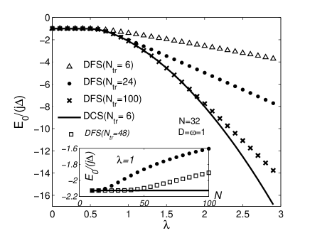
Figure 1: The scaled ground-state energy $E_{0}/(j\Delta)$ as a function of $\lambda$ by DCS and DFS with different truncated numbers. The inset show the scaled ground-state energy as a function of the $N$ for fixed $\lambda=1$.

To show the effectiveness of the present approach, we first calculate the ground-state energy $E_{0}$ by diagonalization in coherent-states (DCS) as described above , and compare with those by numerical diagonalization in Fock state (DFS) Emary for N=32. For convenience, we introduce two dimensionless parameters $D=\Delta/\omega$ and $\alpha=4\lambda^{2}/\Delta\omega$. Fig. 1 shows the scaled ground-state energy $E_{0}/(j\Delta)$ as a function of $\lambda$ when the Hamiltonain is on a scaled resonance $\Delta=\omega=1$ . For the same truncated number $N_{tr}=6$, the ground-state energy by DCS is much lower than that by DFS. With the increase of $N_{tr}$, DFS results approach the DCS one monotonously in the stronger coupling regime. One can find that the ground-state energy by DCS with $N_{tr}=6$ is even much better than that by DFS with $N_{tr}=100$. In addition, the DFS results become worse and worse as the N increases for fixed $N_{tr}$ and $\lambda$, as clearly shown in the inset of Fig. 1.

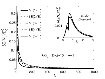
Figure 2: The relative ground-state energy difference as a function of $N$ for different truncated numbers $N_{tr}$ at critical point. The inset show $\delta E(N_{tr})$ as a function of $\lambda$ at fixed $N$ for different $N_{tr}$.

The ground-state energy is non-analytical at the critical point of the QPT in the thermodynamic limit. To show the effect of the precursor of the QPT on the present approach, we display the relative ground-state energy difference $\delta E(N_{tr})/E_{0}^{0}=(E_{0}^{N_{tr}}-E_{0}^{0})/E_{0}^{0}$ as function of $N$ at the critical point $\lambda_{c}$ in Fig. 2. It is interesting to find that as $N$ increases, the exact results can be obtained within smaller truncated number. This feature facilitates the calculation for rather large system size. In the inset of the Fig. 2, we can find that in both the weak and strong coupling regime, the results converge rapidly with the truncated number $N_{tr}$ for fixed large N, indicting that the Dicke model can be solved easily in these two limits. More interestingly, just in the critical regime, a dip structure is found in all curves, indicating a trace of QPT at finite size system.

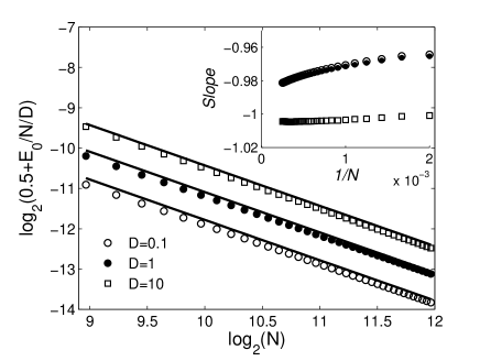
Figure 3: Scaling of the ground-state energy $E_{0}/ND+0.5$ as a function of $N$ at the critical point for $D=0.1,1$, and $10$. The inset show the corresponding slope versus $1/N$.

To study the universality of the QPT, we will compute the finite-size scaling exponents for several observables.

Ground-state energy.–We calculate the ground-state energy for different values of $D$. In the thermodynamical limit, $E_{0}/ND=-0.5$. We are able to study the system up to $N=2^{12}$ atoms in a PC. To show the leading finite-size corrections, we plot $E_{0}/ND+0.5$ versus $N$ for $D=0.1,1,10$ in a log-log scale in Fig. 3. The inset presents the slope as a function $1/N$. It is observed that the slope of all these curves in the large $N$ regime give a universal exponent $-1.0\pm 0.02$, from the above and below respectively, consistent with that by a modified Holstein-Primakoff approachvidal . The asymptotic behavior demonstrates that the exponent by no means lies on the vicinity of $-4/3$ in the the adiabatic regime reported in Ref. liberti .

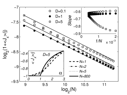
Figure 4: Scaling of the ground-state Berry phase $1+<J_{x}>/N$ as a function of $N$ at the critical point for $D=0.1,1$, and $5$. The upper inset show the corresponding slope as a function $1/N$, and the lower one gives the Berry phase versus $\alpha$ for different $N$ at $D=5$.

Berry phase.– To generate the Berry phase, we introduce a time-dependent unitary transformation $U(T)=exp[-i\phi(t)J_{x}]$, where $\phi(t)$ is changed adiabatically and slowly from $0$ to $2\pi$. The ground-state Berry phase can be defined asplastina

$$\gamma=i\int_{0}^{2\pi}<\varphi|U^{+}(t)\frac{d}{d\phi}U(t)|\varphi>d\phi=2\pi<\varphi|J_{x}|\varphi>$$ (8)

where $|\varphi>$ is just the time-independent ground-state wavefunction, which can be obtained by the present DCS. In the thermodynamical limit $<J_{x}>/N=-1$.

Fig. 4 shows the scaled ground-state Berry phase $1+<J_{x}>/N$ as a function of $N$ for different values of $D$ in log-log scale. A power law behavior exists in the large $N$. One can see from the upper inset that the finite-size exponents extracted from all curves tend to a converging value $(-0.67\pm 0.02)$. This result is in good agreement with that in Ref. (plastina ) with a adiabatic approximation. We find that the scaling exponent for the Berry phase in Dicke model is also universal, not merely in the adiabatic limit. The Berry phase tends to be discontinuous in the critical regime with the increase of $N$, shown in the lower inset.

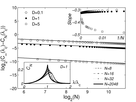
Figure 5: Scaling of concurrence as a function of $N$ at the critical point for $D=0.1,1$, and $5$. The upper inset show the slope versus $1/N$, the lower inset displays the scaled concurrence as a function of $\lambda/\lambda_{c}$.

Pairwise entanglement.–An important ground-state quantum essential feature is the concurrence, which quantifies the entanglement between two atoms in the atomic ensemble after tracing out over bosons. The scaled concurrence (entanglement) in the ground-state can be defined as $C_{N}=1-4<J_{y}^{2}>/N$ vidal ; wang . In the thermodynamic limit $N\rightarrow\infty$, the scaled concurrence at critical point $C_{\infty}(\lambda_{c})$ can be determined in terms of $D$ Lambert2 . For comparison, we can calculate the quantity $C_{\infty}(\lambda_{c})-C_{N}(\lambda_{c})$. In Fig. 5, we present this quantity as a function of $N$ for different values of $D$ in log-log scale. Derivative of these curves is presented in the upper inset, and the exponent of concurrence is estimated to be ${-0.33\pm 0.02}$. For large $D$, the exponent for concurrence is only given reasonably in the asymptotic regime. From the lower inset, we find that a cusp is formed with increasing $N$ in the critical regime, demonstrating the relic of the QPT in finite size.

Lambert et al., performed a numerical DFS and give the exponent of concurrence ${-0.25\pm 0.01}$ Lambert2 with $N\leq 32$. Reslen et al., derived a effective Hamiltonian, and found the exponent to be ${-0.26\pm 0.02}$ with $N\leq 35$.reslen Recently, Vidal et al. using the diagonalizing a expanded Hamiltonian at order $1/N$ based on Holstein-Primakoff representation, and predicted finite-size scaling exponent for concurrence $1/3$ vidal , agreeing well with our results. Due to the huge system size we can touch here, the previous controversy can be attributed to the small system size Lambert2 ; reslen .

In summary, we have proposed a numerically exact solution to the Dicke model in the whole coupling regime for a huge system size up to $N=2000\thicksim 4000$, which is almost two orders of magnitude higher than that reported in literature Lambert2 ; reslen . Several quantities related to QPT such as the ground-state energy, the Berry phase, and the concurrence are then calculated exactly. It is found that the scaling exponent for the ground-state energy is different from that in a previous studyliberti . The previous discrepancy for the exponent of concurrence is reconciled by the present calculation in very large size systems. The precise estimate of the scaling exponent for these quantities is very significant to clarify the universality of QPT. The methodology sketched here is helpful to study a large number of spin(fermion)-boson coupling systems.

This work was supported by National Natural Science Foundation of China, PCSIRT (Grant No. IRT0754) in University in China, and National Basic Research Program of China (Grant No. 2009CB929104).

References

- (1) R. H. Dicke, Phys. Rev. 93, 99(1954).
- (2) S. Sachdev, Quantum Phase Transitions (Cambridge University Press, Cambridge, England, 2000).
- (3) K. Hepp and E. Lieb, Ann. Phys., 76, 360(1973).
- (4) A. Osterloh, L. Amico, G. Falci, and R. Fazio, Nature (London) 416, 608(2002); T. J. Osborne and M. A. Nielsen, Phys. Rev. A. 66, 032110(2002); S. J. Gu, H. Q. Lin, and Y. Q. Li, ibid. 68, 042330(2003).
- (5) A. C. M. Carollo and J. K. Pachos, Phys. Rev. Lett. 95, 157203(2005); S.- L. Zhu, Phys. Rev. Lett. 96, 077206(2006).
- (6) C. Emary and T. Brandes, Phys. Rev. E 67, 066203(2003); Phys. Rev. Lett. 90, 044101(2003).
- (7) N. Lambert, C. Emary, and T. Brandes, Phys. Rev. A. 71, 053804(2005).
- (8) V. Buzek, M. Orszag, and M. Rosko, Phys. Rev. Lett. 94, 163601(2005).
- (9) N. Lambert, C. Emary, and T. Brandes, Phys. Rev. Lett. 92, 073602(2004).
- (10) G. Liberti, F. Plastina, and F. Piperno, Phys. Rev. A 74, 022324 (2006).
- (11) J. Vidal and S. Dusuel, Europhys. Lett. 74, 817(2006).
- (12) J. Reslen, L. Quiroga, and N. F. Johnson, Europhys. Lett. 69, 8(2005).
- (13) F. Plastina, G. Liberti, and A. Carollo, Europhys. Lett. 76, 182(2006).
- (14) M. Scheibner et al., Nature Phys. 3, 106(2007).
- (15) D. Schneble et al., Science 300, 475 (2003).
- (16) M. J. Hartmann et al., Nature Phys. 2, 849(2006); A. D. Greentree et al., ibid. 2, 856(2006).
- (17) A. Wallraff et al., Nature (London) 431, 162 (2004);R. W. Simmonds et al., Phys. Rev. Lett. 93, 077003(2005).
- (18) Y. Yu et al., Science 296, 889 (2002); I. Chiorescu et al., Science 299, 1869 (2003).
- (19) Q. H. Chen et al., Phys. Rev. B 53, 11296(1996).
- (20) R. S. Han, Z. J. Lin, and K. L. Wang, Phys. Rev. B 65, 174303(2002)
- (21) K. L. Wang, T. Liu, and M. Feng, Euro. Phys. J. B 54, 283(2006).
- (22) G. S. Tian, L. H. Tang, and Q. H. Chen, Europhys. Lett. 50, 361(2000); Phys. Rev. B63, 054511(2001).
- (23) X. Wang, K.Mølmer, Eur. Phys J. D 18, 385(2002).