Polarized thermal emission by thin metal wires

Abstract

We report new measurements of the linear polarization of thermal radiation emitted by incandescent thin tungsten wires, with thicknesses ranging from five to hundred microns. Our data show very good agreement with theoretical predictions, based on Drude-type fits to measured optical properties of tungsten.

1 Introduction

Thermal radiation by incandescent bodies has been the subject of intense theoretical and experimental investigations for over a century now. While the laws of thermal emission by a blackbody are at the very roots of Quantum Theory [1], the richness of phenomena involved in thermal emission has been fully realized only quite recently. Perhaps, the most interesting progress has been the realization that thermal radiation may exhibit a significant degree of spatial and temporal coherence, in seeming contradiction with one’s idea that thermal emission is an incoherent phenomenon. Among the most recent findings, we mention as an example the remarkable degree of spatial coherence of the radiation of a hot body in the near-field region [2]. Coherence features of thermal radiation are also at the basis of recent attempts to modify or tailor the profile of thermal emission by metallodielectric surfaces, with subwavelength patterns, that are of great importance in applied physics and engineering (see Refs.[3, 4, 5, 6, 7, 8] and references therein).

Another striking example of this sort was discovered quite some time ago by $\ddot{\rm O}$hman [9], who observed that visible radiation from a hot thin metallic wire shows a significant polarization. Using incandescent tungsten filaments with a thickness of a few microns, this author found a polarization in the direction orthogonal to the wire as high as 28 per cent, in the red region of the spectrum. In a related attempt to explain these preliminary findings, Agdur et al. [10] investigated in detail the scattering and absorption of light by thin metal wires, using silver wires having a diameter down to 2000 Å. The data were compared with a simple theoretical model, where the ”plasma” properties of the metal were taken into account, showing good agreement with the measurements. Even though scattering and absorption data are related theoretically, via Kirchhoff’s law, to thermal emission, the authors of Ref.[10] could not perform accurate measurements of the degree of polarization of the radiation emitted by the wires, due to technical difficulties, and only report that a polarization of about fifty per cent was found in the case of silver filaments with a diameter of about 0.8 microns.

After these early findings, several authors have recently investigated the polarization features of the thermal radiation emitted by a number of sources with different designs, like platinum microwires [5, 8], semiconductor layers placed in an external magnetic field [11], SiC lamellar gratings [12]. In this paper, we report new measurements of the ”linear polarization” (see Sec. 2) of thermal radiation emitted by individual incandescent tungsten wires, with thicknesses between five and hundred microns. Our work is closely related to Refs.[5, 8], which report measurements of the polarization and angular distribution of thermal radiation from individual antenna-like, thin film platinum microwires, heated at a temperature of 900 K. While the quantity that we measure to characterize the polarization of the thermal radiation is essentially the same as the ”extinction ratio $E$” measured in [5, 8], two differences between our work and Refs.[5, 8] should be stressed. Apart from the fact that we use tungsten instead of platinum, which allows us to work in the visible region of the spectrum, the main difference is in the relative magnitude of the wires thickness, as compared to the wavelength of the observed radiation. While the lateral extent of the microwires of Refs. [5, 8] is in fact smaller than (or comparable to) the wavelengths of the infrared radiation observed there, we are quite in the opposite situation, since our wires are always much thicker than the wavelengths that we observe. As it will be seen in greater detail in the next Section, the polarization features of the thermal radiation are quite opposite in the two regimes: while for very thin wires, as reported in [5, 8], the thermal radiation is polarized in a direction parallel to the wire, in the case of thicker wires the situation is reversed, and the radiation is now polarized in the direction orthogonal to the wire, the crossover occurring for wavelengths roughly equal to the circumference of the wire. This latter case is the one originally reported in Ref. [9], and it is the one explored in the present paper.

The paper is organized as follows: in section 2 we derive the theoretical expression for the linear polarization of thermal emission by a wire. In section 3 we describe our apparatus and present our measurements, while in section 4 the experimental data are compared with theoretical predictions. In Section 5 we draw our conclusions, and finally in the Appendix we present the detailed expression of the Drude-type fit to the optical data of tungsten, as given in Ref.[13], that we used for our numerical computations.

2 Theory

2.1 General equations

We model the wire as a homogeneous circular cylinder ${\cal C}$ of length $l$ and radius $a$. The observation point is placed at a distance $r$ from the wire, in the plane passing trough the mid point of the wire and orthogonal to it. It is further assumed that $a$, $l$ and $r$ satisfy the conditions

$$a^{2}\ll\lambda\,r\ll l^{2}\;,$$ (1)

where $\lambda$ is the wavelength of radiation. Under this assumption, the radiation field at the observation point coincides with the far-field for an infinitely long cylinder. The material constituting the wire is described as a homogenous dielectric with a complex permittivity $\epsilon(\omega)$ depending on the frequency $\omega$, and obviously on the temperature $T$ of the wire. As we consider non-magnetic materials, we shall set to one the magnetic permeability $\mu$.

Cylindrical symmetry of the system permits to introduce TE and TM modes of the electromagnetic field [14]: TE modes have their electric field ${\bf E}$ in the plane orthogonal to the cylinder axis, which we take to coincide with the $z$ direction. On the contrary, TM modes have their magnetic field ${\bf B}$ orthogonal to the cylinder axis. At large distances from the wire, the electric field is orthogonal to the line of sight, and for TE modes it is orthogonal to the wire, while for TM modes it is parallel to it. The $z$-components of the electric and magnetic fields, $E_{z}$ and $B_{z}$, can be taken as independent fields, from which all other components of ${\bf E}$ and ${\bf B}$ can be obtained using Maxwell equations. TE modes are then characterized by the condition $E_{z}^{({\rm TE})}=0$, while for TM modes we have $B_{z}^{({\rm TM})}=0$. Therefore TE and TM modes are labelled by $B_{z}$ and $E_{z}$, respectively. Outside ${\cal C}$, both $B_{z}$ and $E_{z}$ satisfy the Helmholtz equation:

$$-(\nabla^{2}+k^{2})E_{z}=-(\nabla^{2}+k^{2})B_{z}=0\,,$$ (2)

where $k=\omega/c$. We collect $B_{z}$ and $E_{z}$ in a two-dimensional vector ${\bf u}$:

$${\bf u}\equiv\left(\begin{array}[]{c}B_{z}\\ E_{z}\\ \end{array}\right)\,.$$ (3)

Since we only observe radiation that is emitted in a narrow solid angle around a direction orthogonal to the $z$ axis, we can just consider fields that propagate in the $(x,y)$ plane and are thus independent of the $z$-coordinate. For normal incidence, TE and TM modes do not mix under scattering by the wire and therefore, outside ${\cal C}$, ${\bf u}$ is a superposition of partial waves ${u}_{m}^{(\alpha)}$ with definite polarization $\alpha$ and angular momentum $m$ along the $z$-axis:

$${u}_{m}^{(\alpha)}=\left(\,H_{m}^{(2)}(k\,r)+{{\cal S}}_{m}^{(\alpha)}(k)\,H^{(1)}(k\,r)\right)e^{im\phi}\,,$$ (4)

where $\phi$ is the azimuthal angle, and $H^{(i)}$ are Hankel functions. The scattering amplitudes ${{\cal S}}_{m}^{(\alpha)}(k)$ measure the response of the wire to a unit amplitude incoming wave with wave-vector $k$, polarization ${\alpha}$ and angular momentum $m$ along the wire. It should be noted that, with the wire absent, ${{\cal S}}_{m}^{(\alpha)}(k)\rightarrow 1$, and then the partial waves ${u}_{m}^{(\alpha)}$ would reduce to $2\,J_{m}(k\,r)\exp(im\phi)$, the partial wave solution regular along the $z$-axis.

By use of Kirchhoff’s law, one easily finds that the emissivity $e^{(\alpha)}(k)$ of the wire for polarization $\alpha$ is:

$$e^{(\alpha)}(k)=\sum_{m=-\infty}^{\infty}(1-|{{\cal S}}_{m}^{(\alpha)}(k)|^{2})\;.$$ (5)

It is convenient to reexpress the above formula for the emissivity in terms of the so-called transition amplitudes ${\cal T}_{m}^{(\alpha)}(k)$ defined as:

$${\cal T}_{m}^{(\alpha)}(k)=\frac{1}{2}(1-{\cal S}_{m}^{(\alpha)}(k))\;.$$ (6)

We then obtain:

$$e^{(\alpha)}(k)=4\sum_{m=-\infty}^{\infty}[\,{\rm Re}({\cal T}_{m}^{(\alpha)}(k))-|{{\cal T}}_{m}^{(\alpha)}(k)|^{2})\,]\,.$$ (7)

The explicit expressions for the transition amplitudes ${\cal T}_{m}^{(\alpha)}(k)$ can be easily obtained by solving the scattering problem for a homogeneous dielectric cylinder [14]. The result is:

$${\cal T}_{m}^{({\rm TE})}(k)=\frac{J^{\prime}_{m}(nka)\,J_{m}(ka)-n\,J^{\prime}_{m}(ka)\,J_{m}(nka)}{J^{\prime}_{m}(nka)\,H_{m}^{(1)}(ka)-n\,J_{m}(nka)\,H_{m}^{(1)\,^{\prime}}(ka)}\,,$$ (8)

$${\cal T}_{m}^{({\rm TM})}(k)=\frac{J_{m}(nka)\,J_{m}^{\prime}(ka)-n\,J^{\prime}_{m}(nka)\,J_{m}(ka)}{J_{m}(nka)\,H_{m}^{(1)\,^{\prime}}(ka)-n\,J^{\prime}_{m}(nka)\,H_{m}^{(1)}(ka)}\,.$$ (9)

In the above formulae, a prime denotes differentiation, while $n=\sqrt{\epsilon}$ is the (complex) refraction index. Following the terminology of Ref.[15], we define the linear polarization $P(k)$ of the thermal emission of the wire by the formula:

$$P(k)=\frac{e^{({\rm TE})}(k)-e^{({\rm TM})}(k)}{e^{({\rm TE})}(k)+e^{({\rm TM})}(k)}\,$$ (10)

with the positive sign corresponding to polarization in the direction orthogonal to the wire. The quantity $P(k)$ above is the observable considered in Refs.[9, 10] and it is basically the same as the extinction ratio $E$ considered in Refs.[5, 8] ($P=-E/(2+E)$). We should remark that the quantity $P$ does not provide a complete characterization of the degree of polarization of the radiation, which is properly described in terms of the Stokes parameters [16]. A complete determination of the Stokes parameters requires observation of the circular polarization of the emitted radiation, but unfortunately our apparatus does not permit it. We therefore content ourselves with the partial information contained in the linear polarization $P$ above. In Figure 1 we plot the theoretical prediction for $P$ as given by Eq. (10), for a tungsten wire, as a function of $\log(2\pi a/\lambda)$, for $\lambda=.5\;\mu$m. The curve was computed using the Drude-like fit to the optical data for tungsten quoted in Ref.[13], for a wire temperature $T=2400$ K (see Appendix for details). The most striking feature seen in Figure 1 is the change of sign of $P$ that occurs as the thickness of the wire is decreased: while for thick wires the radiation is polarized in the direction orthogonal to the wire, for wires having a thickness (or better to say a circumference $2\,\pi\,a$) comparable to or smaller than the wavelength $\lambda$, the axis of polarization aligns with the wire. We remark that the former behavior is the one reported for the first time in [9, 10], while the latter one was observed recently in [5, 8] using very thin platinum microwires. Another remarkable feature of $P$ as a function of $a$ is not clearly visible from Figure 1, and can be better seen from Figure 4 below: in the thick wire regime, $P$ is not a monotonically increasing function of $a$, and it displays a maximum for a definite value of $a$. We have not been able to find a simple explanation of this feature of the curve.

The quantity that we actually measure really is an average $\mathbb{P}$ of $P(k)$ over the wavelengths that get through a polarizing filter placed between the wire and the detector. The transmission efficiency of the filter is characterized by a transmission coefficient $\chi(\lambda)$, comprised between zero (no transmission) and one (full transmission). The average linear polarization $\mathbb{P}$ can then be written as:

$$\mathbb{P}=\frac{{\bar{e}}^{({\rm TE})}-{\bar{e}}^{({\rm TM})}}{{\bar{e}}^{({\rm TE})}+{\bar{e}}^{({\rm TM})}}\,,$$ (11)

where

$${\bar{e}}^{(\alpha)}=\frac{1}{N}\int_{0}^{\infty}d\lambda\,\chi(\lambda)\,E(\lambda,T)\,e^{(\alpha)}(2\pi/\lambda)\;.$$ (12)

In this equation, $E(\lambda)$ is Planck formula (expressed in terms of the wavelength $\lambda$):

$$E(\lambda,T)=\frac{2\pi h\,c^{2}}{\lambda^{5}}\frac{1}{e^{\lambda_{T}/\lambda}-1}\;,$$ (13)

where $\lambda_{T}=hc/(k_{B}T)$, and $N$ is a normalization constant $N=\int_{0}^{\infty}d\lambda\chi(\lambda)E(\lambda,T)$.

Figure 1: Plot of the linear polarization $P$ (see text for explanation) for a tungsten wire of radius $a$, versus $\log(2\pi a/\lambda)$. The curve is computed for a fixed wavelength $\lambda=.5\,\mu$m, using the Drude-like fit to the optical data of tungsten for $T=2400$ K (see Appendix).

2.2 The limit of thick wires

In the limit of thick wires, $a\gg\lambda$, it is possible to derive a very simple expression for the linear polarization $P$ of the radiation emitted by the wire in a direction orthogonal to $z$ [17]. When $a\gg\lambda$, diffraction effects become negligible, and we can regard the surface of the wire as locally flat. Let us say, for definiteness, that the line of sight coincides with the $x$ direction. Then, the emissivity of the wire in the direction $x$, for polarization $\alpha$, is easily found to be:

$$e^{(\alpha)}(k)=\frac{1}{2}\int_{-\pi/2}^{\pi/2}d\phi\cos(\phi)\;e^{(\alpha)}_{\rm plane}(k,\phi)\,,$$ (14)

where $e^{(\alpha)}_{\rm plane}(k,\phi)$ is the emissivity for a flat surface made of the same material, in the direction forming an angle $\phi$ with the normal to the plane. On the other hand, from Kirchhoff’s law we have:

$$e^{(\alpha)}_{\rm plane}(k,\phi)=1-|R^{(\alpha)}(k,\phi)|^{2}\,,$$ (15)

where $R^{(\alpha)}(k,\phi)$ are the familiar Fresnel reflection coefficients for radiation incident at an angle $\phi$. Using Eqs. (14) and (15) in the expression of $P$, Eq. (10), we obtain:

$$P\simeq\frac{\int_{-\pi/2}^{\pi/2}d\phi\,\cos\phi\,(|R^{({\rm TE})}(k,\phi)|^{2}-|R^{({\rm TM})}(k,\phi)|^{2})}{\int_{-\pi/2}^{\pi/2}d\phi\,\cos\phi\,(2-|R^{({\rm TE})}(k,\phi)|^{2}-|R^{({\rm TM})}(k,\phi)|^{2})}\;.$$ (16)

With our choices of polarization, the explicit expressions for $R^{(\alpha)}(k,\phi)$ are:

$$R^{({\rm TE})}(k,\phi)=\frac{\epsilon\cos\phi-\sqrt{\epsilon-1+\cos^{2}\phi}}{\epsilon\cos\phi+\sqrt{\epsilon-1+\cos^{2}\phi}}\;,$$ (17)

$$R^{({\rm TM})}(k,\phi)=\frac{\cos\phi-\sqrt{\epsilon-1+\cos^{2}\phi}}{\cos\phi+\sqrt{\epsilon-1+\cos^{2}\phi}}\;.$$ (18)

3 Experiments

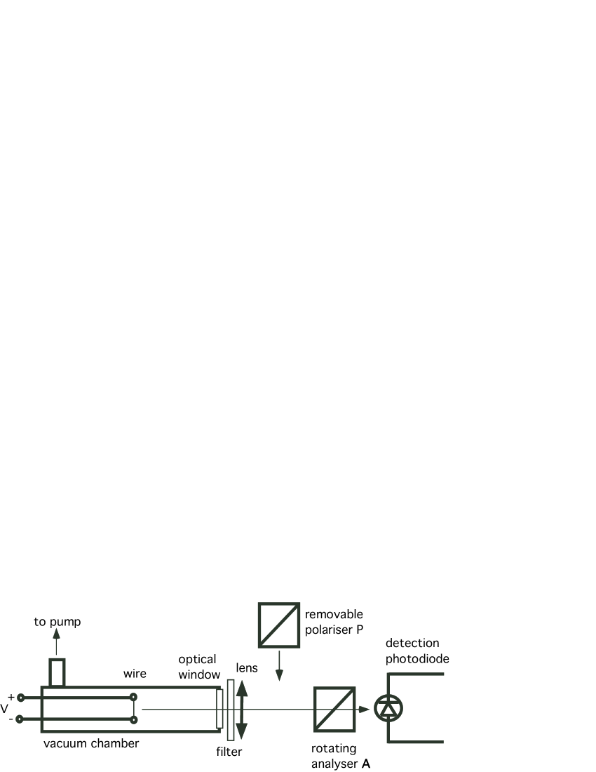
Figure 2: Drawing (not to scale) of the experimental apparatus.

The experimental apparatus (see figure 2) consists of a vacuum cylindrical chamber in which the metal wire is positioned perpendicular to the chamber axis. The chamber is 52 cm long and has a 2.5 cm diameter, and a pumping system provides a working residual pressure about $10^{-6}$ mbar. The 7 mm long wire is sustained by two electrical feedthroughs providing the flowing current to set the wire incandescent. An optical window allow for light emitted by the wire to exit from the vacuum region. The tube internal surface is mat and painted with aquadag in order to prevent reflections: this way, light emerges from the tube roughly parallel to its axis. This light, after passing a bandpass filter is imagined onto a detection photodiode by a lens. In order to study the polarization properties of emitted light, a pair of polaroid polarizers have been used. These polarizers (Edmund Optics TECHSPEC) work only in a limited bandwidth centered in the visible domain. Since light emitted from the wire lies mainly in the infrared spectral region, the bandpass filter (Thorlabs model FES750) selects light in the spectral band from 450 to 750 nm. In order to avoid systematics due to residual infrared light impinging on the photodiode, the following procedure has been used.

Step 1. The rotating analyser A is placed on the optical path. Measurements are taken rotating the analyser and recording the photodiode signal every 0.5 degree. The light intensity on the photodiode can be written as:

$$I_{1}=A_{1}\cos^{2}(\theta-\theta^{*})+F_{1}\;,$$ (19)

where $\theta$ is the angular position of the analyser, $A_{1}$ measures the maximum amount of polarized light impinging on the photodiode and $F_{1}$ is the sum of unpolarized light and of the residual infrared light. Due to this residual, this single measurement is not sufficient to determine the linear polarization, which is given by:

$$\mathbb{P}=\frac{I_{P}}{I_{P}+I_{U}}\;,$$ (20)

where $I_{P}$ and $I_{U}$ refer to the intensities of linearly polarized and unpolarized light emitted by the filament. The purpose of this step 1 is to determine the angle $\theta^{*}$ of maximum transmission for the emitted light (Electric field), which corresponds to the maximum for $I_{1}$.

Step 2. Insert the polarizer P in the optical path. Two sets of measurements are taken with the analyser, for the two directions of the polariser P as $\theta^{*}$ and $\theta^{*}+\frac{\pi}{2}$.

$$I_{2}^{a} = A_{a}\cos^{2}(\theta-\theta_{a})+F_{2}\,\,\,\,\,\,\,\,({\rm{\bf P}\,\,set\,\,to\,\,}\theta^{*})$$ (21)

$$I_{2}^{b} = A_{b}\cos^{2}(\theta-\theta_{b})+F_{2}\,\,\,\,\,\,\,\,({\rm{\bf P}\,\,set\,\,to\,\,}\theta^{*}+\frac{\pi}{2})\;.$$ (22)

Now $F_{2}$ has only the infrared residual, while $A_{a}$ is proportional to $I_{P}$ plus half the unpolarized light $I_{U}/2$ and $A_{b}$ only to $I_{U}/2.$ It follows then:

$$\mathbb{P}=\frac{A_{a}-A_{b}}{A_{a}+A_{b}}\;.$$ (23)

Collected data are fitted using least square analysis. This allows a precise determination of the coefficients $A_{i}$ and a control of the correct positioning of the polarimeter P: in all the measurements the discrepancy between the angles $\theta_{a},\theta_{b}$ and $\theta^{*},\theta^{*}+\frac{\pi}{2}$, was kept below 0.5 degree.

Measurements have been performed using four pure tungsten wires provided by LUMA Metall, with diameter 5, 17, 35 and 100 $\mu$m. For each wire three different values of voltage were applied to the feedthroughs, to check for possible changes of the degree of polarization with temperature. To get a rough estimate of the temperature two different methods have been used: in the first the resistivity is calculated and compared to tabulated values. In the second, temperature is deduced by the assumption that the total electrical power is converted into radiation. The computed values are affected by large errors, mainly due to the fact that temperature is not uniform along the wire, but rather follows a sort of flat top profile. This can be seen for example from the picture of Figure 3. The estimates for the temperature show that values are in the range 2600 - 3200 K. For all the wires a range of temperature of 300 – 400 K is spanned by varying the voltage.

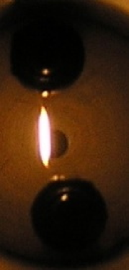
Figure 3: A photograph of the 5 $\mu$m diameter wire with 10 mA current flowing through it. The two black circles on the upper and lower ends are the feedthroughs.

Table 1: Summary of the measurements.

diameter ($\mu$m)	voltage (V)	current (A)	$\mathbb{P}$	avg($\mathbb{P}$)
5	2.5	8.8 10-3	0.2416	0.241 $\pm$ 0.005
	3.0	9.6 10-3	0.2353
	3.9	10.9 10-3	0.2446
17	1.7	9.6 10-2	0.2179	0.221 $\pm$ 0.003
	2.0	0.106	0.2237
	2.4	0.117	0.2219
35	1.1	0.309	0.2119	0.208 $\pm$ 0.003
	1.2	0.32	0.2059
	1.4	0.343	0.2078
100	2.0	1.81	0.2028	0.199 $\pm$ 0.004
	2.3	1.96	0.1956
	2.45	1.98	0.1981

Table 1 lists the obtained results. Measurements accuracy affects the determination of each value of $\mathbb{P}$ in a negligible manner: the largest absolute error resulting 0.001 (relative error less than 0.5 %), much smaller than the spread of the values for each single wire. The average value has then been taken as the arithmetic mean with the error the standard deviation. The polarization direction (Electric field) has been found orthogonal to the wire for all measurements.

4 Comparison with theory

For the purpose of comparing our data with the theoretical value of $\mathbb{P}$, the following choices were made. We approximated the transmission coefficient $\chi(\lambda)$ of the polarizer by a stepwise constant function, as follows:

$$\chi(\lambda)=\left\{\begin{array}[]{c}0\;\;\;\;\;{\rm for}\;\lambda<\lambda_{1}\\ \;\;\;\;\;\;\;1\;\;\;\;{\rm for}\;\lambda_{1}<\lambda<\lambda_{2}\\ 0\;\;\;\;\;{\rm for}\;\lambda>\lambda_{2}\\ \end{array}\right.$$ (24)

and we took $\lambda_{1}=0.5$ micron and $\lambda_{2}=0.75$ micron. This crude model describes sufficiently well the actual transmission coefficient of the filter we used. For the complex dielectric function $\epsilon(\omega)$ we used the Drude-type analytical fits to optical data of tungsten quoted in Ref.[13] (see Appendix for details). This reference provides the permittivity of tungsten for several temperatures in the range from 298 K to 2400 K. Unfortunately, no data are reported for temperatures higher than 2400 K, as it is the case in our measurements. We remark that the formulae reported in Ref.[13] contain no adjustable free parameters. In Figure 4, we show our experimental data for three different thicknesses (full diamonds with error bars) together with the plots of three theoretical curves for $\mathbb{P}$ as a function of the wire diameter (in microns). The theoretical curves have been computed for three different temperatures, $T=298$ K, $T=1600$ K and $T=2400$ K. We can see clearly that the theoretical curve computed using room-temperature optical data is definitely not consistent with our measurements, while already the curve for 2400 K fits the data rather well. Since the three theoretical curves show that the polarization decreases by increasing temperature, it is likely that an even better agreement with the data would have resulted, had we had at our disposal data for the permittivity relative to temperatures around 2600-3200 K, or so, which we expect to be the range of temperatures reached by our wires.

Figure 4: Experimental data (diamonds with error bars) and theoretical curves for the average linear polarization. The wire diameter along the $x$-axis is in microns. The three theoretical curves displayed have been computed using the Drude-like fits (with no free parameters) reported in [13] to optical data of tungsten for three different temperatures: the solid line is for $T=2400$ K, the dotted line is for $T=1600$ K, the dot-dashed line is for $T=298$ K.

In Table 2 we quote the detailed experimental data, and the theoretical prediction for $T=2400$ K.

diameter ($\mu$m)	5	17	35	100
$\mathbb{P}_{\rm exp}$	0.241$\pm$0.005	0.221$\pm$0.003	0.208$\pm$0.003	0.199$\pm$0.004
$\mathbb{P}_{\rm theor}$	0.2435	0.222	0.209	0.20

Table 2: Experimental and theoretical values of the linear polarization. The theoretical values are computed using optical data for $T=2400$ K.

5 Conclusions

The fact, contrary to one’s intuition of thermal phenomena, that thermal radiation from incandescent bodies may reveal unexpected coherent features is nowadays well appreciated. A remarkable example of this sort is the polarization of the radiation emitted by a thin incandescent wire, in the direction orthogonal to the wire, that was reported for the first time by $\ddot{\rm O}$hman long ago [9]. These initial findings were later confirmed in a preliminary series of measurements by Agdur et al.[10] with platinum filaments having thicknesses between one and ten microns. These authors observed an increasing linear polarization with decreasing thicknesses and a maximum polarization of about fifty percent. However, the insufficient quality of the measurements did not allow for a rigorous comparison between theory and experiment. In this paper we have reported new measurements of the linear polarization of thermal radiation emitted by incandescent thin tungsten wires, with thicknesses ranging from five to hundred microns, and temperatures in the interval from 2600 to 3200 K. For thicknesses in this range we observe an increasing linear polarization with decreasing thickness, in qualitative agreement with the results of [10]. We have compared our measurements with theoretical predictions, based on the available optical data for tungsten [13], referring to filaments with temperatures ranging from 298 K to 2400 K, and we found very good agreement between our measurements and the theoretical prediction derived from the 2400 K data. Interestingly enough, for small wire thicknesses, theory predicts an inversion of the qualitative dependence of the linear polarization with wire thickness. As it can be seen from Fig. 4, we note that for thicknesses smaller than about four microns, a decrease of thickness is expected to engender a smaller polarization, contrary to the behavior predicted (and observed by us) for thicker wires. Unfortunately, we could not perform any measurements with wires thinner than five microns, in order to observe this interesting inversion phenomenon.

6 Appendix

The optical properties of tungsten, in the wavelength range from 0.365 to 2.65 microns, were measured long ago by Roberts [13]. He showed that the following formula for the permittivity $\epsilon$, adapted from Drude’s well known expression, adequately fits the data:

$$\epsilon=1+\sum_{p}\frac{K_{0p}\lambda^{2}}{\lambda^{2}-\lambda_{sp}^{2}+i\delta_{p}\lambda_{sp}\lambda}\,-\,\frac{\lambda^{2}}{2\pi c\epsilon_{0}}\sum_{q}\frac{\sigma_{q}}{\lambda_{rq}-i\lambda}\,,$$ (25)

where $\lambda$ is the wavelength in vacuum, $c$ is the velocity of light and $\epsilon_{0}$ is the permittivity of vacuum (in mks units). The first sum in the r.h.s. of Eq. (25) represents a bound-electrons contribution, while the second sum is a free-electron contribution. If the above equation is extrapolated to very low frequencies, one obtains the limiting value $\sigma_{0}=\sum_{q}\sigma_{q}$ for the dc conductivity. For convenience of the reader, the numerical values of the parameters for a number of temperatures, as quoted in [13], are reproduced in Table 3. The bound-electron contribution at the higher temperatures is substantially the same as that at 1600 K, and for this reason the corresponding parameters $K_{0p},\lambda_{sp}$ and $\delta_{p}$ are not displayed in the last two columns of Table 3.

Temp.	298 K	1100 K	1600 K	2000 K	2400 K
$\sigma_{1}$	17.50	3.50	2.14	(1.58)	(1.19)
$\sigma_{2}$	(0.21)	0.16	0.19	(0.22)	(0.25)
$\lambda_{r1}$	45.5	9.3	6.0	(4.63)	(3.66)
$\lambda_{r2}$	(3.7)	$<0.36$	$<0.36$	$(<0.36)$	$(<0.36)$
$K_{01}$	12.0	10.9	10.9
$K_{02}$	14.4	13.4	13.4
$K_{03}$	12.9	12.0	12.0
$\lambda_{s1}$	1.26	1.40	1.40
$\lambda_{s2}$	0.60	0.57	0.57
$\lambda_{s3}$	0.30	0.25	0.25
$\delta_{1}$	0.6	1.0	1.0
$\delta_{2}$	0.8	1.2	1.2
$\delta_{3}$	0.6	1.0	1.0
$\sigma_{1}/\lambda_{r1}$	0.385	0.376	0.357	(0.341)	(0.325)
$\sigma_{0}$	17.7	3.67	2.34	1.80	1.44

Table 3: Optical data for tungsten from [13]. $(\;)$ indicates tentative estimates. Conductivities ($\sigma_{1}$, etc.) are in units of $10^{6}$ ohm^-1m^-1. The dc conductivity is $\sigma_{0}$. Wavelengths ($\lambda_{r1}$, etc.) are in microns.

References

References

- [1] Planck M 1901 Ann. Phys. 4 553
- [2] Carminati R and Greffet J J 1999 Phys. Rev. Lett. 82 1660
- [3] Laroche M, Arnold C, Marquier F, Carminati R and Greffet J J, 2005 Opt. Lett. 30 2623
- [4] Chan D L C, Soljai M and Joannopoulos J D 2006 Phys. Rev. E 74 016609
- [5] Ingvarsson S, Klein J L, Au Y Y, Lacey J A and Hamann H F 2007 Opt. Expr. 15 11249
- [6] Dahan N, Niv A, Biener G, Gorodetski Y, Kleiner V and Hasman E 2007 Phys. Rev. B 76 045427
- [7] Biener G, Dahan N, Niv A, Kleiner V and Hasman E 2008 App. Phys. Lett. 92 081913
- [8] Au Y Y, Skulason H S, Ingvarsson S, Klein J L and Hamann H F 2008 Phys. Rev. B 78 085402
- [9] hman Y 1961 Nature 192 254
- [10] Adgur B, Bling G, Sellberg F and hman Y 1963 Phys. Rev. 130 996
- [11] Kollyukh O G, Liptuga A I, Morozhenko V, Pipa V I and Venger E F 2007 Opt. Commun. 276 131
- [12] Marquier F, Arnold C, Laroche M, Greffet J J and Chen Y 2008 Opt. Expr. 16 5305
- [13] Roberts S 1959 Phys. Rev. 114 104
- [14] Jackson J D 1999 Classical Electrodynamics (New York: Wiley)
- [15] Smith G S (2007) Am. J. Phys. 75 25
- [16] Born M and Wolf E 2003 Principles of Optics (Cambridge University Press)
- [17] Bertilone D C 1994 J. Opt. Soc. Am. A 11 2298