Electron-phonon bound states and impurity band formation in quantum wells

Abstract

A generalized propagation matrix method is used to study how scattering off local Einstein phonons affects resonant electron transmission through quantum wells. In particular, the parity and the number of the phonon mediated satellite resonances are found to depend on the available scattering channels. For a large number of phonon channels, the formation of low-energy impurity bands is observed. Furthermore, an effective theory is developed which accurately describes the phonon generated sidebands for sufficiently small electron-phonon coupling. Finally, the current-voltage characteristics caused by phonon assisted transmission satellites are discussed for a specific double barrier geometry.

I Introduction

Resonant tunneling through quantum wells has been extensively studied in semiconductor heterostructures, such as $\rm GaAs/Al_{x}Ga_{1-x}As$ double barriers goldman87 ; boebinger90 ; chen91 ; geim94 ; kim03 . More recently, analogous electron transmission processes have also been investigated in the context of molecular junctions nitzan03 ; benesch06 ; mitra04 ; braig03 ; galperin07 and mesoscopic rings yacoby95 ; buks96 . Resonant tunneling is a purely quantum effect whereby electrons pass through structures made of potential wells and barriers with unit or near-unit transmission probabilities if they enter the quantum well at the particular energies of the structure’s bound states. Following the initial experimental observation of satellite peaks of these transmission resonances goldman87 , a large volume of theoretical work levi89 ; cai89 ; cai90 ; cai91 ; wu91 ; stovneng91 ; bagwell92 ; grein93 ; zhou93 ; bonca95 ; bonca97 ; haule99 ; mohaidat93 ; brandes02 has focused on the effects of phonon scattering on the electronic tunneling. Early on, it was recognized that perturbative treatments tend to miss the essential feedback effects between elastic and inelastic channels which lead to these satellite features in the electronic transmission levi89 . In particular, it was found that electron-phonon scattering processes can cause the formation of polaronic bound states, leading to phonon assisted resonant tunneling cai89 ; cai90 ; cai91 ; wu91 . More recent works have shown that within a tight-binding description these features are further enhanced stovneng91 , and phonon bands can form bonca95 ; bonca97 . Furthermore, theoretical models have been generalized to include the effects of the three-dimensional environment bagwell92 ; zhou93 , non-equilibrium dynamics grein93 , and finite temperatures haule99 .

In this paper, we examine the hierarchy of polaronic resonances in the electron transmission through quantum well structures. In particular, we focus on even-odd effects with respect to the number of available phonon channels and on the emergence of impurity bands as this number becomes large. We also apply an effective theory which reproduces the dependence of the resonance peaks on the electron-phonon coupling strength and the phonon energy in the limit of sufficiently small coupling. The method we are using is a generalization of the propagation matrix technique levibook which takes into account elastic electron scattering at potential steps as well as scattering off local Einstein phonons. This approach allows a numerically exact calculation of the electron transmission through quasi-one-dimensional heterostructures without any perturbative constraints, such as limitations to particular parameter regimes, or restrictions to specific energy ranges, such as low-energy resonant states. In addition, our method accounts for the feedback between an adjustable number of phonons and the elastic transmission channel, and is therefore suitable to accurately describe the interplay between non-perturbative resonances of the many-body system.

Before proceeding to the discussion of resonant tunneling through specific semiconductor double wells, let us briefly point out some similarities and differences of this system with electronic transport through molecular junctions.nitzan03 ; benesch06 ; mitra04 ; braig03 ; galperin07 In the theory of both physical systems, many-body methods are combined with scattering theory to obtain the tunneling density of states and the resulting current-voltage characteristics for electronic transport through small objects with quantized energy levels. In both cases one observes the formation of phonon assisted satellite features as the electrons scatter off local vibrational modes. However, there are several significant differences between these systems, as we will see below. Electron transport through layered semiconductor structures exhibit resonant tunneling features which coexist with continuum contributions. These are typically absent in molecular transistors. Furthermore, since semiconductor hereostructures are manmade, the specific resonance levels can be controlled by layer thickness and composition and are thus tunable. Moreover, the experimental current-voltage curves for semiconductor heterostructures are quite different from molecules, i.e. they show peak features rather than the steps characteristic for molecular systems. semi

II Model and Method

We wish to determine the transmission probability of electrons through potential structures of arbitrary profile, with the possibility of exciting local Einstein phonon channels. The basic Hamiltonian for this problem,

$$H=\sum_{k}\epsilon(k)c^{\dagger}_{k}c_{k}+\sum_{x}V(x)c^{\dagger}_{x}c_{x}+\sum_{x_{i}}\hbar\omega b^{\dagger}_{x_{i}}b_{x_{i}}+g\sum_{x_{i},k,k^{\prime}}\delta(x-x_{i})\left(b^{\dagger}_{x_{i}}+b_{x_{i}}\right)c^{\dagger}_{k}c_{k^{\prime}},$$ (1)

describes electrons with creation and annihilation operators denoted by $c^{\dagger}$ and $c$, and a dispersion $\epsilon(k)=\hbar^{2}k^{2}/2m$, propagating through a potential structure whose real-space profile is given by $V(x)$. In addition, local Einstein phonon scatterers with creation and annihilation operators $b^{\dagger}$ and $b$ and energy $\hbar\omega$ are placed at impurity sites $x_{i}$. The electron-phonon interaction is controlled by the coupling constant $g$, which has units of energy times length. The particular systems we have in mind are layered semiconductor heterostructures, such as $\rm GaAs/Al_{x}Ga_{1-x}As$. For these systems, the use of a momentum independent electron-phonon coupling constant is standard, and can be viewed as a reliable lowest order approach.brandes02

To find the electronic transmission probability we use the propagation matrix method, which is applied in the following way: for each step at position $j$ in the potential profile, we construct a propagation matrix $\hat{\rho}_{step}^{j}$, and in between neighboring steps at a distance $L_{j}$ apart, we construct a propagation matrix $\hat{\rho}_{free}^{L_{j}}$. The elements of $\hat{\rho}_{step}^{j}$ depend on the boundary conditions of the electronic wavefunction at the potential step at position $j$. The matrix $\hat{\rho}_{free}^{L_{j}}$ is diagonal, and its elements depend on the phase picked up by the electron as it propagates through a length $L_{j}$ between potential steps. The total propagation matrix is given by the product of the individual matrices:

$$\hat{\rho}=\hat{\rho}_{step}^{1}\hat{\rho}_{free}^{L_{1}}...\hat{\rho}_{free}^{L_{N}}\hat{\rho}_{step}^{N}.$$ (2)

An example of the propagation matrix method is given in the appendix. For a system without phonon excitations, the propagation matrix is simply a 2 $\times$ 2 matrix. When the electron excites phonons as it penetrates the structure, the propagation matrix grows as $(2n+2)\times(2n+2)$, where $n$ is the number of phonon channels. When several phonons are excited it becomes necessary to find the transmission probability of an electron as a function of energy numerically. The idea is to solve a system of linear equations of the form $\hat{\rho}\mathbf{x}=\mathbf{a}$, where $\mathbf{x}$ is the vector whose terms correspond to the transmission and reflection coefficients $\mathbf{x}=(t_{0},r_{0},...,t_{n},r_{n})$ and $\mathbf{a}=(a_{0},b_{0},...,a_{n},b_{n})$, where the coefficients $a_{l}$ and $b_{l}$ depend on the initial conditions of the problem. In our problem there is no reflection as the electron exits the potential profile, so we can set the reflection coefficients $r_{l}=0$ for all $l$, therefore reducing the number of equations in the system by half:

$$\left(\begin{array}[]{cccc}\rho_{11}&\rho_{13}&...&\rho_{1n-1}\\ \rho_{31}&\rho_{33}&...&\rho_{3n-1}\\ \vdots&\vdots&\ddots&\vdots\\ \rho_{n-11}&\rho_{n-12}&...&\rho_{n-1n-1}\end{array}\right)\left(\begin{array}[]{c}t_{0}\\ t_{1}\\ \vdots\\ t_{n}\end{array}\right)=\left(\begin{array}[]{c}a_{0}\\ a_{1}\\ \vdots\\ a_{n}\end{array}\right).$$ (3)

Initially all phonons are in the ground state, and therefore $a_{j}=\delta_{j0}$. All that is left is to determine the $t_{j}$, and we can do so by solving the system above using a Gauss-Jordan elimination. Once these terms are found, we can calculate the transmission probability:

$$T(E)=\sum_{l=0}^{n}\frac{k_{l}(E)}{k_{0}(E)}|t_{l}(E)|^{2},$$ (4)

where $k_{l}$ is the momentum of the electronic wave function in a channel with $l$ phonons. With this approach it is possible to plot transmission probability versus energy.

III Numerical Results

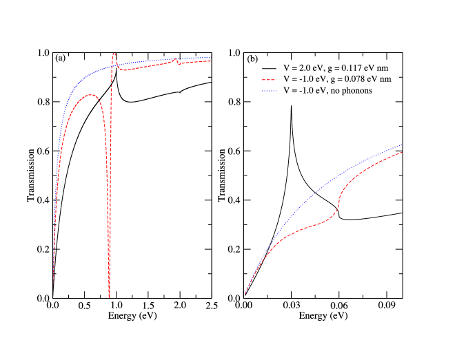
Figure 1: (a) Electron transmission probability through a delta potential. The solid black line represents a repulsive potential with an electron-phonon coupling constant $g=0.117$ eV nm. The dashed red line corresponds to transmission through an attractive delta potential with $g=0.078$ eV nm. In both cases, the electron is allowed to excite two local oscillator levels with energies $\hbar\omega$ = 1.0 eV and $2.0$ eV. The blue line is for $g=0$. (b) Electron transmission probability through a finite-width potential barrier/well of width $L=0.1$ nm. The solid black line represents a repulsive rectangular potential of strength $V_{0}=2.0$ eV with $g=0.117$ eV nm. The dashed red line corresponds to transmission through an attractive rectangular potential $V_{0}=-1.0$ eV with $g=0.078$ eV nm. The local oscillator levels are chosen to be at $\hbar\omega$= 0.03 eV and 0.06 eV, positioned at the centers of the rectangular potentials.

As a test of the validity of the propagation matrix method, we first examine two cases which have previously been studied in the literature. In Fig. 1(a), we show the transmission through repulsive (black) and attractive (red) delta potentials, which allow the excitation of two local vibrational modes at $\hbar\omega$ = 1.0 eV and 2.0 eV. For comparison, we also show the case (blue) without coupling to these local Einstein modes. In their absence, the transmission increases monotonically with the energy of the incoming electrons. However, in the presence of inelastic scattering channels resonance features in the form of spikes and dips in $T(E)$ occur at energies slightly below the local oscillator levels. They indicate the formation of bound statescai90 ; bagwell92 ; brandes02 , manifested by Fano features which for attractive potentials can completely suppress electron transmission right below the resonance energy (red line in Fig. 1(a)). These features arise from the strong feedback between inelastic and elastic scattering processes, and are easily missed in perturbative treatmentslevi89 . The parameters in Fig. 1 have been chosen identical to previously published data bagwell92 ; brandes02 to demonstrate full agreement of methods.

As shown in Fig. 1(b), the phenomenon of polaron-type bound state formation persists for finite-width wells and barriers. cai90 Here, the location of the Einstein scatterers are chosen at the center of the rectangular potential profiles. Bearing in mind experimentally relevant scales, we consider vibrational energies two orders of magnitude lower than in the Fig. 1(a), i.e. at $\hbar\omega=0.05$ eV and $0.10$ eV. In analogy to the case of delta potentials, resonances are observed at both energy levels. However, electron transmission is suppressed with respect to the case of delta potentials because of the finite spatial extent of the wells and barriers.

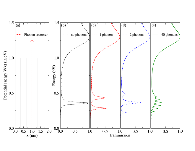
Figure 2: (a) Symmetric double rectangular potential with barrier width 0.4 nm, well width 0.6 nm, and barrier energy $V_{0}=$ 1.0 eV. A local phonon scatterer is located at the center of the double barrier. (b-e) Electron transmission probabilities for various numbers of accessible phonon channels. (b) corresponds to the case without electron-phonon interaction ($g=0$), (c) represents the transmission coefficient for one phonon channel, (d) for 2 phonon channels, and (e) for 40 phonon channels. In (c-e) the electron-phonon coupling is set to $g=0.04$ eV nm, and the phonon frequency is $\hbar\omega=0.01$ eV. With increasing number of phonon channels one observes the formation of a band.

Next, we turn to the case of electron transmission through more complex quantum well structures. Focusing on symmetric potential profiles, let us consider rectangular double barriers of length $0.4$ nm, separation $0.6$ nm, and height $V_{0}$ = 1 eV. A local Einstein scatterer is placed at the center of the well, as illustrated in Fig. 2(a). The vibrational energies are $\hbar\omega_{n}=n\hbar\omega$ with $\hbar\omega=0.01$ eV and $n=1,2,3,...$. In the absence of phonon scattering, shown in Fig. 2(b), one observes a bound state at $E=0.358$ eV which allows resonant tunneling with unit transmission. In the following, we examine the effects of inelastic scattering on this resonant feature. In the presence of a phonon scatterer with a single available inelastic channel at $\hbar\omega_{1}=0.01$ eV (Fig. 2(c)), the bound state is split into two satellites, separated by approximately equal energy gaps with respect to the energy of the original bound state. Such “side bands” have been the focus of numerous earlier studies. kim03 ; cai89 ; cai90 ; cai91 ; wu91 ; stovneng91 ; bagwell92 ; zhou93 ; bonca95 Note that for the semiconductor double barrier structures studied here the magnitudes of the energy splits between these phonon assisted satellite peaks are considerably larger than the weak coupling result, $E_{0}\pm\hbar\omega_{1}$, where $E_{0}$ is the energy of the resonance in the absence of inelastic scattering. This is due to strong renormalization of the bare electron-phonon coupling constant by the confinement of the electron wave function to the small well region, which will be discussed in more detail later on.

Here, we wish to examine how such phonon assisted satellite features merge into an impurity band with increasing number of available inelastic channels. The generalized propagation matrix method is particularly suited for this task, as the propagation matrix for the system only increases linearly with the number of added vibrational modes. The pattern which emerges from Fig. 2 is that the bound state splits into $n+1$ peaks, where $n$ is the number of phonon channels which are excited. For instance, in the case of one excited phonon with energy $0.01$ eV and electron-phonon coupling $\rm g=0.04eV\cdot nm$, we find the peaks to be at positions $E_{1}=0.2833$ eV and $E_{2}=0.4340$ eV (Fig. 2(c)), which differ from the zero-phonon case (Fig. 2(b)) by $\Delta_{1}=-0.0747$ eV and $\Delta_{2}=0.076$ eV. For two phonons (Fig. 2(d)), one finds 3 peaks at $E_{1}=0.2255$ eV, $E_{2}=0.3645$ eV, and $E_{3}=0.4875$ eV, giving shifts of $\Delta_{1}=-0.1325$ eV, $\Delta_{2}=0.0065$ eV and $\Delta_{3}=0.1295$ eV. This observation points to an interesting even-odd effect, whereby for odd numbers of phonon channels, there exists a central, non-bonding, peak, whereas for even numbers of phonon channels it is absent. It also implies that the satellites at $E_{n}\approx E_{0}\pm\hbar\omega_{n}$ are bonding/anti-bonding pairs. Before investigating this aspect of multi-phonon-assisted resonant tunneling more closely, let us point out that in the limit of many phonon channels (Fig. 2(e)) a low-energy band emerges. Note that the asymmetry in this impurity band is already anticipated in the asymmetry of the satellites for the few-phonon cases stovneng91 ; bagwell92 .

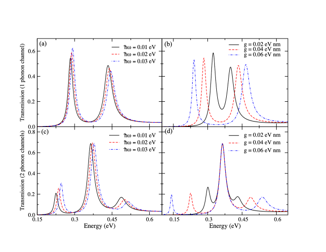
Figure 3: Electron transmission resonances for a double rectangular potential barrier with a phonon scatterer located at the center. The parameters are chosen identical to Fig. 2, unless otherwise specified. (a) and (b) correspond to a system with one phonon channel, and (c), (d) to a system with two phonon channels. In (a) and (c) the electron-phonon scattering strength is kept constant at $g$ = 0.04 eV nm, and the phonon energy $\hbar\omega$ is varied. One observes that the entire spectrum shifts to larger values of energy as $\hbar\omega$ increases. In (b) and (d) $\hbar\omega$ = 0.01 eV and $g$ is varied. In this case the gaps between the transmission resonance peaks widen with with increasing $g$. For two phonon channels, the central peak does not shift as $g$ is varied.

In Fig. 3 we examine the effects of the electron-phonon coupling and the vibrational energies on resonant transmission through the same double barrier potential shown in Fig. 2(a), i.e. we focus on the low-energy transmission peaks. The case of one available phonon channel is studied in Figs. 3(a) and (b), and the case of two phonon channels is illustrated in Figs. 3(c) and (d). Let us first keep the electron-phonon coupling constant at $\rm g=0.04eV\cdot nm$, and vary the energy of the vibrational levels. As observed in Figs. 3(a) and (c), increasing values of $\hbar\omega$ cause the entire spectrum of transmission resonances to shift to higher energies, whereas the gaps between the peaks remain constant. If instead we keep the vibrational energies fixed, i.e. at $\hbar\omega=0.01$ eV, and vary $g$, the gaps between peaks are found to increase as $g$ increases (see Table 1). Note that for the case of even numbers of phonon channels the central non-bonding peak does not shift with increasing $g$, whereas as the bonding/antibonding peaks move to higher and lower energies respectively.

Table 1: Gap between bonding and antibonding peaks for different values of electron-phonon coupling $g$

$\rm g(eV\cdot nm)$	0.02	0.04	0.06
$\Delta$ (1 phonon)	0.074 eV	0.147 eV	0.221 eV
$\Delta$ (2 phonons)	0.104 eV	0.209 eV	0.314 eV

The observation of bound state energy splitting when there are Einstein phonon channels in the system is analogous to degeneracy breaking in the linear Stark effect. For sufficiently small electron-phonon coupling, we can compute the first order energy shift quantitatively by treating the phonon energy and electron-phonon interaction terms in the Hamiltonian (1) as perturbations and by using time-independent degenerate perturbation theory to calculate the resulting energy shifts. The unperturbed eigenstates are denoted by $|x,n\rangle$, where $n$ is the phonon quantum number and $x$ denotes the electron position in the well region of the potential profile $x\in[0,L]$. In order to make analytical progress, the electron wave function is approximated by the infinite well wavefunction $\Psi(x)\approx\text{sin}(\pi x/L)/\sqrt{L}$, where $L$ is the length of the well. The resulting perturbation matrix has elements $\langle x,n|\sum_{x_{i}}\hbar\omega b^{\dagger}_{x_{i}}b_{x_{i}}+g\sum_{x_{i},k,k^{\prime}}\delta(x-x_{i})\left(b^{\dagger}_{x_{i}}+b_{x_{i}}\right)c^{\dagger}_{k}c_{k^{\prime}}|x,n\rangle$, which for the case of one phonon channel yields the $2\times 2$ perturbation matrix

$$\hat{P}=\left(\begin{array}[]{cc}0&g/L\\ g/L&\hbar\omega\\ \end{array}\right).$$ (5)

Assuming that the impurity site is located at $x_{0}=L/2$, we have $\text{sin}(\pi x_{0}/L)=1$. The energy shifts are calculated by diagonalization of the perturbation matrix and are given by

$$\lambda=\frac{\hbar\omega}{2}\pm\sqrt{\left(\frac{\hbar\omega}{2}\right)^{2}+\left(\frac{g}{L}\right)^{2}}.$$ (6)

In practice, the well width $L$ can be made rather small, even compared to the scale of molecular junctions. This can lead to a significant renormalization of the electron-phonon coupling constant, $g\rightarrow g/L$, which in turn explains the the relatively large energy gaps between the phonon assisted satellites, observed in the propagation matrix results.

To further illustrate how the bound state energies depend on the phonon energy and the electron-phonon coupling, we plot the lower and higher bound state energies as a function of $\hbar\omega$ (Figs. 4(a) and 4(c)), and as a function of $g$ (Figs. 4(b) and 4(d)).

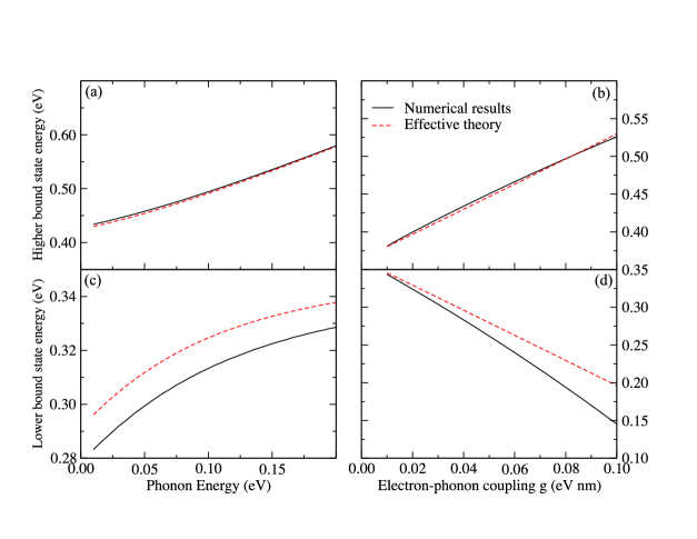
Figure 4: Bound state energies in a double rectangular potential barrier with one phonon scatterer at the center (as depicted in Fig. 2(a)). For the case of one phonon channel, the energies of the two resulting transmission resonance peaks are plotted as functions of the electron-phonon coupling constant $g$ and of the phonon energy $\hbar\omega$. Exact numerical results (solid black lines) are compared with the effective theory (dashed red lines) described in the text. In (a) and (c) the electron-phonon coupling is kept constant at $g=0.04$ eV nm, and in (b) and (d) the phonon energy is kept constant at $\hbar\omega=0.01$ eV. In (a) and (b), for the higher bound state energies, the effective theory reproduces remarkably well the numerical results. In (c), the effective theory and numerical results are off-set by approximately $0.02$ eV. In (d), the effective theory matches the numerical results for small values of $g$. For instance, when $g=0.04$ eV nm, the effective theory overestimates the lower bound state energy by $0.01$ eV.

The accuracy of the effective theory compared to the numerical results of the full propagation matrix calculation is striking, in particular for predicting the higher bound state energy (Figs. 4(a) and 4(b)). For the lower bound state, the accuracy increases for smaller $g$ (Fig. 4(d)), although for a fixed value of $\rm g=0.04eV\cdot nm$ and variable $\hbar\omega$ the effective theory predicts a lower bound state off-set by about $0.02$ eV with respect to the full propagation matrix calculation (Fig. 4(c)). This difference is of the order of the phonon energy and one order of magnitude lower than the bound state energy. However we notice that although the curves for the effective theory and numerical results are off, they present the same qualitative behavior. Therefore, one can affirm that the effective theory reproduces the numerical results with striking accuracy for small values of $g$. The same procedure can be repeated for any number of phonon channels with similar results.

Finally, let us turn to the current-voltage characteristics caused by phonon assisted transmission features. As shown in Fig. 5(a), application of an external electric field yields a spatial gradient in the potential energy profile. The resulting current flow is determined from the transmission functions $T(E,V)$ at given voltage biases $V$ via an integral

$$I(V)=\int_{0}^{V_{0}}T(E,V)dE,$$ (7)

where the energy window $[0,V_{0}]$ for currents through semiconductor heterostructures is small compared to molecular junctions. As a result of this, the $I(V)$ dependence shown in Fig. 5(c) inherits the peak structure of the individual transmission curves, some of which are shown in Fig. 5(b). This is an important difference from the step-like $I(V)$ curves reported in measurements of molecular junctions.mitra04 ; braig03

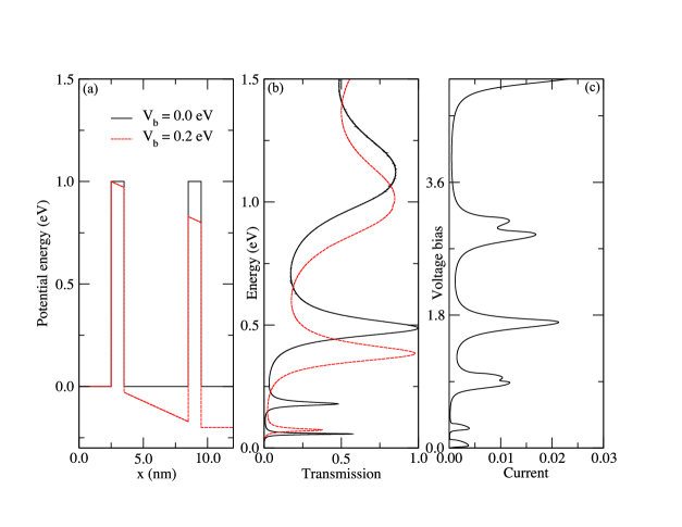
Figure 5: (a) Potential double barrier with thickness of 1.0 nm and separation of 5.0 nm. The height of the barrier is 1.0 eV, and the electronic effective mass is $0.07m_{e}$. (b) Transmission vs. energy curves for one excited phonon at the center of the potential well. In the presence of a voltage bias across the heterostructure, this curve is shifted towards lower energies. (c) Current-voltage curve for the double barrier in (a). The two small peaks at low voltage bias ($V_{b}$) correspond to the two low energy peaks in (b). The calculation of current is done by integrating the transmission over an energy window from 0 eV to 50 meV.

IV Conclusion

In summary, we have investigated how quantum well electron-phonon resonances are affected by the presence of several inelastic channels in the phonon spectrum. Using a generalized propagation matrix method for multiple eleastic and inelastic transmission channels, we determined the highly non-perturbative effects of scattering by Einstein phonons on the electron transmission through potential structures. In particular, we observed a characteristic splitting of the bound state resonances into satellite peaks. The presence or absence of a non-bonding resonance reflects the parity associated with even vs. odd numbers of accessible inelastic channels. Furthermore, in the limit of many available channels, the formation of low-energy impurity bands was observed. The dependence of the resonance satellites on the electron-phonon coupling strength and on the phonon energies could be reproduced using an effective model, which works well within the limits of perturbation theory. One promise of the multi-channel propagation matrix method which is developed here lies in the ability to study highly asymmetric quantum systems with strongly interacting itinerant and local features. A further direction to pursue is to depart from strictly local oscillators, which are nevertheless important for nanoelectronics, and to consider spatially extended phonon scattering regions.

V Acknowledgments

We wish to thank A.F.J. Levi and B. Normand for useful comments, and acknowledge support by the Department of Energy under grant DE-FG02-05ER46240.

VI Appendix

As an illustration of how to construct the generalized propagation matrix in practice, let us consider the example of a rectangular potential barrier given by

$$V(x)=\left\{\begin{array}[]{rl}0,&x<a\\ V_{0},&a\leq x\leq b\\ 0,&x>b\end{array}\right.$$ (11)

The wavefunctions are written as superpositions of plane waves,

$$\psi_{n}(x<a) = a_{n}e^{ik_{n}x}+b_{n}e^{-ik_{n}x},k_{n}=\sqrt{E-n\omega},$$ (12)

$$\psi_{n}(x>b) = t_{n}e^{ik_{n}x},k_{n}=\sqrt{E-n\omega},$$ (13)

$$\psi_{n}(a\leq x\leq b) = c_{n}e^{-\kappa_{n}x}+d_{n}e^{\kappa_{n}x},\kappa_{n}=\sqrt{V_{0}-E-n\omega},$$ (14)

where $n$ represents the available phonon channels. It is assumed as an initial condition that the incident electrons enter the potential structure from the left, i.e. $a_{0}=1,a_{n\neq 0}=0$.

To determine the transmission coefficients for the elastic ($t_{n=0}$) and inelastic ($t_{n\neq 0}$) channels we use the propagation matrix method, matching the conditions $\psi_{n,j}=\psi_{n,j+1}$ and $d\psi_{n,j}/dx=d\psi_{n,j+1}/dx$ at each boundary. In the absence of phonon scattering ($n=0$), the propagation matrix $\rho$ of the system is obtained by multiplication of the step matrices (at $x=a$ and $x=b$) and the free propagation matrix for $a\leq x\leq b$,

$$\hat{\rho}=\hat{\rho}_{step}^{a}\hat{\rho}_{free}^{L}\hat{\rho}_{step}^{b},$$ (15)

which are given by

$$\hat{\rho}_{step}^{a}=\frac{1}{2}\left(\begin{array}[]{cc}1+\frac{\kappa_{0}}{k_{0}}&1-\frac{\kappa_{0}}{k_{0}}\\ 1-\frac{\kappa_{0}}{k_{0}}&1+\frac{\kappa_{0}}{k_{0}}\end{array}\right)$$ (16)

$$\hat{\rho}_{step}^{b}=\frac{1}{2}\left(\begin{array}[]{cc}1+\frac{k_{0}}{\kappa_{0}}&1-\frac{k_{0}}{\kappa_{0}}\\ 1-\frac{k_{0}}{\kappa_{0}}&1+\frac{k_{0}}{\kappa_{0}}\end{array}\right)$$ (17)

And in the interval $a\leq x\leq b$:

$$\hat{\rho}_{free}^{L}=\left(\begin{array}[]{cc}e^{\kappa_{0}L}&0\\ 0&e^{-\kappa_{0}L}\\ \end{array}\right)$$ (18)

with $L=b-a$.

In order to find the transmission probability, we need to solve the matrix equation $\hat{\rho}\textbf{t}=\textbf{a}$ where the coefficients of the wave functions (7) and (8) are the elements of a and t, respectively:

$$\left(\begin{array}[]{cc}\rho_{11}&\rho_{12}\\ \rho_{21}&\rho_{22}\end{array}\right)\left(\begin{array}[]{c}t_{0}\\ 0\end{array}\right)=\left(\begin{array}[]{c}a_{0}\\ b_{0}\end{array}\right)$$ (19)

For this system without phonon channels, the transmission probability $T(E)$ is simply:

$$|t_{0}|^{2}=\left|\frac{a_{0}}{\rho_{11}}\right|^{2}$$ (20)

If instead phonon scatterer centers are present, we do not have the above condition on the derivative, but rather integrate Schrödinger’s equation around $x=0$ (from $-\epsilon$ to $+\epsilon$). If for instance, we add a phonon scatterer at $x=a$ in the same potential barrier, we have for the step and free matrices are:

$$\hat{\rho}_{step}^{a}=\frac{1}{2}\left(\begin{array}[]{cccc}1+\frac{i\kappa_{0}}{k_{0}}&1-\frac{i\kappa_{0}}{k_{0}}&\frac{igm}{k_{0}\hbar^{2}}&\frac{igm}{k_{0}\hbar^{2}}\\ 1-\frac{i\kappa_{0}}{k_{0}}&1+\frac{i\kappa_{0}}{k_{0}}&\frac{-igm}{k_{0}\hbar^{2}}&\frac{-igm}{k_{0}\hbar^{2}}\\ \frac{igm}{k_{1}\hbar^{2}}&\frac{igm}{k_{1}\hbar^{2}}&1+\frac{i\kappa_{1}}{k_{1}}&1-\frac{i\kappa_{1}}{k_{1}}\\ \frac{-igm}{k_{1}\hbar^{2}}&\frac{-igm}{k_{1}\hbar^{2}}&1-\frac{i\kappa_{1}}{k_{1}}&1+\frac{i\kappa_{1}}{k_{1}}\end{array}\right)$$ (21)

$$\hat{\rho}_{step}^{b}=\frac{1}{2}\left(\begin{array}[]{cccc}1+\frac{k_{0}}{\kappa_{0}}&1-\frac{k_{0}}{\kappa_{0}}&0&0\\ 1-\frac{k_{0}}{\kappa_{0}}&1+\frac{k_{0}}{\kappa_{0}}&0&0\\ 0&0&1+\frac{k_{1}}{\kappa_{1}}&1-\frac{k_{1}}{\kappa_{1}}\\ 0&0&1-\frac{k_{1}}{\kappa_{1}}&1+\frac{k_{1}}{\kappa_{1}}\end{array}\right)$$ (22)

$$\hat{\rho}_{free}^{L}=\left(\begin{array}[]{cccc}e^{\kappa_{0}L}&0&0&0\\ 0&e^{-\kappa_{0}L}&0&0\\ 0&0&e^{\kappa_{1}L}&0\\ 0&0&0&e^{-\kappa_{1}L}\end{array}\right)$$ (23)

Once again we determine $T(E)$ by solving $\hat{\rho}\textbf{t}=\textbf{a}$. However, now we have two transmission coefficients $t_{0}$ and $t_{1}$, one for each phonon channel, and the transmission probability is given by:

$$T(E)=|t_{0}|^{2}+\frac{k_{1}(E)}{k_{0}(E)}|t_{1}|^{2}.$$ (24)

References

- (1) V. J. Goldman, D. C. Tsui, and J. E. Cunningham, Phys. Rev. B 36, 7635 (1987).
- (2) G. S. Boebinger, A. F. J. Levi, S. Schmitt-Rink, A. Passner, L. N. Pfeiffer, and K. W. West, Phys. Rev. Lett. 65, 235 (1990).
- (3) J. G. Chen, C. H. Yang, M. J. Yang, and R. A. Wilson, Phys. Rev. B 43, 4531 (1991).
- (4) A. K. Geim, T. J. Foster, A. Nogaret, N. Mori, P. J. McDonnell, N. La Scala, Jr., P. C. Main, and L. Eaves, Phys. Rev. B 50, 8074 (1994).
- (5) G. Kim, D.W. Roh, and S.W. Paek, Appl. Phys. Lett. 83, 695 (2003).
- (6) A. Nitzan and M.A. Ratner, Science 300, 1384 (2003).
- (7) C. Benesch, M. Cizek, M. Thoss, and W. Domcke, Chem. Phys. Lett. 430, 355 (2006).
- (8) A. Mitra, I. Aleiner, and A. J. Millis, Phys. Rev. B 69, 245302 (2004).
- (9) S. Braig and K. Flensberg, Phys. Rev. B 68, 205324 (2003); K. Flensberg, Phys. Rev. B 68, 205323 (2003).
- (10) M. Galperin, M.A. Ratner and A. Nitzan, J. Phys.: Condens. Matter 19, 103201 (2007).
- (11) A. Yacoby, M. Heiblum, D. Mahalu, and H. Shtrikman, Phys. Rev. Lett. 74, 4047 (1995).
- (12) E. Buks, R. Schuster, M. Heiblum, D. Mahalu, V. Umansky, and H. Shtrikman, Phys. Rev. Lett. 77, 4664 (1996).
- (13) B. Y. Gelfand, S. Schmitt-Rink, and A. F. J. Levi, Phys. Rev. Lett. 62, 1683 (1989).
- (14) W. Cai, T. F. Zheng, P. Hu, B. Yudanin, and M. Lax, Phys. Rev. Lett. 63, 418 (1989).
- (15) W. Cai, P. Hu, T. F. Zheng, B. Yudanin, and M. Lax, Phys. Rev. B 41, 3513 (1990).
- (16) W. Cai, T. F. Zheng, P. Hu, and M. Lax, Mod. Phys. Lett. B 5, 173 (1991).
- (17) X. Wu and S. E. Ulloa, Phys. Rev. B 44, 13148 (1991).
- (18) J. A. Stovneng, E. H. Hauge, P. Lipavsky and V. Spicka, Phys. Rev. B. 44, 13595 (1991).
- (19) P.F. Bagwell and R.K. Lake, Phys. Rev. B 46, 15329 (1992).
- (20) C.H. Grein, E. Runge, and H. Ehrenreich, Phys. Rev. B 47, 12590 (1993).
- (21) N. Zhou, Q. Chen, and M. Willander, J. Appl. Phys. 75, 1829 (1993).
- (22) J. Bonca and S. A. Trugman, Phys. Rev. Lett. 75, 2566 (1995).
- (23) J. Bonca and S. A. Trugman, Phys. Rev. Lett. 79, 4874 (1997).
- (24) K. Haule and J. Bonca, Phys. Rev. B 59, 13087 (1999).
- (25) J. M. Mohaidat, K. Shum, and R. R. Alfano, Phys. Rev. B 48, 8809 (1993).
- (26) T. Brandes and J. Robinson, Phys. Stat. Sol. B, 234, 378 (2002).
- (27) A. F. J. Levi, “Applied Quantum Mechanics”, pp. 167-237, Cambridge University Press (2003).
- (28) See e.g. Zarea et al, Electronics Lett. 28, 264 (1992); Magno et al, J. Appl. Phys. 90 ,6177 (2001); Narihiro et al, Appl. Phys. Lett. 70, 105 (1997); Mendez et al, Phys. Rev. B 43, 5196 (1991); Chow et al, Appl. Phys. Lett. 61, 1685 (1992).