Impact of modulation on CMB $\mn@boldsymbol{B}$-mode polarization experiments

Abstract

We investigate the impact of both slow and fast polarization modulation strategies on the science return of upcoming ground-based experiments aimed at measuring the $B$-mode polarization of the cosmic microwave background. Using detailed simulations of the C_ℓOVER  experiment, we compare the ability of modulated and un-modulated observations to recover the signature of gravitational waves in the polarized CMB sky in the presence of a number of anticipated systematic effects. The general expectations that fast modulation is helpful in mitigating low-frequency detector noise, and that the additional redundancy in the projection of the instrument’s polarization sensitivity directions onto the sky when modulating reduces the impact of instrumental polarization, particularly for fast modulation, are borne out by our simulations. Neither low-frequency polarized atmospheric fluctuations nor systematic errors in the polarization sensitivity directions are mitigated by modulation. Additionally, we find no significant reduction in the effect of pointing errors by modulation. For a C_ℓOVER-like experiment, pointing jitter should be negligible but any systematic mis-calibration of the polarization coordinate reference system results in significant $E$-$B$ mixing on all angular scales and will require careful control. We also stress the importance of combining data from multiple detectors in order to remove the effects of common-mode systematics (such as un-polarized $1/f$ atmospheric noise) on the measured polarization signal. Finally we compare the performance of our simulated experiment with the predicted performance from a Fisher analysis. We find good agreement between the (optimal) Fisher predictions and the simulated experiment except for the very largest scales where the power spectrum estimator we have used introduces additional variance to the $B$-mode signal recovered from our simulations. In terms of detecting the total $B$-mode signal, including lensing, the Fisher analysis and the simulations are in excellent agreement. For a detection of the primordial $B$-mode signal only, using an input tensor-to-scalar ratio of $r=0.026$, the Fisher analysis predictions are $\sim 20$ per cent. better than the simulated performance.

1 Introduction

There is currently a great deal of interest in the rapidly evolving field of observations of the polarization of the cosmic microwave background (CMB). This interest stems from the fact that such observations have the potential to discriminate between inflation and other early-universe models through their ability to constrain an odd-parity $B$-mode polarization component induced by a stochastic background of gravitational waves at the time of last scattering (Kamionkowsky, Kosowksy & Stebbins, 1997; Seljak & Zaldarriaga, 1997).

From an observational point of view, we are still a long way off from a detection of this $B$-mode signature of inflation. However, much progress has been made recently with the detection of the much stronger $E$-mode polarization signal on large scales by the WMAP  experiment (Page et al., 2007; Nolta et al., 2008). On smaller scales, a growing number of balloon-borne and ground-based experiments have also measured $E$-mode polarization including DASI  (Leitch et al., 2005), CBI  (Sievers et al., 2007), BOOMERANG  (Montroy et al., 2006), MAXIPOL  (Wu et al., 2007), CAPMAP  (Bischoff et al., 2008) and QUaD  (Pryke et al., 2009). Most recently, the high precision measurement of small-scale polarization by the QUaD  experiment has, for the first time, revealed a characteristic series of acoustic peaks in the $E$-mode spectrum and put the strongest upper limits to date on the small-scale $B$-mode polarization signal expected from gravitational lensing by large-scale structure.

Building on the experience gained from these pioneering experiments, a new generation of experiments is now under construction with the ambitious goal of observing the primordial $B$-mode signal. Observing this signal is one of the most challenging goals of modern observational cosmology. There are a number of reasons why these types of observations are so difficult. First and foremost, the sought-after signal is expected to be extremely small – in terms of the tensor-to-scalar ratio, the RMS polarization signal from primordial $B$-modes is $0.4\sqrt{r}\,\mu\mathrm{K}$, and the current 95 per cent limit $r<0.22$ from WMAP  temperature and $E$-mode polarization plus distance indicators (Komatsu et al., 2009) implies an RMS $<180\,\mathrm{nK}$. Secondly, polarized emission from our own galaxy and from extra-Galactic objects act as a foreground contaminant in observing the CMB polarized sky. Although our knowledge of such polarized foregrounds is currently limited, particularly at the higher frequencies $\mathrel{\hbox to0.0pt{\lower 4.0pt\hbox{\hskip 1.0pt$\sim$}\hss}\raise 1.0pt\hbox{$>$}}100\,\mathrm{GHz}$ of relevance to bolometer experiments, models suggest that such contamination could be an order of magnitude larger than the sought-after signal on the largest scales (e.g. Amblard, Cooray & Kaplinghat 2007). Thirdly, gravitational lensing by large-scale structure converts $E$-modes into $B$-modes on small to medium scales (see Lewis & Challinor 2006 for a review) and acts as a source of confusion in attempts to measure the primordial $B$-mode signal (Knox & Song, 2002; Kesden, Cooray & Kamionkowski, 2002). Note however that the lensing $B$-mode signal is a valuable source of cosmological information in its own right and can be used to put unique constraints on dark energy and massive neutrinos (e.g. Kaplinghat, Knox & Song 2003; Smith, Challinor & Rocha 2006). Unfortunately these latter two effects (foreground contamination and weak gravitational lensing) contrive in such a way as to render $B$-mode polarization observations subject to contamination on all angular scales (the primordial $B$-mode signal is dominated by foregrounds on large scales whilst on smaller scales it is swamped by the lensing signal). Last, but not least, exquisite control of systematic and instrumental effects will be required, to much better than $100\,\mathrm{nK}$, before any detection of $B$-modes can be claimed. The sought-after signal is so small that systematic and instrumental effects considered negligible for an exquisitely precise measurement of $E$-modes say, could potentially ruin a detection of $B$-modes, if left uncorrected. One possible approach to mitigating some of these systematics in hardware is to modulate the incoming polarization signal such that it is shifted to higher frequency and thus away from low-frequency systematics which would otherwise contaminate it. There are a number of techniques for achieving this including the use of a rotating half-wave plate (HWP; e.g. Johnson et al. 2007), phase-switching, or Faraday rotation modulators (Keating et al., 2003).

In this paper, we investigate the ability of modulation techniques that are either slow or fast with respect to the temporal variation of the signal to mitigate a range of possible systematic effects. Our analysis is based on simulations, and the subsequent analysis, of data from a ground-based CMB $B$-mode polarization experiment. Previous investigations of the impact of systematic effects on $B$-mode observations include the analytic works of Hu, Hedman & Zaldariagga (2003), O’Dea, Challinor & Johnson (2007) and Shimon et al. (2008), as well as the simulation-based analysis of MacTavish et al. (2008) who based their study on signal-only simulations of the SPIDER  experiment. The simulation work presented here is complementary to these previous analyses but we also take our analysis further by including realistic noise in our simulations — we are thus able to quantify not only any bias found, but also any degradation of performance due to the presence of systematic effects. Our work makes use of a detailed simulation pipeline which we have created in the context of the C_ℓOVER  experiment. Although the precise details of our simulations are specific to C_ℓOVER , our general conclusions regarding the impact of modulation on a variety of systematic effects are relevant to all upcoming ground-based $B$-mode experiments and many of them are also relevant for both balloon-borne and space-based missions.

The paper is organised as follows. In Section 2, we review the relevant upcoming $B$-mode polarization experiments. Section 3 describes our simulation technique and the systematic effects we have considered. In Section 4, we describe the map-making and power spectrum estimation techniques that we use to analyse the simulated data. Section 5 presents the results from our main analysis of systematic effects. We discuss our results in Section 6 where, for clarity, we group the possible systematic effects considered into those that are, and those that are not, mitigated by a modulation scheme. In this section, we also demonstrate the importance of combining information from multiple detectors during analysis and compare the simulated performance of C_ℓOVER  to the predicted performance from a Fisher analysis. Our conclusions are summarised in Section 7. Finally, Appendix A develops a simple model of the spurious $B$-mode power produced by pointing jitter for experiments with a highly redundant scan strategy.

2 CMB polarization experiments

A host of experiments are currently under construction (one is, in fact, already observing) with their primary goal being to constrain the tensor-to-scalar ratio, and thus the energy scale of inflation, through observations of the $B$-mode component of the CMB. Here, we give a short summary of the planned experiments.

(i) Ground-based experiments:

• BICEP/BICEP-2/KECK array: The BICEP  experiment (Yoon et al., 2006) has recently completed its third and final season of operation from the South Pole. The experiment consisted of a total of 98 polarization-sensitive bolometers (PSBs) at 100 and 150 GHz. The optical design is very clean but with the downside of poor resolution – 45 arcmin full-width at half-maximum (FWHM) at 150 GHz – which limits the target multipole range to $\ell<300$. The stated target sensitivity is $r=0.1$. In the first observing season, three 100 GHz pixels and three 150 GHz pixels were equipped with Faraday rotation modulators and two pixels operated at 220 GHz. BICEP-2 will consist of an upgrade to the BICEP  telescope with a 150 GHz 512-element array of antenna-coupled detectors. It will be deployed to the South Pole in November, 2009. The KECK array will consist of three BICEP-2-like telescopes (at 100, 150 and 220 GHz). It is hoped to be installed on the DASI  mount (previously occupied by QUaD) in November 2010. The nominal goal of this array is $r=0.01$.

• C_ℓOVER: For an up-to-date overview see North et al. (2008). C_ℓOVER  is a three-frequency (97, 150 and 225 GHz) instrument to be sited at Pampa La Bola in the Atacama desert in Chile. It will have 576 single-polarization transition-edge sensors (TES), split equally among the three frequencies. The beam size of $\sim$ 5.5 arcmin FWHM at 150 GHz will sample the multipole range $25<\ell<2000$. The target sensitivity is $r\sim 0.03$ and the polarization signal will be modulated with a HWP. The 97 GHz instrument is expected to be deployed to Chile in late 2009 with the combined 150/225 GHz instrument to follow soon after in 2010.

• QUIET: See Samtleben (2008) for a recent overview. QUIET  is unique among planned $B$-mode experiments in that it uses pseudo-correlation HEMT-based receivers rather than bolometers. It will observe from Chile using the CBI mount – a planned second phase will involve upgrading to $\sim 1000$ element arrays and relocation of the 7-m Crawford Hill antenna from New Jersey to Chile. QUIET  will observe at 40 and 90 GHz. The target sensitivity for the second phase is $r\sim 0.01$.

• POLARBEAR: A three-frequency (90, 150 and 220 GHz) single-dish instrument to be sited in the Inyo Mountains, CA for its first year of operation, after which it will be relocated to the Atacama desert in Chile. It will use 1280 TES bolometers at each frequency with polarization modulation from a HWP. The planned beam size is 4 arcmin (FWHM) at 150 GHz. The target sensitivity is $r=0.015$ for the full instrument.

• BRAIN: See Charlassier (2008) for a recent review. BRAIN  is a unique bolometric interferometer project (c.f. DASI, CBI) to be sited on the Dome-C site in Antarctica. The final instrument will have $\sim 1000$ bolometers observing at 90, 150 and 220 GHz. BRAIN  will be primarily sensitive to multipoles $50<\ell<200$. The full experiment is planned to be operational in 2011 and the stated target sensitivity is $r=0.01$.

(ii) Balloon-borne experiments

• EBEX: See Oxley et al. (2004) for a summary. EBEX  will observe at 150, 250 and 410 GHz and will fly a total of $1406$ TES with HWP modulation. The angular resolution is 8 arcmin and the target multipole range is $20<\ell<2000$. The stated target sensitivity is $r=0.02$. A test flight is planned for 2009 and a long-duration balloon (LDB) flight is expected soon after.

• SPIDER: See Crill et al. (2008) for a recent description. SPIDER  will deploy $\sim 3000$ antenna-coupled TES observing at 96, 145, 225 and 275 GHz, with a beam size of $\sim 40$ arcmin at 145 GHz. The target multipole range is $10<\ell<300$. A 2-6 day first flight is planned for 2010. The target sensitivity is $r=0.01$. Signal modulation will be provided by a (slow) stepped HWP and fast gondola rotation.

• PIPER: This balloon experiment will deploy a focal plane of 5120 TES bolometers in a backshort-under-grid (BUG) configuration. Each flight of PIPER  will observe at a different frequency, covering 200, 270, 350 and 600 GHz after the four planned flights. The beam size is $\sim 15$ arcmin, corresponding to a target multipole range $\ell<800$. The first element of the optical system is a variable polarization modulator (VPM). The entire optical chain, including the modulators, are cooled to 1.5 K so that PIPER  observes at the background limit for balloon altitudes. Including removal of foregrounds, the experiment has the sensitivity to make a $2\sigma$ detection of $r=0.007$. The first flight is scheduled for 2013.

(iii) Space missions

• PLANCK: See the publication of the Planck Collaboration (2006) for a detailed review of the science programme. PLANCK  will measure the temperature in nine frequency bands, seven of which will have (some) polarization sensitivity. The polarized channels (100, 143, 217 and 353 GHz) of the high-frequency instrument (HFI) use similar PSBs to those deployed on BOOMERANG  and have beam sizes 5–9.5 arcmin. For low $r$, sensitivity to primordial gravitational waves will mostly come from the large-angle reionisation signature (Zaldarriaga, 1997) and $r=0.05$ may be possible if foregrounds allow. PLANCK  will be sensitive to the multipole range $2<\ell<3000$ and is scheduled to launch in 2009. The HFI has no active or fast signal modulation (i.e. other than scanning).

• CMBPOL/BPOL: Design studies have been conducted for satellite mission(s) dedicated to measuring primordial $B$-modes comprising $\sim 2000$ detectors with the ability to measure $0.001<r<0.01$ if foregrounds allow it (Bock et al., 2008; de Bernardis et al., 2008). The timescale for launch of any selected mission is likely beyond 2020.

3 Simulations

The C_ℓOVER  experiment will consist of two telescopes – a low frequency instrument with a focal plane consisting of 192 single-polarization 97 GHz TES detectors, and a high frequency instrument with a combined focal plane of 150 and 225 GHz detectors (192 of each). Note that we have not included foreground contamination in our simulations, so for this analysis, we consider only the 150 GHz detector complement – the corresponding reduction in sensitivity will approximate the effect of using the multi-frequency observations to remove foregrounds. Figure 1 shows the arrangement of the 150 and 225 GHz detectors on the high frequency focal plane. The detectors are arranged in detector blocks consisting of eight pixels each. Each pixel consists of two TES detectors which are sensitive to orthogonal linear polarizations. The polarization sensitivity of the eight detector pairs within a block are along, and at right angles to, the major axis of their parent block. The detector complement, both at 150 and 225 GHz, therefore consists of three ‘flavours’ of pixels with different polarization sensitivity directions. The 97 GHz focal plane (not shown) has a similar mix of detector orientations.

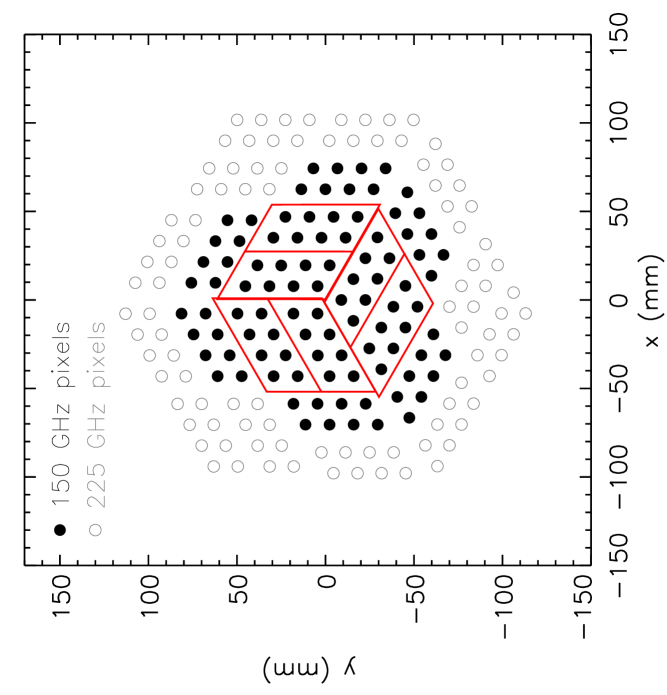
Figure 1: Layout of detectors on the C_ℓOVER  high frequency focal plane. Each point indicates a pixel comprising two TES detectors sensitive to orthogonal linear polarizations. The polarization sensitivity directions of detectors within each block are along, and at right angles to, the major axis of the block. The outlined 150 GHz detector blocks at the centre of the array are used in the simulations described here. The field of view of the entire array is $\sim 5\,{\rm deg}^{2}$.

3.1 Simulation parameters

Because simulating the full C_ℓOVER  experiment is computationally demanding (a single simulation of a two-year campaign at the full C_ℓOVER  data rate would require $\sim 10^{4}$ CPU-hours), we have scaled some of the simulation parameters in order to make our analysis feasible.

1. We simulate only half the 150 GHz detector complement and have scaled the noise accordingly. We have verified with a restricted number of simulations using all the 150 GHz detectors that the marginally more even coverage obtained across our field using all detectors has little or no impact on our results or conclusions. The 150 GHz detector blocks used in our simulations are indicated in Fig. 1 and include all three possible orientations of pixels on the focal plane.

2. The C_ℓOVER  detectors will have response times of $\sim 200\,\mu$s and so the data will be sampled at $\sim 1$ kHz in order to sample the detector response function adequately. Simulating at this rate is prohibitive so we simulate at a reduced data rate of $100$ Hz. For the C_ℓOVER  beam size (FWHM = 5.5 arcmin at 150 GHz) and our chosen scan speed ($0.25^{\circ}$/s), this data rate is still fast enough to sample the sky signal adequately.

3. C_ℓOVER  will observe four widely separated fields on the sky, each covering an area of $\sim 300\,{\rm deg}^{2}$, over the course of two years. Two of the fields are in the southern sky and two lie along the equator. For our analysis, we observe each of the four fields for a single night only and, again, we have scaled the noise levels to those appropriate for the full two-year observing campaign.

3.2 Observing strategy

Although optimisation of the observing strategy is not the focus of this work, a number of possible strategies have been investigated by the C_ℓOVER  team. For our analysis, we use the most favoured scan strategy at the time of writing. To minimise rapid variations in atmospheric noise, the two telescopes will scan back and forth in azimuth at constant elevation, allowing the field to rise through the chosen observing elevation. Every few hours, the elevation angle of the telescopes will be re-pointed to allow for field-tracking. Although the precise details of the scan are likely to change, the general characteristics of the scan and resulting field coverage properties will remain approximately the same due to the limitations imposed by constant-elevation scanning and observing from Atacama. The C_ℓOVER  telescopes are designed with the capability of scanning at up to $10^{\circ}$/s. However, for our analysis where we have considered C_ℓOVER  operating with a rotating HWP (Section 3.7), we have chosen a relatively slow scan speed of $0.25^{\circ}$/s in light of the HWP rotation frequency which we have employed ($f_{\lambda}=3$ Hz). Although the mode of operation of a HWP on C_ℓOVER  is still under development, a continuously rotating HWP is likely to be restricted to rotation frequencies of $f_{\lambda}<5$ Hz due to mechanical constraints (with current cryogenic rotation technologies, fast rotation, $\mathrel{\hbox to0.0pt{\lower 4.0pt\hbox{\hskip 1.0pt$\sim$}\hss}\raise 1.0pt\hbox{$>$}}5$ Hz, could possibly result in excessive heat generation). Figure 2 shows the coverage maps for a single day’s observing on one of the southern fields and on one of the equatorial fields. The corresponding maps for the other two fields are broadly similar. Note that, in the real experiment, we expect that somewhat more uniform field coverage than that shown in Fig. 2 will be achievable by employing slightly different scan patterns on different days.

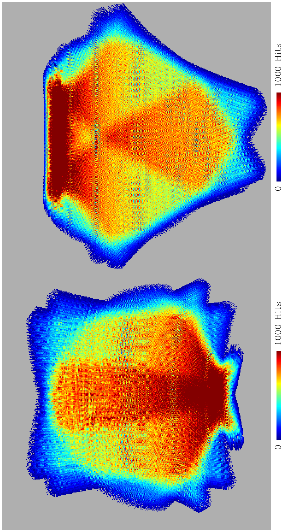
Figure 2: Hit-maps for one of the southern fields (left; RA 09:30 hrs , Dec -40.00^∘) and one of the equatorial fields (right; RA 04:00 hrs, Dec 0.00^∘) for a single day’s observation with half the 150 GHz detector complement. The central part of the fields (shown in yellow and red) are roughly $20^{\circ}$ in diameter. These maps have been constructed using a HEALPIX  resolution of $N_{\rm side}=1024$ corresponding to a pixel size $\sim$3.4 arcmin.

3.3 Signal simulations

We generate model $TT$, $EE$, $TE$ and $BB$ CMB power spectra using CAMB  (Lewis, Challinor & Lasenby, 2000). The input cosmology used consists of the best-fit standard $\Lambda$CDM model to the 5-year WMAP  data set (Hinshaw et al., 2009), but with a tensor-to-scalar ratio of $r=0.026$, chosen to match the C_ℓOVER  ‘target’ value. Realisations of CMB skies from these power spectra are then created using a modified version of the HEALPIX software (Górski et al., 2005). Our simulations include weak gravitational lensing but ignore its non-Gaussian aspects. Using only Gaussian simulations means that we slightly mis-estimate the covariance matrices of our power spectrum estimates, particularly the $B$-mode covariances (Smith, Hu & Kaplinghat, 2004; Smith, Challinor & Rocha, 2006). For the C_ℓOVER  noise levels, this is expected to have a negligible impact on the significance level of the total $B$-mode signal.

As part of the simulation process, the input CMB signal is convolved with a perfect Gaussian beam with FWHM $=5.5$ arcmin. Note that an important class of systematic effects which we do not consider in this paper are those caused by imperfect optics; see the discussion in Section 3.6.

For our analysis of the simulated data sets (Section 4) we have chosen to reconstruct maps of the Stokes parameters with a map resolution of $3.4$ arcmin (HEALPIX  $N_{\rm side}=1024$). Note that this pixel size does not fully sample the beam and it is likely that we will adopt $N_{\rm side}=2048$ for the analysis of real data. In order to isolate the effects of the various systematics we have considered, our simulated CMB skies have therefore been created at this same resolution — we can then be sure that any bias found in the recovered CMB signals is due to the systematic effect under consideration rather than due to a poor choice of map resolution. Note that our adopted procedure of simulating and map-making at identical resolutions, although useful for the specific aims of this paper, is not a true representation of a CMB observation. For real observations, pixelisation of the CMB maps will introduce a bias to the measured signal on scales comparable to the pixel size adopted.

Using the pointing registers as provided by the scan strategy and after applying the appropriate focal plane offsets for each detector, we create simulated time-streams according to

$$d_{i}=\left[T(\theta)+Q(\theta)\cos(2\phi_{i})+U(\theta)\sin(2\phi_{i})\right]/2,$$ (1)

where $\theta$ denotes the pointing and $T,Q$ and $U$ are the sky signals as interpolated from the input CMB sky map. The polarization angle, $\phi_{i}$ is, in general, a combination of the polarization sensitivity direction of each detector, any rotation of the telescope around its boresight, the direction of travel of the telescope in RA–Dec space and the orientation of the half-wave plate, if present.

3.4 Noise simulations

The C_ℓOVER  data will be subject to several different noise sources. Firstly, photon loading from the telescope, the atmosphere and the CMB itself will subject the data to uncorrelated random Gaussian noise. Secondly, the TES detectors used in C_ℓOVER  are subject to their own sources of noise which will possibly include low-frequency $1/f$ behaviour and correlations between detectors. Thirdly, the atmosphere also has a very strong $1/f$ component which will be heavily correlated across the detector array. Fortunately, the $1/f$ component of the atmosphere is known to be almost completely un-polarized and so can be removed from the polarization analysis by combining data from multiple detectors (see Section 6.2).

The white-noise levels due to loading from the instrument, atmosphere and CMB have been carefully modelled for the case of C_ℓOVER  observations from Atacama. We will not present the details here, but for realistic observing conditions and scanning elevations, we have calculated the expected noise-equivalent temperature (NET) due to photon noise alone to be $\approx 146\,\mu{\rm K}\sqrt{\rm s}$. We add this white noise component to our simulated signal time-streams for each detector as

$$d_{i}\rightarrow d_{i}+\frac{\rm NET}{2}\sqrt{f_{\rm samp}}g_{i},$$ (2)

where $f_{\rm samp}$ is the sampling frequency and $g_{i}$ is a Gaussian random number with $\mu=0$ and $\sigma=1$. Note that the white-noise level in the detector time streams is ${\rm NET}/2$ since the C_ℓOVER  detectors are half-power detectors (equation 1).

Using instrument parameters appropriate for the C_ℓOVER  detectors, we use the small-signal TES model of Irwin & Hilton (2005) to create a model noise power spectrum for the detector noise. This model includes both a contribution from the super-conducting SQUIDs which will be used to record the detector signals (e.g. Reintsema et al. 2003) and a contribution from aliasing in the Multi Channel Electronics (MCE; Battistelli et al. 2008) which will be used to read out the signals. For the instrument parameters we have chosen, the effective NET of the detector noise in our simulations is approximately equal to the total combined photon noise contribution from the atmosphere, the instrument and the CMB. Note however that for the final instrument, it is hoped that the detector NET can be reduced to half that of the total photon noise, thus making C_ℓOVER  limited by irreducible photon loading. The Irwin & Hilton (2005) small-signal TES model does not include a $1/f$ component to the detector noise so in order to investigate the impact of modulation on possible low-frequency detector noise, we add a heuristically chosen $1/f$ component to the detector noise model with knee frequencies in the range, $0.01<f_{\rm knee}<0.1$ Hz. The MCE system which will be used to read out the C_ℓOVER  data should have low cross-talk between different channels. However, correlations will be present at some level and so we include 10 per cent correlations between all of our simulated detector noise time-streams. Generally, to simulate stationary noise that is correlated in time and across the $N_{\rm det}$ detectors we proceed as follows. Let the noise cross-power spectrum between detector $d$ and $d^{\prime}$ be $P_{d,d^{\prime}}(f)$. Taking the Cholesky decomposition of this matrix at each frequency, $L_{d,d^{\prime}}(f)$, defined by

$$P_{d,d^{\prime}}(f)=\sum_{d^{\prime\prime}}L_{d,d^{\prime\prime}}(f)L_{d^{\prime},d^{\prime\prime}}(f),$$ (3)

we apply $L$ to $N_{\rm det}$ independent, white-noise time streams $g_{d}(f)$ in Fourier space,

$$g_{d}(f)\rightarrow\sum_{d^{\prime}}L_{d,d^{\prime}}(f)g_{d^{\prime}}(f).$$ (4)

The resulting time-streams, transformed to real space then possess the desired correlations between detectors. Here, we assume that the correlations are independent of frequency so that the noise cross-power spectrum takes the form

$$P_{d,d^{\prime}}(f)=C_{d,d^{\prime}}P(f),$$ (5)

where the correlation matrix $C_{d,d^{\prime}}=1$ for $d=d^{\prime}$ and $C_{d,d^{\prime}}=0.1$ otherwise. In practice, we use discrete Fourier transforms to synthesise noise with periodic boundary conditions (and hence circulant time-time correlations).

We use the same technique to simulate the correlated $1/f$ component of the atmosphere. We have measured the noise properties of the atmosphere from data from the QUaD  experiment (Hinderks et al., 2009). The 150 GHz frequency channel of QUaD  is obviously well matched to the C_ℓOVER  150 GHz channel although QUaD  observed the CMB from the South Pole rather than from Atacama. Although there are significant differences between the properties of the atmosphere at the South Pole and at Atacama (e.g. Bussmann, Holzapfel & Kuo 2005), the QUaD  observations still represent the best estimate of the $1/f$ noise properties of the atmosphere available at present. A rough fit of the QUaD  data to the model,

$$P(f)={\rm NET^{2}}\left[1+\left(\frac{f_{\rm knee}}{f}\right)^{\alpha}\right],$$ (6)

yields a knee frequency, $f_{\rm knee}=0.45$ Hz and spectral index, $\alpha=2.5$. Using this model power spectrum we simulated $1/f$ atmospheric noise correlated across the array in exactly the same way as was used for the detector noise. Fortunately, the $1/f$ component in the atmosphere is almost completely un-polarized. If there were no instrumental polarization, detectors within the same pixel (which always look in the same direction) would therefore be completely correlated with one another and detectors from different pixels would also be heavily correlated. For the correlated atmosphere, we therefore use a correlation matrix given by $C_{d,d^{\prime}}=1.0$ for $|d-d^{\prime}|\leq 1$ (i.e. for detector pairs) and $C_{d,d^{\prime}}=0.5$ otherwise. In the following sections, as one of the systematics we have investigated, we relax the assumption that the atmosphere is un-polarized.

Figure 3 compares the photon, atmospheric $1/f$ and detector noise contributions to our simulated data in frequency space. At low frequencies, the noise is completely dominated by the atmospheric $1/f$ while the white-noise contributions from photon loading (including the uncorrelated component of the atmosphere) and detector noise are approximately equal. Note that for observations without active modulation, and for the scan speed and observing elevations which we have adopted, the “science band” for the multipole range $20<\ell<2000$ corresponds roughly to $0.01<f<1$ Hz in time-stream frequency. In contrast, for our simulations which include a continuously rotating HWP, the temperature signal remains within the $0.01<f<1$ Hz frequency range but the polarized sky signal is moved to a narrow band centred on $\sim$12 Hz, well away from both the detector and atmospheric $1/f$ noise components (see Section 3.7 and Fig. 5). Note also that although the atmospheric $1/f$ dominates the detector $1/f$ at low frequency, the atmosphere is heavily correlated across detectors and can therefore be removed by combining detectors (e.g. differencing detectors within a pixel) but this is not true for the detector noise which is only weakly correlated between detectors. We demonstrate this in Fig. 4 where we plot a five-minute sample of simulated atmospheric and detector noise for the two constituent detectors within a pixel. Including the atmospheric $1/f$ component, the effective total NET per detector measured from our simulated time-streams is $293\,\mu{\rm K}\sqrt{\rm sec}$ whilst excluding atmospheric $1/f$, we measure $210\,\mu{\rm K}\sqrt{\rm s}$.

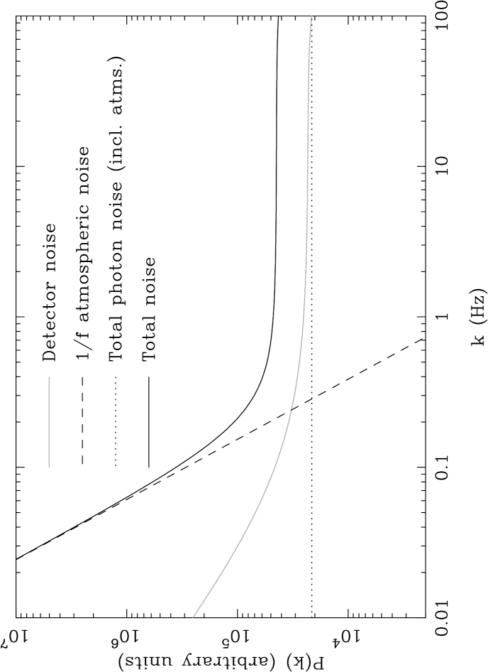
Figure 3: Frequency space comparison between the different noise sources in the simulations. The grey line shows the detector noise power spectrum (here with a $1/f$ component with knee frequency, $f_{\rm knee}=0.1$ Hz). The correlated component to the atmosphere is shown as the dashed line and the total photon noise (including atmospheric loading) is shown as the dotted line. For the simulation parameters we have adopted, the temperature sky-signal from multipoles $20<\ell<2000$ appears in the time-stream in the frequency range $0.01<f<1$ Hz. In the absence of fast modulation, the polarized sky signal also appears in this frequency range whereas in our simulations including fast modulation, the polarized sky signal appears in a narrow band centred on 12 Hz.

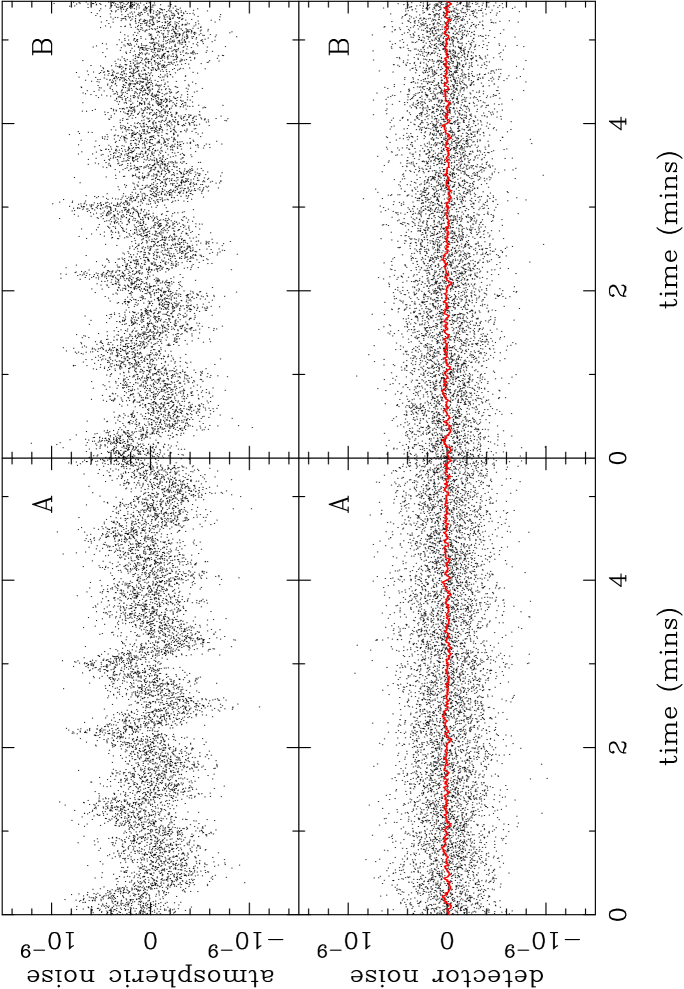
Figure 4: A five-minute sample of simulated noise time-stream for the two detectors within a pixel (denoted “A” and “B”) for both the atmospheric noise simulations (top) and for the detector noise simulations (bottom). The $1/f$ component in the atmospheric noise time-streams is 100 per cent correlated between the A and B detectors and can be removed entirely by differencing. In contrast the $1/f$ component in the detector noise (which is much weaker and not noticeable on this plot) is only weakly correlated between A and B and is not removed by differencing. For comparison, the signal-only time-streams are also plotted in the lower panels as the red curves.

3.5 Detector response

The Irwin & Hilton (2005) TES small-signal model mentioned above also provides us with an estimate of the detector response (the conversion from incident power to resultant current in the detectors). In this model, the power-to-current responsivity, $s_{I}(\omega)$, is given by

$$s_{I}(\omega)\propto\frac{1-\tau_{+}/\tau_{I}}{1+i\omega\tau_{+}}\frac{1-\tau_{-}/\tau_{I}}{1+i\omega\tau_{-}},$$ (7)

where $\omega=2\pi f$ is the angular frequency and $\tau_{+}$ and $\tau_{-}$ are the “rise time” and “fall time” (relaxation to steady state) after a delta-function temperature impulse. Here, $\tau_{I}$ is the current-biased thermal time constant. The impulse-response in the time domain is

$$s_{I}(t)\propto\frac{e^{-t/\tau_{+}}-e^{-t/\tau_{-}}}{\tau_{+}-\tau_{-}}\Theta(t),$$ (8)

where $\Theta(t)$ is the Heaviside step function. Note that the constant of proportionality in equation (7) (which is also predicted by the model) is essentially the calibration (gain) of the detectors. The simulated time-streams of equation (1) are converted to detector time-streams through convolution with this response function. Note that the photon noise and correlated atmospheric noise are added to the time-stream before convolution (and so are also convolved with the response function) while the detector noise is added directly to the convolved time-streams. The C_ℓOVER  detectors are designed to be extremely fast with time-constants $\tau_{\pm}<1\,{\rm ms}$. For our simulations, we have used time-constants predicted by the small-signal TES model for C_ℓOVER  instrument parameters of $\tau_{+}=300\,\mu{\rm s}$ and $\tau_{-}=322\,\mu{\rm s}$.

Note that for our chosen scan speed of $0.25^{\circ}$/s, the effect of the response function on the signal component in the simulations is small in the absence of fast modulation – the C_ℓOVER  detectors are so fast that signal attenuation and phase differences introduced by convolution with the detector response only become important at high frequencies, beyond the frequency range of the sky signals. For our simulations without fast modulation, sky signals from multipoles $\ell\sim 2000$ will appear in the time-stream at $\sim$ 1 Hz where the amplitude of the normalised response function is effectively unity and the associated phase change is $-0.2^{\circ}$. For our simulations including fast modulation, it becomes more important to correct the time-stream data for the detector response. In this case, the polarized sky signals (from all multipoles) appear within a narrow band centred on $12$ Hz in the time-stream. Here, the amplitude of the response function is still very close to unity but the phase change has grown to $-2.7^{\circ}$. We include a deconvolution step in the analysis of all of our simulated data to correct for this effect. Finally, we note that for the $\sim 10$ per cent errors in the time-constants which we have considered (see Section 3.6), the resulting mis-estimation of the polarization signal will again be small, even for the case of fast modulation.

In principle we should also include the effect of sample integration: each discrete observation is an integral of a continuous signal over the sample period. Of course, in the case where down-sampled data is simulated the sample integration should include the effect of the sample averaging. For integration over a down-sampled period $\Delta$, there is an additional phase-preserving filtering by $\mathrm{sinc}(\omega\Delta/2)$ where $\omega\equiv 2\pi f$. For our scan parameters, the filter is negligible (i.e. unity) for unmodulated data while for modulated data the filter can be approximated at the frequency $4\omega_{\lambda}$, where $\omega_{\lambda}$ is the angular rotation frequency of the HWP. This acts like a small decrease in the polarization efficiency, with the discretised signal at the detector being

$$d_{i} \approx \frac{1}{2}\big{\{}T(\theta)+\mathrm{sinc}(2\omega_{\lambda}\Delta)$$ (9)

$$\mbox{}\times\left[Q(\theta)\cos(2\phi_{i})+U(\theta)\sin(2\phi_{i})\right]\big{\}}.$$

For $\omega_{\lambda}=2\pi\times 3\,\mathrm{Hz}$ and $\Delta=10\,\mathrm{ms}$, the effective polarization efficiency is $0.98$ and this has the effect of raising the noise level in the polarization maps by 2 per cent. We do not include this small effect in our simulations, but could easily do so.

3.6 Systematic effects

In the analysis that follows, we will investigate the impact of several systematic effects on the ability of a C_ℓOVER-like experiment to recover an input $B$-mode signal. For a reference, we use a suite of simulations which contain no systematics. This ideal simulation contains the input signal, photon noise, $1/f$ atmospheric noise correlated across the array (but un-polarized) and TES detector noise with no additional correlated $1/f$ component. Additionally, for our reference simulation all pointing registers and detector polarization sensitivity angles use the nominal values and the signal is convolved with the detector response function using the nominal time constants.

We then perform additional sets of simulations with the following systematic effects included in isolation:

• $1/f$ detector noise. We have considered an additional correlated $1/f$ component to the detector noise with $1/f$ knee frequencies of $0.1$, $0.05$ and $0.01$ Hz.

• Polarized atmosphere. In addition to the un-polarized atmosphere present in the reference simulation, we consider a polarized $1/f$ component in the atmosphere. To simulate polarized atmosphere, we proceed as described in Section 3.4 but now we add correlated $1/f$ atmospheric noise to the $Q$ and $U$ sky signal time-streams such that equation (1) becomes

  $$d_{i} = \frac{1}{2}\left[T+\left(Q+Q^{\rm atms}_{i}\right)\cos(2\phi_{i})\right.$$ (10)

  $$\mbox{}\phantom{xxxx}\left.+\left(U+U^{\rm atms}_{i}\right)\sin(2\phi_{i})\right].$$

  We take the $Q^{\rm atms}$ and $U^{\rm atms}$ atmospheric signals to have the same power spectrum as the common-mode atmosphere (equation 6) but a factor ten smaller in magnitude.

• Detector gain errors. We consider three types of gain errors: (i) random errors in the gain that are constant in time, uncorrelated between detectors and have a 1 per cent RMS; (ii) gain drifts in each detector corresponding to a 1 per cent drift over the course of a two-hour observation – the start and end gains for each detector are randomly distributed about the nominal gain value with an RMS of 1 per cent; (iii) systematic A/B gain mis-matches (1 per cent mis-match) between the two detectors within each pixel. For this latter systematic, we have applied a constant 1 per cent A/B mis-match to all pixels on the focal plane but the direction of the mis-match (that is, whether the gain of A is greater or smaller than B) is chosen randomly.

• Mis-estimated polarization sensitivity directions. Random errors uncorrelated between detectors (including those with the same feedhorn) with RMS 0.5^∘ and which are constant in time, and a systematic mis-estimation of the instrument polarization coordinate reference system by 0.5^∘ are considered.

• Mis-estimated half-wave plate angles. For the case where we consider an experiment which includes polarization modulation with a half-wave plate (see Section 3.7), we also consider random errors (with RMS 0.5^∘) in the recorded HWP angle which we apply to each 100 Hz time-sample. In addition, we consider a 0.5^∘ systematic offset in the half-wave plate angle measurements.

• Mis-estimated time-constants. The analysis that follows includes a deconvolution step to undo the response function of the detectors and return the deconvolved sky signal. In all cases, we use the nominal time-constant values of $\tau_{+}=300\,\mu{\rm s}$ and $\tau_{-}=322\,\mu{\rm s}$ to perform the deconvolution. To simulate the effect of mis-estimated time-constants, we introduce both a random scatter (with RMS = 10 per cent across detectors) and a systematic offset ($\tau_{\pm}$ identically offset by 10 per cent for all detectors) in the time-constants when creating the simulated data.

• Pointing errors. We simulate the effects of both a random jitter and a slow wander in the overall pointing of the telescope by introducing a random scatter uncorrelated between time samples (with RMS 30 arcsec) and an overall drift in the pointing (1 arcmin drift from true pointing over the course of a two-hour observation) when creating the simulated time-stream. Once again, the simulated data is subsequently analysed assuming perfect pointing registers.

• Differential transmittance in the HWP. As a simple example of a HWP-induced systematic, we have considered a differential transmittance of the two linear polarizations by the HWP. Preliminary measurements of the C_ℓOVER  HWPs suggest the level of differential transmittance will be in the region of $1\!\!\!\relbar\!\!\!2$ per cent. For this work, we consider a 2 per cent differential transmittance in the HWP.

The range of systematic effects we include is not exhaustive. In particular, we ignore effects in the HWP, when present, except for a mis-estimation of the rotation angle and a differential transmittance of the two linear polarizations. In addition, we ignore all optical effects. In practice, there are many possible HWP-related systematic effects which we have not yet considered. In general, a thorough analysis of HWP-related systematics require detailed physical optics modelling which is beyond the scope of our current analysis. We therefore leave a detailed investigation of HWP-related systematics to future work and simply urge the reader to bear in mind that where our analysis has included a HWP, we have, in most cases, assumed a perfect one. For other optical effects, we note that O’Dea, Challinor & Johnson (2007) have already investigated some relevant effects using analytic and numerical techniques and we are currently adapting their flat-sky numerical analysis to work with the full-sky simulations described here. Our conclusions on the ability of modulation to mitigate systematic effects associated with imperfect optics, which will be based on detailed physical optics simulations of the C_ℓOVER  beams (Johnson et al., in prep), will be presented in a future paper. Note that there are important instrument-specific issues to consider in such a study to do with where the modulation is performed in the instrument. In C_ℓOVER, the modulation will be provided by a HWP between the horns and mirrors and this may lead to a difference in the relative rotation of the field directions on the sky and the beam shapes as the HWP rotates compared to a set-up, as in SPIDER (Crill et al., 2008), where the HWP is after (thinking in emission) the beam-defining elements.

For a C_ℓOVER-like receiver, consisting of a HWP followed by a polarization analyser (e.g. an orthomode transducer) and detectors, we include essentially all relevant systematic effects introduced by the receiver. To see this, note that the most general Jones matrix describing propagation of the two linear (i.e. $x$ and $y$) polarization states through the polarization analyser is (O’Dea, Challinor & Johnson, 2007)

$$\textbf{{J}}=\left(\begin{array}[]{cc}1+g_{1}&\epsilon_{1}\\ -\epsilon_{2}&(1+g_{2})e^{i\alpha}\end{array}\right),$$ (11)

where $g_{1}$, $g_{2}$ and $\alpha$ are small real parameters and $\epsilon_{1}$ and $\epsilon_{2}$ are small and complex-valued. The detector outputs are proportional to the power in the $x$ and $y$-components of the transmitted field (after convolution with the detector response function). To first-order in small parameters, only $g_{1}$, $g_{2}$ and the real parts of $\epsilon_{1}$ and $\epsilon_{2}$ enter the detected power. In this limit, the perturbed Jones matrix is therefore equivalent in terms of the detected power to

$$\textbf{{J}}\sim\left(\begin{array}[]{cc}1+g_{1}&0\\ 0&1+g_{2}\end{array}\right)\left(\begin{array}[]{cc}\cos\alpha_{1}&\sin\alpha_{1}\\ -\sin\alpha_{2}&\cos\alpha_{2}\end{array}\right)$$ (12)

where the small angles $\alpha_{1}\approx\Re\epsilon_{1}$ and $\alpha_{2}\approx-\Re\epsilon_{2}$ denote the perturbations in the polarization-sensitivity directions introduced above, and $g_{1}$ and $g_{2}$ are the gain errors. Note that instrument polarization (i.e. leakage from $T$ to detected $Q$ or $U$) is only generated in the receiver through mismatches in the gain at first order, but also through $|\epsilon_{1}|^{2}$ and $|\epsilon_{2}|^{2}$ in an exact calculation. The latter effect is not present in the simplified description in terms of offsets in the polarization-sensitivity directions. Note also that if we difference the outputs of the two detectors in the same pixel, in the presence of perturbations $\alpha_{1}$ and $\alpha_{2}$ to the polarization sensitivity directions we find

$$d_{1}-d_{2} = \cos(\alpha_{1}-\alpha_{2})\left(Q\cos[2(\phi-\bar{\alpha})]\right.$$ (13)

$$\mbox{}\phantom{xxxxxxxxxxxx}\left.+U\sin[2(\phi-\bar{\alpha})]\right),$$

where $\bar{\alpha}=(\alpha_{1}+\alpha_{2})/2$. This is equivalent to a common rotation of the pair by $\bar{\alpha}$ and a decrease in the polarization efficiency to $\cos(\alpha_{1}-\alpha_{2})$.

3.7 Polarization modulation

For our reference simulation, and for each of the systematic effects listed above, we simulate the experiment using three different strategies for modulating the polarization signal. Firstly, we consider the case where no explicit modulation of the polarization signal is performed – in this case, the only modulation achieved is via telescope scanning and the relatively small amount of sky rotation provided by the current C_ℓOVER  observing strategies. In addition, we also consider the addition of a half-wave plate, either continuously rotating or “stepped”, placed in front of the focal plane. A half-wave plate modulates the polarization signal such that the output of a single detector (in the detector’s local polarization coordinate frame) is

$$d_{i}=\frac{1}{2}\left[T+Q\cos(4\phi_{i})+U\sin(4\phi_{i})\right],$$ (14)

where, here, $\phi_{i}$ is the angle between the detector’s local polarization frame and the principal axes of the wave plate.

For a continuously rotating HWP, the polarized-sky signal is thus modulated at $4f_{\lambda}$ where $f_{\lambda}$ is the rotation frequency of the HWP. As well as allowing all three Stokes parameters to be measured from a single detector, modulation with a continuously rotating HWP (which we term “fast” modulation in this paper) moves the polarization sky-signal to higher frequency and thus away from any low-frequency $1/f$ detector noise that may be present; see Fig. 5. (Note that the temperature signal is not modulated and one needs to rely on telescope scanning and analysis techniques to mitigate $1/f$ noise in $T$.) This ability to mitigate the effect of $1/f$ noise on the polarization signal is the prime motivation for including a continuously rotating HWP in a CMB polarization experiment Systematic effects that generate an apparent polarization signal that is not modulated at $4f_{\lambda}$ can also be mitigated almost completely with fast modulation. Most notably, instrument polarization generated in the receiver will not produce a spurious polarization signal in the recovered maps unless the gain and time-constant mismatches vary sufficiently rapidly ($\sim 4f_{\lambda}$) to move the scan-modulated temperature leakage up into the polarization signal band.

Figure 5: Frequency-space representation of polarization modulation with a continuously rotating HWP. The plotted power spectrum is that for a single azimuth scan from one of our signal-only simulations with the HWP continuously rotating at $f_{\lambda}=3$ Hz. The power in the frequency range $0.01<k<1$ Hz is the unmodulated temperature signal from sky multipoles in the range $20<\ell<2000$. The power spike at $4f_{\lambda}=12$ Hz is the modulated polarized signal. The dashed (dotted) line shows the expected temperature (polarization) signal band (with arbitrary normalisation) appropriate for the scan speed, modulation frequency and beam size we have used. The residual power between $1$ and $6$ Hz and on either side of the polarization power spike is due to pixelisation effects.

As mentioned in the previous section, as an example of a HWP-induced systematic, we have considered the case of a 2 per cent differential transmittance by the HWP of the two incoming linear polarizations. We model this effect using a non-ideal Jones matrix for the HWP of the form,

$$\textbf{{J}}=\left(\begin{array}[]{cc}1&0\\ 0&-(1+\delta)\end{array}\right),$$ (15)

where $\delta$ describes the level of differential transmittance. Propagating through to detected power, for the difference in output of the two detectors within a pixel, we find

$$d_{1}-d_{2}\, = \left[1+\delta+\frac{\delta^{2}}{4}\right](Q\cos(4\phi)+U\sin(4\phi))$$ (16)

$$- \left[\delta+\frac{\delta^{2}}{2}\right]I\cos(2\phi)+\frac{\delta^{2}}{4}Q.$$

Note that, in this expression, both the HWP angle, $\phi$, and the Stokes parameters are defined in the pixel basis. The first term in equation (16) is the ideal detector-differenced signal but mis-calibrated by a factor, $\delta+\delta^{2}/4$. For reasonable values of $\delta$, this mis-calibration is small ($\mathrel{\hbox to0.0pt{\lower 4.0pt\hbox{\hskip 1.0pt$\sim$}\hss}\raise 1.0pt\hbox{$<$}}2$ per cent) and, in any case, is easily dealt with during a likelihood analysis of the power spectra. The potential problem term is the middle term which contains the total intensity signal modulated at $2f_{\lambda}$. Note that there will be contributions to this term from the CMB monopole, dipole and the atmosphere, which, for our simulations, we have taken to be 5 per cent emissive. Even for small values of $\delta$ therefore, these HWP-synchronous signals will completely dominate the raw detector data and need to be removed from the data prior to the map-making step.

With a HWP operating in “stepped” mode where the angle of the HWP is changed at regular time intervals (e.g. at the end of each scan), the gains are less clear. The polarization sky signal is not shifted to higher frequencies so $1/f$ detector noise can only be dealt with by fast scanning. What stepping the waveplate can potentially do is to increase the range of polarization sensitivity directions with which a given pair of detectors samples any pixel on the sky. This has two important effects: (i) it reduces the correlations between the errors in the reconstructed $Q$ and $U$ Stokes parameters in each sky pixel; and (ii) it can mitigate somewhat those systematic effects that do not transform like a true polarization under rotation of the waveplate. Of course, one of the strongest motivations for stepped, slow modulation is the avoidance of systematic effects associated with the continuous rotation of the HWP. If these effects are sufficiently well understood, then the resulting spurious signals can be rejected during analysis. However, if they are not well understood, a stepped HWP, while not as effective in mitigating systematics, may well be the preferred option.

Note that for a perfect optical system, rotation of the waveplate is equivalent to rotation (by twice the angle) of the instrument. However, this need not hold with imperfect optics. For example, suppose the beam patterns for the two polarizations of a given feedhorn are purely co-polar (i.e. the polarization sensitivity directions are “constant” across the beams and orthogonal), but the beam shapes are orthogonal ellipses. This set-up generates instrument polarization with the result that a temperature distribution that is locally quadrupolar on the sky will generate spurious polarization that transforms like true sky polarization under rotation of the instrument (Hu, Hedman & Zaldariagga, 2003; O’Dea, Challinor & Johnson, 2007). However, for an optical arrangement like that in SPIDER, where the HWP is after (in emission) the beam-defining optics, as the HWP rotates the polarization directions rotate on the sky but the beam shapes remain fixed. The spurious polarization from the mis-match of beam shapes is then constant as the HWP rotates for any temperature distribution on the sky, and so the quadrupolar temperature leakage can be reduced.

In our analysis, in addition to simulations without explicit modulation we have also simulated an experiment with a HWP continuously rotating at $3$ Hz (thus modulating the polarization signal at $12$ Hz) and an experiment where a HWP is stepped (by 20^∘) at the end of each azimuth scan (for the scan strategy and scan speed we are using, this corresponds to stepping the HWP roughly every $\sim$ 90 s).

We end this section with a comment on the ability of a continuously rotating HWP to mitigate un-polarized $1/f$ atmospheric noise. The polarization signal band is still, of course, moved to higher frequency and thus away from the $1/f$ noise but the atmospheric $1/f$ noise is so strong that extremely rapid HWP rotation would be required to move the polarization band far enough into the tail of the $1/f$ spectrum. Such rapid rotation is not an option in practice as it would introduce its own systematic effects (e.g. excessive heat generation). This is the basis of our argument mentioned above that extracting all three Stokes parameters from a single detector may be a poor choice of analysis technique. However, since the $1/f$ atmospheric noise is un-polarized, it can be removed completely by combining data from multiple detectors. We revisit this issue again with simulations in Section 6.2. Finally, we note that if the atmosphere does contain a polarized $1/f$ component, then we expect that this will not be mitigated by modulation – the polarized atmosphere would be modulated in the same way as the sky signal and would shift up in frequency accordingly.

4 Analysis of simulated data

For our reference simulation, and for each of the systematic effects and modulation strategies described in the previous section, we have created a suite of 50 signal-only, noise-only and signal-plus-noise simulated datasets. Our analysis of the signal-only data will be used to investigate potential biases caused by the systematics while our signal-plus-noise realisations are used together with the noise-only simulations to investigate any degradation of the sensitivity of the experiment due to the presence of the systematic effects.

Our analysis of each dataset consists of processing the data through the stages of deconvolution for the bolometer response function, polarization demodulation and map-making, and finally estimation of the $E$- and $B$-mode power spectra. For any given single realisation these processes are performed separately for each of the four observed C_ℓOVER  fields – that is, we make maps and measure power spectra for each field separately. Since our fields are widely separated on the sky, we can treat them as independent and combine the power spectra measured from each using a simple weighted average to produce a single set of $E$- and $B$-mode power spectra for each realisation of the experiment. Note that even if our fields were not widely separated, our procedure would still be unbiased (but sub-optimal) and correlations between the fields would be automatically taken into account in our error analysis since, for any given realisation, the input signal for all four fields is taken from the same simulated CMB sky.

4.1 Time-stream processing and map-making

We first deconvolve the time-stream data for the detector response in frequency space using the response function of equation (7) and using the nominal time-constants in all cases. Once this is done, the data from detectors within each pixel are differenced in order to remove both the CMB temperature signal and the correlated $1/f$ component of the atmospheric noise. For the case where the $1/f$ atmosphere is completely correlated between the two detectors and in the absence of instrumental polarization and/or calibration systematics, this process will remove the CMB $T$ signal and the $1/f$ atmosphere completely.

For the case where we have simulated the effect of a differential transmittance in the HWP, a further time-stream processing step is required at this point to fit for and remove the HWP-synchronous signals from the time-stream. To do this, we have implemented a simple iterative least-squares estimator to fit, in turn, for the amplitudes of both a cosine and sine term at the second harmonic of the HWP-rotation frequency, $f_{\lambda}$. For our simulations containing both signal and noise, the accuracy with which we are able to remove the HWP-synchronous signals is determined by the noise level in the data. A demonstration of the performance of this procedure is given in Fig. 6 where we plot the power spectra of six minutes of simulated time-stream data (containing both signal and noise) before and after the removal of the HWP-synchronous signal.

Figure 6: Power spectra of a six minute segment of time-stream data before (upper panel) and after (lower panel) fitting for and removing the HWP-synchronous signal. A 2 per cent differential transmittance in the HWP was used to create the simulated data. The resulting spurious signal appears at $2f_{\lambda}=6$ Hz in the upper panel and has a peak power of $\sim 10^{10}$ in the units plotted. No obvious residuals are apparent in the lower panel after applying our procedure for removing the contamination.

After detector differencing, and the removal of the HWP-synchronous signals if present, the resulting differenced time stream is then a pure polarization signal:

$$d_{i}=Q\cos(2\phi_{i})+U\sin(2\phi_{i}),$$ (17)

where again, the angle $\phi_{i}$ is, in the most general case, a combination of detector orientation, sky crossing angle, telescope boresight rotation and the orientation of the HWP if present. In order to construct maps of the $Q$ and $U$ Stokes parameters, these quantities need to be decorrelated from the differenced time-stream using multiple observations of the same region of sky taken with different values of $\phi_{i}$. For an experiment which does not continuously modulate the polarization signal, the $Q$ and $U$ signals have to be demodulated as part of the map-making step. Note however that for an experiment where the polarization signal is continuously modulated, there are a number of alternative techniques to demodulate $Q$ and $U$ at the time-stream level. In separate work, one of us has compared the performance of a number of such demodulation schemes and our results will be presented in a forthcoming paper (Brown, in prep.). For the purposes of our current analysis however, we have applied the same map-based demodulation scheme to all three experiments which we have simulated. In this scheme, once the time-streams from each detector pair have been differenced, $Q$ and $U$ maps are constructed as

$$\left(\begin{array}[]{c}Q\\ U\end{array}\right) = \left(\begin{array}[]{cc}\langle\cos^{2}(2\phi_{i})\rangle&\langle\cos(2\phi_{i})\sin(2\phi_{i})\rangle\\ \langle\cos(2\phi_{i})\sin(2\phi_{i})\rangle&\langle\sin^{2}(2\phi_{i})\rangle\\ \end{array}\right)^{-1}$$ (25)

$$\mbox{}\times\left(\begin{array}[]{c}\langle\cos(2\phi_{i})d_{i}\rangle\\ \langle\sin(2\phi_{i})d_{i}\rangle\\ \end{array}\right),$$

where the angled brackets denote an average over all data falling within each map pixel. For the work presented here, this averaging is performed using the data from all detector pairs in one operation. One could alternatively make maps per detector pair which could then be co-added later. For the case where the noise properties of each detector pair are similar, the two approaches should be equivalent. Note that the map-maker we use for all of our analyses is a naïve one – that is, we use simple binning to implement equation (25). There are, of course, more optimal techniques available (e.g. Sutton et al. 2009 and references therein) which would out-perform a naïve map-maker in the presence of non-white noise. However, for our purposes, where we wish to investigate the impact of modulation in isolation, it is more appropriate to apply the same naïve map-making technique to all of our simulated data. We can then be sure that any improvement we see in results from our simulations including modulation are solely due to the modulation scheme employed.

4.2 Power spectrum estimation

We measure $E$- and $B$-mode power spectra from each of our reconstructed maps using the “pure” pseudo-$C_{\ell}$ method of Smith (2006). We will not describe the method in detail here and refer the interested reader to Smith (2006) and Smith & Zaldarriaga (2007) for further details. Here, we simply note that the “pure” pseudo-$C_{\ell}$ framework satisfies most of the requirements of a power spectrum estimator for a mega-pixel CMB polarization experiment with complicated noise properties targeted at constraining $B$-modes: it is, just like normal pseudo-$C_{\ell}$, a fast estimator scaling as $N_{\rm pix}^{3/2}$ where $N_{\rm pix}$ is the number of map pixels (as opposed to a maximum likelihood estimator which scales as $N_{\rm pix}^{3}$); it is a Monte-Carlo based estimator relying on simulations of the noise properties of the experiment to remove the noise bias and estimate band-power errors and covariances – it is thus naturally suited to experiments with complicated noise properties for which approximations to the noise cannot be made; and it is near-optimal in the sense that it eliminates excess sample variance from $E\rightarrow B$ mixing due to ambiguous modes which result from incomplete sky observations (Lewis, Challinor & Turok, 2002; Bunn, 2002), and which renders simple pseudo-$C_{\ell}$ techniques unsuitable for small survey areas (Challinor & Chon, 2005).

4.2.1 Power spectrum weight functions

With normal pseudo-$C_{\ell}$ estimators, one multiplies the data with a function $W(\hat{\mn@boldsymbol{n}})$ that is chosen heuristically and apodizes the edge of the survey (to reduce mode-coupling effects). For example, if one is signal dominated, uniform weighting (plus apodization) is a reasonable choice, whereas an inverse-variance weight is a good choice in the noise-dominated regime. Similar reasoning applies for the pure pseudo-$C_{\ell}$ technique, but here one weights the spherical harmonic functions rather than the data themselves. To see this, compare the definition of the ordinary and pure pseudo harmonic $B$-modes:

$$\widetilde{a}_{\ell m}^{B}= - \frac{i}{2}\sqrt{\frac{(l-2)!}{(l+2)!}}\int d^{2}\hat{\mn@boldsymbol{n}}\bigg{[}\Pi_{+}(\hat{\mn@boldsymbol{n}})W(\hat{\mn@boldsymbol{n}})\bar{\eth}\bar{\eth}Y_{\ell m}^{*}(\hat{\mn@boldsymbol{n}})$$ (26)

$$\mbox{}-\Pi_{-}(\hat{\mn@boldsymbol{n}})W(\hat{\mn@boldsymbol{n}})\eth\eth Y_{\ell m}^{*}(\hat{\mn@boldsymbol{n}})\bigg{]}$$

$$\widetilde{a}_{\ell m}^{B\,{\rm pure}}= - \frac{i}{2}\sqrt{\frac{(l-2)!}{(l+2)!}}\int d^{2}\hat{\mn@boldsymbol{n}}\bigg{[}\Pi_{+}(\hat{\mn@boldsymbol{n}})\bar{\eth}\bar{\eth}\big{(}W(\hat{\mn@boldsymbol{n}})Y_{\ell m}^{*}(\hat{\mn@boldsymbol{n}})\big{)}$$ (27)

$$\mbox{}-\Pi_{-}(\hat{\mn@boldsymbol{n}})\eth\eth\big{(}W(\hat{\mn@boldsymbol{n}})Y_{\ell m}^{*}(\hat{\mn@boldsymbol{n}})\big{)}\bigg{]}.$$

Here, $\Pi_{\pm}(\hat{n})=(Q\pm iU)(\hat{\mn@boldsymbol{n}})$ is the complex polarization and $\eth,\bar{\eth}$ are the spin raising and lowering operators defined in Zaldarriaga & Seljak (1997). If $W(\hat{\mn@boldsymbol{n}})$ is chosen so that it vanishes along with its first derivative on the survey boundary, then the $\widetilde{a}_{\ell m}^{B\,{\rm pure}}$ couple only to $B$-modes and the excess sample variance due to $E$-$B$ mixing is eliminated. The action of $\eth,\bar{\eth}$ on the spin spherical harmonics is simply to convert between different spin-harmonics but their action on a general weight function is non-trivial for $W(\hat{\mn@boldsymbol{n}})$ defined on an irregular pixelisation such as HEALPIX. To get around this problem, we choose to calculate the derivatives of $W(\hat{\mn@boldsymbol{n}})$ in the flat-sky approximation where the differential operators reduce to

$$\eth\approx-(\partial_{x}+i\partial_{y}),$$ (28)

$$\bar{\eth}\approx-(\partial_{x}-i\partial_{y}).$$ (29)

The derivatives are then trivially calculated on a regular Cartesian grid using finite differencing (Smith & Zaldarriaga, 2007).

The most optimal weighting scheme for a pseudo-$C_{\ell}$ analysis involves different weight functions for each $C_{\ell}$ band-power according to the signal-to-noise level expected in that band. However, this is a costly solution (requiring $3N_{\rm band}$ spherical harmonic transforms) and the indications are, from some restricted tests that we have carried out, that the improvement in resulting error-bars is small, at least for the specific noise properties of our simulations. For the analysis presented here, we have therefore chosen a simpler scheme whereby we have used a uniform weight, appropriately apodized at the boundaries for the entire $\ell$ range for $E$-modes and for $\ell\leq 200$ for $B$-modes. For $\ell>200$ our simulated experiment is completely noise dominated for a measurement of $B$-modes and so here we use an inverse-variance weighting, again, appropriately apodized at the boundaries. For simplicity, we have approximated the boundary of the map as a circle of radius $11^{\circ}$. Note that restricting our power spectrum analysis to this central region of our maps means we are effectively using only $\sim 70$ per cent of the available data. To calculate the derivatives of the weight functions, we project our weight maps (defined in HEALPIX) onto a Cartesian grid using a gnomonic projection. Once the derivatives of the weight maps have been constructed on the grid using finite differencing, they are transformed back to the original HEALPIX  grid. An example of the inverse variance weight maps we have used and the resulting spin-1 and spin-2 weight functions, $\eth W$ and $\eth\eth W$, for one of our fields are shown in Fig. 7.

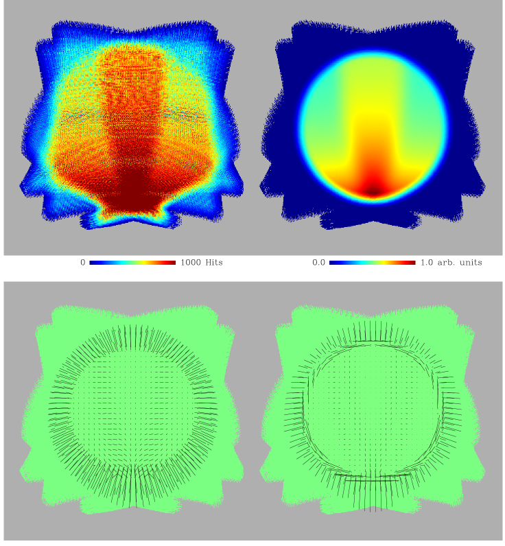
Figure 7: Inverse-variance weight functions used for power spectrum estimation for one of the southern fields. For the noise properties of our simulated data, the hit-map shown in the top left panel closely approximates the inverse-variance map. This map is heavily smoothed and apodized at the boundary of the map to produce the spin-0 weight function shown in the top right panel. The spin-1 and spin-2 weight functions, $\eth W$ and $\eth\eth W$, are shown (as vector fields) in the bottom left and right-hand panels respectively.

5 Results from simulations

The map-making and power spectrum estimation procedures described above have been applied to each of our simulated datasets treating each of our four observing fields independently. For any given simulation set, we have 50 Monte-Carlo simulations so we can estimate the uncertainties on the band-powers measured from each field. For each realisation, we can then combine our measurements from the four fields using inverse-variance weights to produce a final single estimate of the power spectrum for each realisation. When presenting our results below, in all cases, we plot the mean of these final estimates. For our reference simulation, and for the $1/f$ noise systematics, the error-bars plotted are calculated from the scatter among the realisations and are those appropriate for a single realisation. When investigating the $B$-mode bias from systematics, we plot the results from signal-only simulations and the error-bars plotted are the standard error on the mean. For some of the noise-related systematics, we will also examine the impact of modulation in the map domain where the effects are already clear.

5.1 Reference simulation

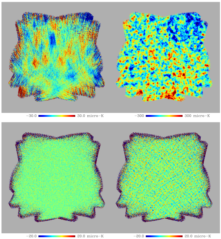
Figure 8: Sample maps constructed from simulated time-stream containing noise only (left panels) and both signal and noise (right panels). Temperature maps are shown in the top panel and $U$-polarization maps are shown in the bottom panels. These maps are for one of our reference simulations with no explicit modulation scheme and no systematics included. Note the striping in the noise-only $T$ map which is completely absent from the $U$ maps due to differencing of detector pairs before map-making.

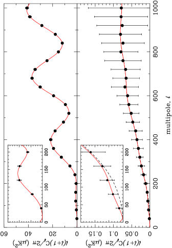
Figure 9: Mean recovered $E$-mode (top) and $B$-mode (bottom) power spectra for the reference simulations without explicit modulation. The errors plotted are those appropriate for a single realisation. The input CMB power spectra used to create the signal component of the simulations are shown as the red curves. In the bottom panel the total $B$-mode input signal (including lensing) for a tensor-to-scalar ratio of $r=0.026$ is shown as the red curve and the $B$-mode signal due to lensing alone is shown as the dashed curve. The $\ell<200$ multipole range is shown in detail in the inset plots.

To provide a reference for the results which follow, in Figs. 8 and 9 we show the results from our suite of simulations with no explicit modulation and with no systematics included. In Fig. 8 we plot examples of the reconstructed noise-only and signal-plus-noise $T$ and $U$ Stokes parameter maps (the reconstructed $Q$ maps – not shown – are qualitatively similar to $U$). The raw collecting power of an experiment like C_ℓOVER  is apparent from the top two panels in this figure. Although the noise $T$ map shown in the top-left panel is clearly dominated by striping due to the correlated noise from the atmosphere, only signal is apparent in the signal-plus-noise map shown in the top-right panel. (In fact, the noise contribution to the $T$ signal-plus-noise map is significant, particularly on large scales, and so would need to be accounted for when measuring the temperature power spectrum.) Conversely, the $U$ noise map is dominated by white noise; the correlated component of the atmosphere has been removed completely from the polarization time-streams (as has the $T$ sky signal) by differencing detector pairs before map-making.

Figure 9 shows the mean recovered $E$- and $B$-mode power spectra from our reference simulations for the case of no explicit modulation. Here, we see that our analysis is unbiased and recovers the input polarization power spectra correctly. For an input tensor-to-scalar ratio of $r=0.026$, we recover a detection of $B$-modes in excess of the lensing signal of $1.54\sigma$. (We argue in Section 6.3 that this is an under-estimate of the detection significance by around 10 per cent due to our ignoring small anti-correlations between the errors in adjacent band-powers.)

The corresponding plots for the stepped and continuously rotating HWP are very similar apart from the reconstructed polarization maps at the very edges of the fields where a modulation scheme increases the ability to decompose into the $Q$ and $U$ Stokes parameters. Since the edges of the field are excluded in our power spectrum analysis in any case (see Fig. 7), we find that the performance (in terms of $C_{\ell}$ errors) of all three types of experiments which we have considered is qualitatively the same in the absence of systematic effects. Note that for all the systematics we have considered, the effects on the recovery of the $E$-mode spectrum is negligible and so, in the following sections, we plot only the recovered $B$-mode power spectra which are the main focus of this paper.

5.2 $1/f$ detector noise

Figure 10 shows the recovered noise-only maps from a simulation containing a correlated $1/f$ detector noise component with a knee frequency of $f_{\rm knee}=0.1$ Hz. In this figure, we have plotted the noise-only maps from the three types of experiment we have considered: no modulation; a HWP which is stepped by 20^∘ at the end of each azimuth scan; and a HWP continuously rotating at $3$ Hz. The impact of modulation on $1/f$ detector noise is clear from this plot – as described in Section 3.7, the continuously rotating HWP shifts the polarization band in frequency away from the $1/f$ detector noise leaving only white noise in the resulting map. A stepped HWP, on the other hand, does not mitigate $1/f$ detector noise in this way and so noise striping is apparent in the middle panel of Fig. 10.

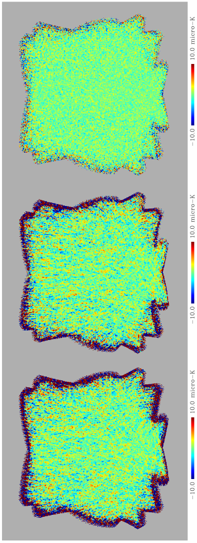
Figure 10: Sample noise-only $U$-maps from simulations containing a $1/f$ component correlated to the detector noise

. For display purposes only, the maps have been smoothed with a Gaussian with a FWHM of 7 arcmin. In the case where explicit modulation is either absent (left panel) or slow (stepped HWP; middle panel), the $1/f$ noise results in faint residual stripes in the polarization maps. In the case of a continuously rotating HWP, the polarization signal is modulated away from the low frequency $1/f$ resulting in white-noise behaviour in the polarization map (right panel).

The $B$-mode power spectra measured from our signal-plus-noise simulations including $1/f$ detector noise are shown in Fig. 11 (again for $f_{\rm knee}=0.1$ Hz) where we show the results from all three types of experiment.

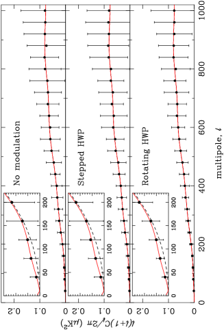
Figure 11: Recovered $B$-mode power spectra for the simulations including a correlated $1/f$ component to the detector noise with $f_{\rm knee}=0.1$ Hz for no modulation (top), a stepped HWP (middle) and a HWP continuously rotating at 3 Hz (bottom). See Table 1 for the significances with which each experiment detects the input signals.

Examination of the figure suggests that the presence of a $1/f$ component in the detector noise leads to a significant degradation in the ability of the unmodulated and stepped-HWP experiments to recover the input $B$-mode signal. This degradation happens at all multipoles but is particularly acute on the largest scales ($\ell<200$) where the primordial $B$-mode signal resides. The marginal detection of primordial $B$-modes (for $r=0.026$) which we saw in our reference simulation (Fig. 9) is now completely destroyed by the presence of the $1/f$ correlated detector noise. Furthermore, note that our analysis of the simulated data sets is optimistic in the sense that we have assumed that any correlated noise can be modelled accurately – that is, our noise-only simulations, which we use to measure the noise bias, are generated from the same model noise power spectrum used to generate the noise component in our signal-plus-noise simulations. (This is the reason that our recovered spectra are unbiased.) However, for the analysis of a real experiment, the noise properties need to be measured from the real data and there are uncertainties and approximations inherent in this process. Any correlated detector noise encountered in a real experiment is unlikely to be understood to the level which we have assumed in our analysis and so will likely result not only in the increased uncertainties we have demonstrated here but also in a biased result at low multipoles. Estimating cross-spectra between maps made from subsets of detectors for which the $1/f$ detector noise is measured to be uncorrelated is a simple way to avoid this noise bias issue, at the expense of a small increase in the error-bars (Hinshaw et al., 2003).

The results from the simulations where we have continuously modulated the polarization signal recover the input $B$-mode signal to the same precision that we saw with our reference simulation – our marginal detection of $r=0.026$ is retained even in the presence of the correlated detector noise. In Section 6.1 and Table 1 we show quantitatively that, for a detector knee frequency of $0.1$ Hz, the significance with which the continuously modulated experiment detects the primordial $B$-mode signal is roughly twice that found for the un-modulated and stepped-HWP experiments. Also detailed in Table 1 are the results from our $1/f$ noise simulations with knee frequencies of $0.05$ and $0.01$ Hz. We see, as expected, that the impact of fast modulation is less for a lower knee frequency — for $f_{\rm knee}=0.05$, rapid modulation still significantly out-performs the un-modulated and stepped-HWP experiments while for $f_{\rm knee}=0.01$ Hz, there is essentially no difference between the performance of the three types of experiment.

Note that, in the case of rapid modulation, because the polarization signal is moved completely away from the $1/f$ frequency regime, the recovered spectra should be immune to the issues of mis-estimation or poor knowledge of the noise power spectrum at low frequencies mentioned above. Although detector $1/f$ noise can be mitigated by other methods (e.g. using a more sophisticated map-maker; Sutton et al. 2009), these usually require accurate knowledge of the low-frequency noise spectrum unlike the hardware approach of fast modulation.

5.3 Polarized atmospheric $1/f$

In contrast to the addition of $1/f$ detector noise, which can be successfully dealt with by rapid modulation, all three types of experiment are degraded similarly by polarized low-frequency noise in the atmosphere. In particular, the errors at low multipoles are inflated by a large factor since the large amount of polarized atmosphere which we have input to the simulations swamps the input $B$-mode signal for $r=0.026$. We stress that the levels of polarized atmosphere we have used in these simulations were deliberately chosen to demonstrate the point that modulation does not help and the levels are certainly pessimistic.

5.4 Calibration errors

The power spectra recovered from signal-only simulations where we introduced random gain errors (constant in time) across the focal plane, or 1 per cent systematic A/B gain mis-matches between the two detectors within each pixel are shown in Fig. 12. In both cases, we see a clear bias in the recovered $B$-mode signal in the absence of fast modulation, but the bias is mitigated entirely by the presence of a HWP rotating at 3 Hz. The bias is also mitigated to some degree by the stepped HWP but not completely. In our simulations, the bias is generally larger for the case of random gain errors since the variance (across the focal plane) of the gain mismatches is twice as large in the former case. For our simulations where we allowed detector gains to drift over the course of a two-hour observation, we found a similarly behaved $B$-mode bias to those shown in Fig. 12 but with a smaller magnitude (due to the two-hour drifts averaging down over the eight-hour observation).

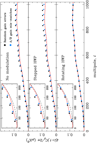
Figure 12: Mean recovered $B$-mode power spectra for the simulations including random gain errors across the focal plane (black points) or systematic 1 per cent A/B gain mis-matches between detector pairs (blue points) for no modulation (top), a stepped HWP (middle) and a continuously rotating HWP (bottom). These spectra are measured from our suite of signal-only simulations. Our simulations containing both signal and noise exhibit the same biased recovery for the no-modulation and stepped-HWP cases. The presence of a fast modulation scheme (bottom panel) mitigates entirely the bias caused by these gain mis-matches. The standard errors in these mean recovered spectra are smaller than the plotted symbols.

A mis-match between the gains of the two detectors within a pixel corresponds to a $T\rightarrow Q$ leakage in the detector basis. The projection of this instrumental polarization onto the sky will therefore be suppressed if a wide range of sensitivity directions $\phi_{i}$ contribute to each sky pixel, as is the case for fast modulation. Note that in the case of a stepped HWP, one should be careful to design the stepping strategy in such a way that it does not undo some of the effect of sky rotation. During our analysis, we have found that the performance of a stepped HWP in mitigating systematic effects can depend critically on the direction, magnitude and frequency of the HWP step applied. In fact, for some set-ups we have investigated, a stepped HWP actually worsened the performance in comparison to the no modulation case due to interactions between the scan strategy and HWP stepping strategy. However, the results plotted in Fig. 12 for the stepped HWP case are for a HWP step of $20^{\circ}$ between each azimuth scan which is large and frequent enough to ensure that such interactions between the stepping strategy and the scan strategy are sub-dominant.

5.5 Mis-estimated polarization angles

The next set of systematics we have considered concern a mis-estimation of both the detector orientation angles (i.e. the direction of linear polarization to which each detector is sensitive to) and, for the case where a HWP is employed, a mis-estimation of the HWP orientation. We have performed simulations including both a random scatter (with an RMS of $0.5^{\circ}$) and a systematic offset of $0.5^{\circ}$ in the simulated detector and HWP angles. Note that for the systematic offset in the detector angles, the same offset is applied to all detectors. For both the detector angles and the HWP, the offset introduced corresponds to a systematic error in the estimation of the global polarization coordinate frame of the experiment and the effects are therefore degenerate.

For the simulations which included a random scatter in the angles (both detector angles and HWP orientation), we found neither a bias in the recovered $B$-mode power spectra, nor a degradation in the error-bars from the simulations containing both signal and noise. Following the discussion in Section 3.6, common errors in the detector angles for the pair of detectors in a single focal-plane pixel give rise to a rotation of the polarization sensitivity direction of the pixel, while differential errors reduce the polarization efficiency. For a typical differential scatter of $\sqrt{2}\times 0.5^{\circ}$, the reduction in the polarization efficiency ($\sim 10^{-4}$) is negligible. For a given pixel on the sky, the impact of the polarization rotation is suppressed by $\sqrt{N_{\mathrm{sample}}}$, where $N_{\mathrm{sample}}$ is the total number of samples contributing to that pixel with independent errors in the angles. The combination of a large number of detectors and, in the case of random HWP angle errors, their assumed short correlation time in our simulations renders the effect of small and random scatter in the angles negligible.

The results from simulations which included a systematic error in the angles are shown in Fig. 13, where we plot the recovered $B$-mode power spectrum from our signal-only simulations. In contrast to the simulations with random scatter, there is a clear mixing between $E$ and $B$ due to the systematic mis-calibration of the polarization coordinate reference system of the instrument. A global mis-estimation of the polarization direction by an angle $\psi$ in the reconstructed maps leads to spurious $B$-modes with

$$C_{\ell}^{B}=\sin^{2}(2\psi)C_{\ell}^{E}\approx 4\psi^{2}C_{\ell}^{E}.$$ (30)

Note that in Fig. 13, we show the results from the detector angle systematic only for the case of the non-modulated experiment but the plot is identical for both the stepped and continuously rotating HWP – polarization modulation cannot mitigate a mis-calibration of detector angles. The fact that the mixing apparent in Fig. 13 is greater for the HWP mis-calibration is simply because rotating the waveplate by $\psi$ rotates the polarization direction by $2\psi$. Although the spurious $B$-mode power is most noticeable at high multipoles, where $\ell(\ell+1)C_{\ell}^{E}$ is largest, it is also present on large scales and, as is clear from the plot, would bias a measurement of the $B$-mode spectrum at all multipoles.

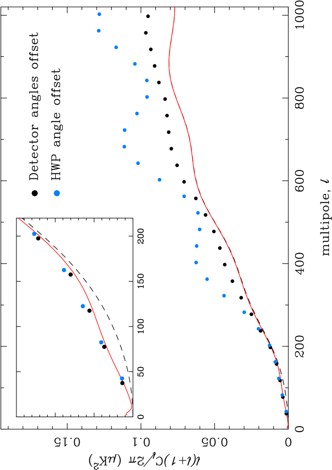
Figure 13: Mean recovered $B$-mode power spectra for the signal-only simulations including mis-estimated detector polarization sensitivity angles (black points) and mis-estimated HWP angles (blue points) where the angles have been systematically offset by 0.5^∘ in both cases. The standard errors in these mean recovered spectra are smaller than the plotted symbols.

5.6 Mis-estimated time-constants

The power spectra measured from simulations which included random and systematic errors in the detector time-constants displayed neither a bias, nor a degradation in error-bars. This was to be expected for the slow scan speed and extremely fast time-constants we have considered in this analysis – the response function of the C_ℓOVER  detectors is effectively phase-preserving with zero attenuation in the frequency band which contains the sky-signal in our simulations. Note that this would not necessarily have been the case had we considered a much faster scan speed or more rapid polarization modulation.

5.7 Pointing errors

Our analysis of simulations where we have introduced a jitter in the pointing and/or an overall wander in the pointing suggest that these systematics have only a very small effect on the recovered $B$-mode power spectra, at least for the levels which we have considered (i.e. a $30$ arcsec random jitter in the pointing and/or an overall wander of the pointing by $1$ arcmin over the course of a two-hour observation). The only observed effect was a slight suppression of the recovered $B$-mode signal at high multipoles consistent with a slight smearing of the effective beam. We note however that the effect we observed was extremely small and was only noticeable in our signal-only simulations. For our simulations containing noise, the effect was completely swamped by the errors due to random noise.

In principle, pointing errors can also lead to leakage from $E$ to $B$ (Hu, Hedman & Zaldariagga, 2003; O’Dea, Challinor & Johnson, 2007). In Appendix A we develop a toy-model for the leakage expected from random pointing jitter in the case of a scan/modulation strategy that produces a uniform spread of polarization sensitivity directions in each sky pixel (such as by fast modulating with a HWP). The result is a white-noise spectrum of $B$-modes but, for the simulation parameters adopted here, the effect is very small – less than $1$ per cent of the $B$-mode power induced by weak gravitational lensing on large scales.

5.8 Differential transmittance in the HWP

The power spectra reconstructed from our simulations which included a 2 per cent differential transmittance in the HWP exhibited no degradation in the accuracy of the recovered $B$-mode signal — even the relatively simple recipe which we have used to remove the HWP-synchronous signals from the time-stream (see Section 4.1) appears sufficient to recover the $B$-mode signal to the same accuracy as was seen in our reference simulations. (We quantify this statement in the next section where we estimate the detection significances with which the different simulations detect the $E$ and $B$-mode signals). As mentioned in Section 3.7, the recovered polarization signal is mis-calibrated by $\sim 2$ per cent in amplitude ($4$ per cent in power). Compared to the random noise however, this mis-calibration is a small effect and is easily dealt with during, e.g. a cosmological parameter analysis by marginalising over it.

Note that no prior information on the level of differential transmittance was used during our analysis of the data. Our technique for removing the HWP-synchronous signals is a blind one in this sense and should work equally well for other HWP-systematic effects that result in spurious signals at harmonics of the HWP rotation frequency, $f_{\lambda}$.

6 Discussion

6.1 Controlling systematics with polarization modulation

The main goal of the analysis presented in this paper is to demonstrate and quantify with simulations the impact of two types of polarization modulation (slow modulation using a stepped HWP and rapid modulation with a continuously rotating HWP) on the science return of upcoming CMB $B$-mode experiments in the presence of various systematic effects. Although our list of included systematics is not an exhaustive one (in particular, we are still investigating the case of imperfect optics), we are nevertheless in a position to draw some rather general conclusions regarding the usefulness of modulation in mitigating systematics. It is, of course, important to bear in mind that we have only considered two examples of a HWP-related systematic effect (imperfect HWP angles and differential transmittance in the plate). The are many more possible effects which will need to be well understood and strictly controlled if fast polarization modulation with HWPs is to realise its potential.

(i) Systematics mitigated by modulation

• Correlated $1/f$ detector noise: As expected by the general reasoning of Section 3.7, and further borne out by our results from simulations, rapid polarization modulation is extremely powerful at mitigating a correlated $1/f$ component in the detector noise. Any such $1/f$ component is not mitigated by a HWP operating in stepped mode.

• Calibration errors: Our results demonstrate that fast modulation is also useful for mitigating against possible calibration errors since it greatly increases the range of directions over which sky polarization is measured in a given pixel. For example, the clear bias introduced in our simulations by random gain drifts or systematic mis-calibrations between detectors was mitigated entirely by the HWP continuously rotating at $3$ Hz. This bias was also partly (but not completely) mitigated by stepping the HWP by 20^∘ between each of our azimuth scans. For some stepping strategies we have investigated, the bias actually increased — a poor choice of stepping strategy can actually be worse than having no modulation because of interactions between the sky rotation and the HWP orientations.

Table 1: Detection significances (in units of $\sigma$) for our reference simulations, for our simulations with $1/f$ noise systematics and for our simulations with a 2 per cent differential transmittance in the HWP. Also included for comparison are the predicted detection significances from a Fisher matrix analysis of the power spectrum errors (see Section 6.3) and from the simulations containing isotropic and uniform Gaussian noise (see text). The rightmost column displays the significance of the detection of the $B$-mode signal in excess of the lensing signal which corresponds directly to the significance with which each simulation detects the input tensor-to-scalar ratio of $r=0.026$.

Simulation	Modulation	$E$-mode	$B$-mode	$r=0.026$
Fisher predictions	—	$128.6$	$10.24$	$1.90$
Uniform noise	—	$126.4$	$10.30$	$1.45$
Reference simulation	None	$127.8$	$10.41$	$1.54$
	Stepped HWP	$130.1$	$10.11$	$1.41$
	Rotating HWP	$127.7$	$10.72$	$1.45$
$1/f$ detector noise	None	$124.2$	$7.29$	$0.83$
($f_{\rm knee}=0.1$ Hz)	Stepped HWP	$124.6$	$7.09$	$0.79$
	Rotating HWP	$126.8$	$9.96$	$1.47$
$1/f$ detector noise	None	$125.1$	$8.61$	$0.95$
($f_{\rm knee}=0.05$ Hz)	Stepped HWP	$127.5$	$8.59$	$1.14$
	Rotating HWP	$125.6$	$10.31$	$1.45$
$1/f$ detector noise	None	$126.8$	$9.78$	$1.30$
($f_{\rm knee}=0.01$ Hz)	Stepped HWP	$128.0$	$9.99$	$1.44$
	Rotating HWP	$127.1$	$10.28$	$1.40$
Polarized atmosphere	None	$122.9$	$6.86$	$0.12$
	Stepped HWP	$124.9$	$6.99$	$0.10$
	Rotating HWP	$126.0$	$8.24$	$0.21$
Differential transmittance	Rotating HWP	$127.6$	$10.92$	$1.59$

(ii) Systematics not mitigated by modulation

• Polarized $1/f$ atmosphere: No amount of modulation (rapid or slow) will mitigate a polarized $1/f$ component in the atmosphere. The results from our simulations containing polarized atmosphere are summarised in Table 1.

• Pointing errors: For our simulations which included pointing errors, the effect on the recovered $B$-mode power spectra was extremely small and was equivalent to a slight smoothing of the effective beam. Although the same amount of smoothing was observed in all the simulations (and so the effect is not mitigated by polarization modulation), the effect is negligible for the sensitivities and beam sizes considered here. The further leakage of $E$-mode power into $B$ modes due to pointing errors was, as expected (see Appendix A) unobservably small in our simulations.

• Mis-calibration of polarization angles: A polarization modulation scheme does not mitigate a systematic error in the calibration of the polarization sensitivity directions. Experiments using a HWP will require precise and accurate measurements of the HWP angle at any given time to avoid the $E\rightarrow B$ mixing apparent in Fig. 13.

Our results are in broad agreement with those of a similar study by MacTavish et al. (2008) who based their analysis on signal-only simulations of the SPIDER  experiment. Both MacTavish et al. (2008) and this study find that polarization modulation with a continuously rotating HWP is extremely effective in mitigating the effects of $1/f$ detector noise but that, in the presence of significant $1/f$ noise, the analysis of an experiment where modulation is either absent or slow will require near-optimal map-making techniques. In addition, both studies find that the effect of small and random pointing errors on the science return of upcoming $B$-mode experiments is negligible given the experimental sensitivities. The two analyses also find that the effect of random errors (with $\sim 0.5^{\circ}$ RMS) in the detector polarization sensitivity angles is negligible but that the global polarization coordinate frame of the experiment needs to be measured carefully — MacTavish et al. (2008) quote a required accuracy of $<0.25^{\circ}$ for SPIDER  which is consistent with the requirement for an unbiased measurement of the $B$-mode signal (for $r=0.026$) at $\ell<300$ with C_ℓOVER. Finally, both studies suggest that, in the absence of fast modulation, relative gain errors will also need to be controlled to the $<1$ per cent level (although, in this paper, we have demonstrated that such gain errors are almost entirely mitigated using a fast modulation scheme; see Fig. 12).

In Table 1, we quantify the impact of modulation on the $1/f$ noise systematics we have considered in this work by considering the significances with which we detect the $E$-mode and $B$-mode signals. For comparison, the detection significances in the presence of a 2 per cent differential transmittance in the HWP are also presented. To calculate the total significance of the detection we compute the Fisher error on the amplitude of a fiducial spectrum,

$$\frac{S}{N}=\left(\sum_{bb^{\prime}}P_{b}^{\rm fid}{\rm cov}^{-1}_{bb^{\prime}}P_{b^{\prime}}^{\rm fid}\right)^{1/2},$$ (31)

where ${\rm cov}^{-1}_{bb^{\prime}}$ is the inverse of the band-power covariance matrix for the given spectrum. For the total significance of a detection of $E$ or $B$-modes, the fiducial band-powers are simply the binned input power spectra. In order to estimate the significance of a detection of primordial $B$-modes, we subtract the lensing contribution from the input $B$-mode power spectra. Because the primordial $B$-mode power spectrum is directly proportional to the tensor-to-scalar ratio, $r$, the significance with which we detect the $B$-mode signal in excess of the lensing signal translates directly to a significance for the detection of our input tensor-to-scalar ratio of $r=0.026$. When analysing the results of the simulations, we approximate ${\rm cov}^{-1}_{bb^{\prime}}\approx\delta_{bb^{\prime}}/\sigma_{b}^{2}$ since we are unable to estimate the off-diagonal elements from our small number of realisations (50) in each simulation set. We know from a Fisher-based analysis (see Section 6.3), the results of which are also reported in Table 1, that neighbouring band-powers on the largest scales are, in fact, $\sim 10$ per cent anti-correlated, and the diagonal approximation therefore underestimates the detection significance by $\sim 10$ per cent. For consistency, the numbers quoted for the Fisher analysis ignore the off-diagonal elements of the covariance matrix. Including the correlations increases the $E$-mode significance to $144.6$ (from $128.6$), the total $B$-mode significance to $11.57$ (from $10.24$) and the primordial $B$-mode significance to $2.04$ (from $1.90$).

In comparing the entries in Table 1 one should keep in mind that the significances reported for the simulations are subject to a Monte-Carlo error due to the finite number ($N_{\mathrm{sim}}=50$) of simulations used to estimate the band-power errors. Approximating the band-powers as uncorrelated and Gaussian distributed, the sampling error in our estimates of the $S/N$ is

$$\Delta(S/N)\approx\frac{1}{S/N}\frac{1}{\sqrt{2N_{\mathrm{sim}}}}\left[\sum_{b}\left(\frac{P_{b}^{\mathrm{fid}}}{\sigma_{b}}\right)^{4}\right]^{1/2}.$$ (32)

For the reference simulation, this gives an error of $0.15$ in the significance of a detection of $r$ and $0.22$ in the significance of the total $B$-mode spectrum. The size of these errors likely explain the apparent anomalies that rotating the HWP degrades the detection of $r$ in the reference simulation, and that adding $1/f$ detector noise improves the detection of $r$ over the reference simulation for the case of a rotating HWP.

Also included in Table 1 is the performance of our experiment as estimated from a set of simple map-based simulations where we have injected uniform and isotropic white noise into signal-only $T$, $Q$ and $U$ maps directly. In these simulations, and also for the Fisher analysis, the white-noise levels were chosen to match the noise levels in our main analysis and so they have identical raw sensitivity to the time-stream simulations but with perfectly behaved noise properties. The broad agreement between our full time-stream simulations and these simple map-based simulations suggests that the anisotropic noise distribution introduced by the C_ℓOVER  scan strategy does not have a large impact on the performance of the experiment. This agreement also suggests that the slightly poorer performance of the simulations in recovering the $r=0.026$ primordial $B$-mode signal as compared to the Fisher predictions is due to the sub-optimal performance on large scales of the (pure) pseudo-$C_{\ell}$ estimator we have used.

6.2 Importance of combining data from multiple detectors

For all of our analyses up to this point, in order to remove the correlated $1/f$ atmospheric noise from the polarization analysis, we have differenced detector pairs before map-making. However, as mentioned in Section 3.7, for the case of a continuously modulated experiment, it is possible to measure all three Stokes parameters from a single detector in isolation. Here, we argue that this may be a poor choice of analysis technique in the presence of a highly correlated and common-mode systematic such as atmospheric $1/f$, at least when one employs real-space demodulation techniques such as those that we have used in this analysis. The key point to appreciate here is that, even with a rapid modulation scheme, and for an ideal experiment, it is impossible to separate completely the temperature and polarization signals in real space using only a single detector. In contrast, the technique of detector differencing achieves this complete separation of the temperature and polarization signals (again for the case of an ideal experiment). Note that this is true even in the signal-only case. Consider again the modulated signal, in the absence of noise, from a single detector sensitive to a single polarization:

$$d_{i}=\left[T(\theta)+Q(\theta)\cos(2\phi_{i})+U(\theta)\sin(2\phi_{i})\right]/2.$$ (33)

If for each observed data point, $d_{i}$, the true sky signals, $T$, $Q$ and $U$ are different (as is the case for a scanning experiment), there is clearly no way to recover the true values of $T$, $Q$ and $U$ at each point in time. The approximation that one must make in order to demodulate the data in real space goes to the very heart of map-making – that the true continuously varying sky signal can be approximated as a pixelised distribution where $T$, $Q$ and $U$ are taken to be constant within each map-pixel. Armed with this assumption, all three Stokes parameters can be reconstructed from a single detector time-stream using a generalisation of equation (25):

$$\left(\begin{array}[]{c}T\\ Q\\ U\end{array}\right)=2\,{\mathsf{M}}^{-1}\cdot\left(\begin{array}[]{c}\langle d_{i}\rangle\\ \langle\cos(2\phi_{i})d_{i}\rangle\\ \langle\sin(2\phi_{i})d_{i}\rangle\\ \end{array}\right).$$ (34)

where the decorrelation matrix, ${\mathsf{M}}$ is now given by

$${\mathsf{M}}=\left(\begin{array}[]{ccc}\!\!\!1&\!\!\!\langle\cos(2\phi_{i})\rangle&\!\!\!\!\!\langle\sin(2\phi_{i})\rangle\\ \!\!\!\langle\cos(2\phi_{i})\rangle&\!\!\!\langle\cos^{2}(2\phi_{i})\rangle&\!\!\!\!\!\langle\cos(2\phi_{i})\sin(2\phi_{i})\rangle\\ \!\!\!\langle\sin(2\phi_{i})\rangle&\!\!\!\langle\cos(2\phi_{i})\sin(2\phi_{i})\rangle&\!\!\!\!\!\langle\sin^{2}(2\phi_{i})\rangle\\ \end{array}\!\!\!\!\right).$$ (35)

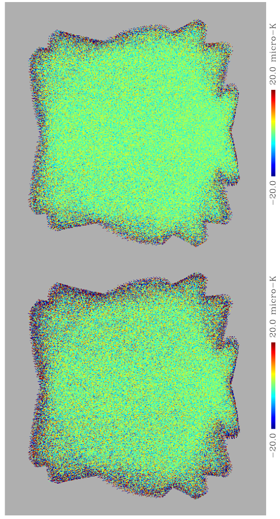
Figure 14: Recovered noise only $U$-polarization maps from one of our reference simulations with continuous modulation. The map on the left is reconstructed from demodulated single detector “pure” $U$ time streams and has not used information from multiple detectors to separate the $T$ and polarization signals. The map on the right is made from demodulated detector-pair “pure” $U$ time-streams and explicitly combines information from the two detectors within each pixel to separate $T$ from $Q/U$. Although striping is absent from both maps, the white-noise level in the detector-differenced map is reduced compared to that made using the non-differencing analysis.

If, on the other hand, the data from different detectors are combined (e.g. when detector differencing is used), the situation is different – because the two detectors within a pixel observe exactly the same un-polarized component of the sky signal at exactly the same time, differencing the detectors removes the $T$ signal completely without any assumptions regarding the scale over which the true sky signal is constant. In this case, the decorrelation of $Q$ and $U$ using equation (25) still requires an assumption regarding the constancy of the $Q$ and $U$ signals over the scale of a map-pixel but now the much larger temperature signal has been removed from the polarization analysis completely.

Now, if in addition to the sky signal, we have a common-mode time-varying systematic such as an un-polarized $1/f$ component in the atmosphere, this contaminant will again be removed entirely with the detector differencing technique (as long as it is completely correlated between the two detectors) whilst it will introduce a further approximation into any attempt to decorrelate all three Stokes parameters from a single detector time-stream using equation (34).

To illustrate this point, and to stress the importance of combining data from multiple detectors, we have re-analysed the simulated data from our set of continuously modulated reference simulations but now we perform the demodulation at the time-stream level for either single detectors or single detector-pairs in isolation. Firstly, we demodulate each detector time-stream individually using equation (34) but now the averaging is performed over short segments in time rather than over all data falling within a map-pixel. This procedure results in “pure” $T$, $Q$ and $U$ time-streams for each detector but at a reduced data rate determined by the number of data samples over which the averaging of equation (34) is performed. For our second analysis, we first difference each detector pair and then demodulate the differenced time-streams using equation (25), again applied over short segments of time, resulting in “pure” $Q$ and $U$ time-streams for each detector pair, once again at a reduced data rate. Maps of the $Q$ and $U$ Stokes parameters are then constructed by simple binning of the demodulated $Q$ and $U$ time-streams from all detectors or detector pairs. In the case where detector pairs are differenced, we are explicitly combining information from multiple detectors to separate the temperature and polarization signals whilst when we do not difference, we are attempting to separate the $T$ and $Q/U$ signals present in detector time-stream in isolation.

The results of these tests are shown in Figs. 14 and 15. Figure 14 shows the noise-only $U$-polarization maps recovered using the two different analysis techniques. Although striping from the atmospheric fluctuations is not present in either of the maps, the extra uncertainty introduced when one attempts to separate the $T$ and $Q/U$ signals from individual detectors in isolation clearly results in an increased white noise level in the polarization maps. This results in a degradation factor of $\sim 2$ in the resulting measurements of the $B$-mode power spectrum on all angular scales (Fig. 15) with a corresponding degradation in the detection significances for both a measurement of the total $B$-mode signal and for a detection of $r=0.026$ (Table 2). These results are in excellent agreement with those of Sutton et al. (2009) who found it necessary to apply optimal mapping techniques to rapidly modulated single-detector time-streams in the presence of $1/f$ atmospheric noise.

We emphasise that the results presented in Fig. 15 and in Table 2 for the case where we have analysed single detectors in isolation would likely be improved if the Fourier domain filtering used in Johnson et al. (2007) was implemented. We are currently working to integrate this step into our algorithm, and we expect to report the subsequent improvement in future publications.

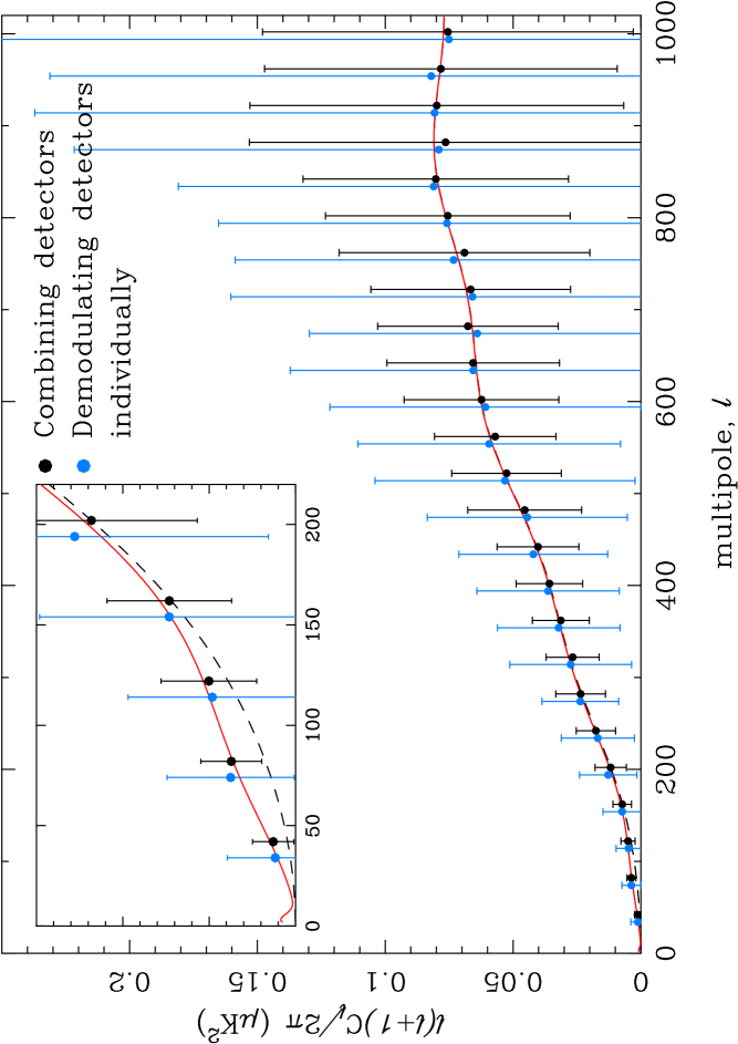
Figure 15: Comparison between the $B$-mode power spectra recovered using an analysis based on differencing detector pairs (black points) and one based on demodulating each detector individually (blue points). In the presence of a time-varying common-mode systematic, such as the $1/f$ atmospheric noise we have considered here, the analysis based on detector differencing is far superior to the analysis based on demodulating each detector individually.

Table 2: Detection significances (in units of $\sigma$) from the analysis of identical simulated data with a HWP rotating continuously at $3$ Hz. The first analysis is based on detector differencing, the second based on demodulation of individual detectors in isolation.

Analysis	$E$-mode	$B$-mode	$r=0.026$
Detector differencing	$132.9$	$10.14$	$1.43$
Demodulation	$123.4$	$5.11$	$0.68$

6.3 Comparison of simulated and predicted C_ℓOVER  performance

It is common practice to make predictions of the performance of upcoming experiments using a Fisher-matrix analysis which attempts to predict the achievable errors on, for example, power spectra or cosmological parameters under some simplifying assumptions. Generally these assumptions will include uniform coverage of the observing fields and uncorrelated Gaussian noise resulting in an isotropic and uniform white-noise distribution across the observing field. In contrast, the work described in this paper has made use of a detailed simulation pipeline which we have created for the C_ℓOVER  experiment. Our simulation pipeline includes the C_ℓOVER  focal-plane designs as well as a realistic scan strategy appropriate for observing the four chosen C_ℓOVER  fields from the telescope site in Chile. In addition we have employed a detailed model of the TES detector noise properties and responsivity, and $1/f$ atmospheric noise correlated across the focal-plane array. Moreover, our errors are calculated using a Monte-Carlo analysis and so should automatically include any effects due to correlations between map pixels etc. An interesting exercise therefore is to compare the expected errors from a Fisher-matrix analysis to those obtained from our simulation analysis.

The polarization band-power Fisher matrix is (e.g. Tegmark & de Oliveira-Costa 2001)

$$\mathrm{cov}^{-1}_{(bP)(bP)^{\prime}}=\frac{1}{2}\mathrm{tr}\left(\textbf{{C}}^{-1}\frac{\partial\textbf{{C}}}{\partial\mathcal{C}_{b}^{P}}\textbf{{C}}^{-1}\frac{\partial\textbf{{C}}}{\partial\mathcal{C}_{b^{\prime}}^{P^{\prime}}}\right)$$ (36)

where $P$ and $P^{\prime}$ are $E$ or $B$, and $b$ labels the bandpower. Here, C is the covariance matrix of the noisy Stokes maps and $\mathcal{C}_{b}^{P}$ are bandpowers of $\ell(\ell+1)C_{\ell}^{P}/(2\pi)$. We analyse a single circular field with area equal to that retained in the pseudo-$C_{\ell}$ analysis described in Section 4.2, and multiply the Fisher matrix by four to account for the number of fields observed (which are thus assumed to be fully independent). We ignore inhomogeneity of the noise in the maps so that our problem has azimuthal symmetry about the field centre. This allows us to work in a basis where the data is Fourier transformed in azimuth and the covariance matrix becomes block diagonal, thus speeding up the computation of the Fisher matrix considerably. The Fisher matrix takes full account of band-power correlations (both between $b$ and polarization type) and the effect of ambiguities in isolating $E$ and $B$-modes given the survey geometry. We deal with power on scales larger than the survey by including a junk band-power for each of $E$ and $B$ whose contribution to $\mathrm{cov}_{(bP)(bP)^{\prime}}$ we remove before computing detection significances.

The comparison between the predicted and simulated performance of C_ℓOVER  is shown in Fig. 16. In this plot, we also include the predicted $B$-mode errors from a naïve mode-counting argument based on the fraction of sky observed, $f_{\rm sky}$. For these estimates, we assume independent measurements of the power spectrum in bands of width $\Delta\ell$ given by

$$(\Delta C_{\ell})^{2}=\frac{2}{(2\ell+1)f_{\rm sky}\Delta\ell}(C_{\ell}+N_{\ell})^{2},$$ (37)

where $C_{\ell}$ is the band-averaged input signal and $N_{\ell}$ is the band-averaged noise. For uncorrelated and isotropic Gaussian random noise, the latter is given by $N_{\ell}=w^{-1}B_{\ell}^{-2}$ where $B_{\ell}=\exp(-\ell(\ell+1)\sigma_{B}^{2}/2)$ is the transform of the beam with $\sigma_{B}=\theta_{B}/\sqrt{8\ln 2}$ for a beam with FWHM of $\theta_{B}$. The weight $w^{-1}=\Omega_{\rm pix}\sigma^{2}_{\rm pix}$, where the pixel noise in the $Q$ and $U$ maps is

$$\sigma^{2}_{\rm pix}=\frac{({\rm NET}/\sqrt{2})^{2}\Theta^{2}}{t_{\rm obs}(N_{\rm det}/4)\Omega_{\rm pix}}.$$ (38)

Here $\Theta^{2}$ is the total observed area, $t_{\rm obs}$ is the total observation time and $\Omega_{\rm pix}$ is the pixel size. In equation (38), we have used ${\rm NET}/\sqrt{2}$ to account for the fact that a single measurement of $Q$ or $U$ requires a measurement from two detectors (or, alternatively, two measurements from a single detector) and we use $N_{\rm det}/4$ as the effective number of $Q$ and $U$ detectors.

Over most of the $\ell$ range, the agreement between the Fisher matrix predictions and the simulated performance is rather good – the only significant discrepancy is for the lowest band-power where the simulations fail to match the predicted Fisher error. This is almost certainly due to the relatively poor performance of our power spectrum estimator on the very largest scales where pseudo-$C_{\ell}$ techniques are known to be sub-optimal (compared to, for example, a maximum likelihood analysis). In terms of a detection of the total $B$-mode signal, the Fisher analysis predicts a detection for C_ℓOVER  of $\sim 12.0\sigma$. For comparison, the naïve $f_{\rm sky}$ analysis predicts a $12.4\sigma$ detection. For our assumed tensor-to-scalar ratio, the Fisher matrix analysis predicts $r=0.026\pm 0.013$ (a $2.04\sigma$ detection) and the naïve analysis yields $r=0.026\pm 0.011$ (a $2.39\sigma$ detection). Comparing to the detection significances quoted in Table 1, we see that the detections recovered from the simulations fail to match these numbers. For the case of the total $B$-mode amplitude, this discrepancy is entirely due to the fact that we are unable to measure and include in our analysis (anti-)correlations between the band-powers measured from our small number (50) of simulations – when we neglect the correlations in the Fisher matrix analysis, the Fisher prediction drops to a $10.24\sigma$ detection, in excellent agreement with our measured value from simulations. For the primordial $B$-mode signal only, the discrepancy found is also partly due to the same effect (ignoring correlations in the Fisher analysis reduces the Fisher prediction for primordial $B$-modes to $1.9\sigma$). As mentioned above, we suspect that the additional decrease in sensitivity to primordial $B$-modes seen in the simulations is due to the slightly sub-optimal performance of our implementation of the pure pseudo-$C_{\ell}$ estimator on the largest scales.

We should point out that in this work, we have made no attempt to optimise the survey strategy in light of recent instrument developments. In particular, the survey size we have adopted for these simulations was optimised for a measurement of $r=0.01$ with C_ℓOVER  when the experiment was expected to have twice the number of detectors now planned. For the instrument parameters we have adopted in this analysis (which are a fair representation of the currently envisaged experiment), the optimal survey area for a measurement of $r=0.026$ would be significantly smaller than the $\sim 1500$ deg² we have used here due to the increased noise levels from the reduced number of detectors. Alternatively, if we had assumed a larger input value of $r$, the optimal survey size would increase. Optimisation of both the survey area and the scan strategy in light of these changes in the instrument design is the subject of on-going work.

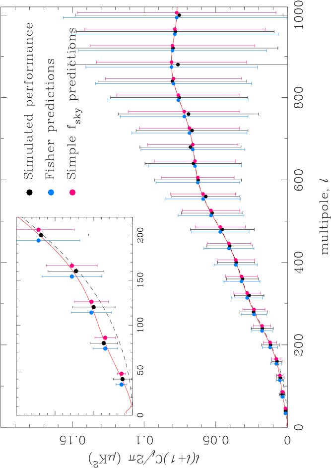
Figure 16: Comparison between the predicted performance of C_ℓOVER  as calculated using a Fisher-matrix analysis and the simulated performance from our Monte-Carlo pipeline (for our reference simulation). Also shown for comparison are the errors predicted from a naïve $f_{\rm sky}$ analysis.

There are, of course, many other sources of uncertainty which we have not yet accounted for in our simulation pipeline and so both the predicted and simulated performance numbers should be taken only as guidelines at this time. However, it is encouraging that the extra sources of uncertainty which are included in our simulation pipeline (realistic instrument parameters, a realistic scan strategy, correlated noise), in addition to any uncertainties introduced as part of our subsequent analysis of the simulated data, do not degrade the expected performance of C_ℓOVER  by a large amount.

7 Conclusions

We have performed a detailed investigation of the ability of both slow and fast polarization modulation schemes to mitigate possible systematic effects in upcoming CMB polarization experiments, targeted at measuring the $B$-mode signature of gravitational waves in the early universe. To do this we have used a simulation pipeline developed in the context of the C_ℓOVER  experiment, which includes realistic instrument and observation parameters as well as $1/f$ detector noise and $1/f$ atmospheric noise correlated across the C_ℓOVER  focal-plane array. Using this simulation tool, we have performed simulations of C_ℓOVER  operating with no explicit modulation, with a stepped HWP and with a HWP rotating continuously at $3$ Hz. We have analysed the resulting time-stream simulations using the technique of detector differencing coupled with a naïve map-making scheme, and finally have reconstructed the $E$ and $B$-mode power spectra using an implementation of the near-optimal “pure” pseudo-C_ℓ power spectrum estimator.

As expected, we find that fast modulation via a continuously rotating HWP is extremely powerful in mitigating a correlated $1/f$ component in the detector noise but that a stepped HWP is not. In addition, we have demonstrated that a polarized $1/f$ component in the atmosphere is not mitigated by any amount of modulation and if present, would need to be mitigated in the analysis using a sophisticated map-making technique. We have further verified with simulations that fast modulation is very effective in mitigating instrumental polarization that is fixed relative to the instrument basis, for example the $T\rightarrow Q$ leakage caused by systematic gain errors and mis-matches between detectors, in agreement with the conclusions of O’Dea, Challinor & Johnson (2007). We have also demonstrated that modulation does not mitigate a systematic mis-calibration of polarization angles and that these angles will need to be measured accurately in order to avoid a systematic leakage between $E$ and $B$-modes. The other systematics which we have investigated (pointing errors, mis-estimated time-constants) have a negligible impact on the recovered power spectra for the parameters adopted in our simulations.

In addition to our investigation of systematic effects, we have stressed the importance of combining data from multiple detectors and have demonstrated the superior performance of a differencing technique as opposed to one based on measuring all three Stokes parameters from single detectors in isolation. We suggest that the latter technique, although possible in the presence of rapid modulation, is likely a poor choice of analysis technique, at least in the presence of a common-mode systematic effect such as atmospheric $1/f$ noise.

Finally, we have compared the simulated performance of the C_ℓOVER  experiment with the expected performance from a simplified Fisher-matrix analysis. For all but the very lowest multipoles, where the simulations fail to match the Fisher predictions, we find excellent agreement between the predicted and simulated performance. In particular, despite the highly anisotropic noise distribution present in our simulated maps, our measurement of the total $B$-mode signal matches closely with the Fisher matrix prediction (the latter assuming isotropic noise). On the other hand, the measurement of the large scale $B$-mode signal (and thus of the tensor-to-scalar ratio, $r$) from the simulations is around 20 per cent worse than the Fisher prediction. This is almost certainly due to the sub-optimality of our power spectrum analysis on large scales. It is possible that the Fisher matrix predictions could be recovered from the simulations by using a more optimal weighting scheme in the pure pseudo-$C_{\ell}$ analysis, or, more likely, by using a maximum-likelihood $C_{\ell}$ estimator for the low multipoles.

One important class of systematic effects which we have not considered in this paper are those associated with imperfect optics. Additionally, we have considered only two effects associated with an imperfect HWP. The efficacy of fast modulation to mitigate systematic effects from imperfect optics, for example instrumental polarization due to beam mis-match, is expected to depend critically on the optical design (such as the HWP location). We are currently working to include such optical systematics in our simulation pipeline, along with a more detailed physical model of the atmosphere and models of the expected polarized foreground emission. In future work, in addition to investigating further systematic effects, we will extend our simulations to multi-frequency observations and will use these to test alternative foreground removal techniques. We will also apply the “destriping” map-making technique of Sutton et al. (2009) to our simulations to assess the relative merits of destriping in analysis as opposed to a hardware based approach for mitigating $1/f$ noise.

Appendix A $E$-$B$ leakage from pointing jitter

For the case of random pointing jitter and a scan/modulation strategy that ensures every sky pixel is visited with a wide range of polarization sensitivity directions, it is straightforward to estimate the spurious $B$-mode power that is induced from $E$-modes for a single focal-plane pixel. We work in the flat-sky approximation where directions on the sky are denoted by positions $\mn@boldsymbol{x}$ in the tangent plane. A given sky pixel $p$ receives $N_{p}$ hits with polarization sensitivity directions $\{\phi_{i}\}$, where $i=1,\ldots,N_{p}$, and assume these angles are uniformly distributed. If $d_{i}$ is the $i$th differential measurement from the detector pair contributing to pixel $p$, then we can approximate the recovered Stokes parameters in that pixel (equation 25) as

$$\hat{Q}(\mn@boldsymbol{x}_{p}) \approx \frac{2}{N_{p}}\sum_{i}d_{i}\cos(2\phi_{i})$$

$$\hat{U}(\mn@boldsymbol{x}_{p}) \approx \frac{2}{N_{p}}\sum_{i}d_{i}\sin(2\phi_{i}).$$ (39)

If the $i$th observation has a pointing error $\mn@boldsymbol{\alpha}_{i}$, then the signal contribution to $\hat{Q}(\mn@boldsymbol{x}_{p})$, for example, is

$$\hat{Q}(\mn@boldsymbol{x}_{p}) \approx \frac{2}{N_{p}}\sum_{i}\left[Q(\mn@boldsymbol{x}_{p}+\mn@boldsymbol{\alpha}_{i})\cos^{2}(2\phi_{i})\right.$$ (40)

$$\mbox{}\left.\phantom{xxxxxxx}+U(\mn@boldsymbol{x}_{p}+\mn@boldsymbol{\alpha}_{i})\sin(2\phi_{i})\cos(2\phi_{i})\right].$$

Note that here, $Q$ and $U$ are the beam-smoothed fields. Approximating the displaced Stokes parameters by a gradient approximation, we find

$$\hat{Q}(\mn@boldsymbol{x}_{p})\approx Q(\mn@boldsymbol{x}_{p})+\mn@boldsymbol{\alpha}_{\mathrm{eff}}\cdot\mn@boldsymbol{\nabla}Q|_{\mn@boldsymbol{x}_{p}}+\mn@boldsymbol{\beta}_{\mathrm{eff}}\cdot\mn@boldsymbol{\nabla}U|_{\mn@boldsymbol{x}_{p}},$$ (41)

where the effective angles

$$\mn@boldsymbol{\alpha}_{\mathrm{eff}} \equiv \frac{2}{N_{p}}\sum_{i}\cos^{2}(2\phi_{i})\mn@boldsymbol{\alpha}_{i}$$

$$\mn@boldsymbol{\beta}_{\mathrm{eff}} \equiv \frac{2}{N_{p}}\sum_{i}\cos(2\phi_{i})\sin(2\phi_{i})\mn@boldsymbol{\alpha}_{i}.$$ (42)

Repeating for the recovered $U$ Stokes parameter, we find

$$\hat{U}(\mn@boldsymbol{x}_{p})\approx U(\mn@boldsymbol{x}_{p})+\mn@boldsymbol{\gamma}_{\mathrm{eff}}\cdot\mn@boldsymbol{\nabla}U|_{\mn@boldsymbol{x}_{p}}+\mn@boldsymbol{\beta}_{\mathrm{eff}}\cdot\mn@boldsymbol{\nabla}Q|_{\mn@boldsymbol{x}_{p}}$$ (43)

where

$$\mn@boldsymbol{\gamma}_{\mathrm{eff}}\equiv\frac{2}{N_{p}}\sum_{i}\sin^{2}(2\phi_{i})\mn@boldsymbol{\alpha}_{i}.$$ (44)

Note that for pointing errors that are not constant in time, $Q$ and $U$ are generally displaced differently and there is non-local $Q$-$U$ coupling through $\mn@boldsymbol{\beta}_{\mathrm{eff}}$. We recover the simple map-based model of pointing errors used in Hu, Hedman & Zaldariagga (2003) and O’Dea, Challinor & Johnson (2007),

$$(\hat{Q}\pm i\hat{U})(\mn@boldsymbol{x}_{p})\approx(Q\pm iU)(\mn@boldsymbol{x}_{p})+\mn@boldsymbol{\alpha}\cdot\mn@boldsymbol{\nabla}(Q\pm iU)|_{\mn@boldsymbol{x}_{p}},$$ (45)

for the case of constant pointing errors, i.e. $\mn@boldsymbol{\alpha}_{i}=\mn@boldsymbol{\alpha}$.

In the limit that the pointing jitter is independent between time samples, the pointing errors in the map, $\mn@boldsymbol{\alpha}_{\mathrm{eff}}$, $\mn@boldsymbol{\beta}_{\mathrm{eff}}$ and $\mn@boldsymbol{\gamma}_{\mathrm{eff}}$ are independent between pixels. (Note that this will not hold if maps are made from more than one focal-plane pixel.) These pointing errors are mean zero, and have independent $x$- and $y$-components. The non-vanishing correlators are

$$\langle\mn@boldsymbol{\alpha}_{\mathrm{eff}}\cdot\mn@boldsymbol{\alpha}_{\mathrm{eff}}\rangle \approx 3\alpha_{\mathrm{tod}}^{2}/(2N_{p})$$ (46)

$$\langle\mn@boldsymbol{\beta}_{\mathrm{eff}}\cdot\mn@boldsymbol{\beta}_{\mathrm{eff}}\rangle \approx \alpha_{\mathrm{tod}}^{2}/(2N_{p})$$ (47)

$$\langle\mn@boldsymbol{\gamma}_{\mathrm{eff}}\cdot\mn@boldsymbol{\gamma}_{\mathrm{eff}}\rangle \approx 3\alpha_{\mathrm{tod}}^{2}/(2N_{p})$$ (48)

$$\langle\mn@boldsymbol{\alpha}_{\mathrm{eff}}\cdot\mn@boldsymbol{\gamma}_{\mathrm{eff}}\rangle \approx \alpha_{\mathrm{tod}}^{2}/(2N_{p}).$$ (49)

Here, $\alpha_{\mathrm{tod}}^{2}=\langle\mn@boldsymbol{\alpha}_{i}\cdot\mn@boldsymbol{\alpha}_{i}\rangle$ is the variance of the pointing jitter, and we have approximated discrete sums over the angles $\phi_{i}$ by their integrals. We shall further assume that the number of hits per pixel is uniform over the map in which case the map-based pointing errors have homogeneous statistics through the map. The quantity $\alpha_{\mathrm{tod}}^{2}\Omega_{\mathrm{pix}}/N_{p}$ will arise in our final result for the spurious $B$-mode power, where $\Omega_{\mathrm{pix}}$ is the pixel area. This product is independent of pixel area since $N_{p}\propto\Omega_{\mathrm{pix}}$. For 30-arcsec jitter that is random between 100 Hz samples, $\alpha_{\mathrm{tod}}\sqrt{\Omega_{\mathrm{pix}}/N_{p}}\approx 3\times 10^{-8}\,\mathrm{rad}^{2}$ for an eight-hour observation of a 380-$\mathrm{deg}^{2}$ field.

The calculation of the $B$-mode power due to leakage of $E$-modes follows from equations (41) and (43) with the standard techniques used, for example, in the calculation of gravitational lensing on the CMB (see, e.g. Lewis & Challinor 2006). We shall not give the details here but simply note that the final result is a white-noise contribution with

$$C_{\ell}^{B}\approx\frac{\alpha_{\mathrm{tod}}^{2}\Omega_{\mathrm{pix}}}{2N_{p}}\int\frac{\ell^{3}d\ell}{2\pi}C_{\ell}^{E}e^{-\ell^{2}\sigma_{B}^{2}},$$ (50)

where $\sigma_{B}$ is the beam size. The integral here approximates the mean-squared gradient of the beam-smoothed polarization which, for a $5.5$-arcmin beam $\approx 1.8\times 10^{7}\,\mu\mathrm{K}^{2}$. For our simulation parameters we therefore expect $C_{\ell}^{B}<10^{-8}\,\mu\mathrm{K}^{2}$ from pointing jitter which is $<1$ per cent of the large-scale power induced by gravitational lensing.

References

- Amblard, Cooray & Kaplinghat (2007) Amblard A., Corray A., Kaplinghat M., 2007, PRD, 75, 083508
- Battistelli et al. (2008) Battistelli E. et al., 2008, “Proc. of the 12th International Workshop on Low Temperature Detectors”, Journal of Low Temperature Physics, 151, 908
- de Bernardis et al. (2008) de Bernardis P. et al., 2008, Experimental Astronomy, 23, 5
- Bischoff et al. (2008) Bischoff C. et al., 2008, ApJ, 684, 771
- Bock et al. (2008) Bock J. et al., 2008, Arxiv astrophysics e-prints, 0805.4207
- Bunn (2002) Bunn E.F., 2002, PRD, 65, 043003
- Bussmann, Holzapfel & Kuo (2005) Bussmann R.S., Holzapfel W.L., Kuo C.L., 2005, ApJ, 622, 1343
- Challinor & Chon (2005) Challinor A., Chon G., 2005, MNRAS, 360, 509
- Charlassier (2008) Charlassier R., 2008, Arxiv astrophysics e-prints, 0805.4527
- Crill et al. (2008) Crill B.P, et al., 2008, Proc. SPIE, 7010, 70102P
- Frigo & Johnson (2005) Frigo M., Johnson S.G., 2005, Proceedings of the IEEE, 93, 216
- Górski et al. (2005) Górski, K.M., Hivon E., Banday A.J., Wandelt B.D., Hansen F.K., Reinecke M., Bartelmann M., 2005, ApJ, 622, 759
- Hinderks et al. (2009) Hinderks J. et al., 2009, ApJ, 692, 1221
- Hinshaw et al. (2003) Hinshaw G. et al., 2003, ApJS, 148, 135
- Hinshaw et al. (2009) Hinshaw G. et al., 2009, ApJS, 180, 225
- Hu, Hedman & Zaldariagga (2003) Hu W., Hedman M.M., Zaldariagga M., 2003, PRD, 67, 043004
- Irwin & Hilton (2005) Irwin K.D., Hilton G.C., 2005, “Transition Edge Sensors”, in “Cryogenic Particle Detectors”, Topics Appl. Phys., 99, 63
- Johnson et al. (2007) Johnson B.R. et al., 2007, ApJ, 665, 42
- Kamionkowsky, Kosowksy & Stebbins (1997) Kamionkowski M., Kosowsky A., Stebbins A., 1997, PRL, 78, 2058
- Kaplinghat, Knox & Song (2003) Kaplinghat M., Knox L., Song Y-S., 2003, PRL, 91, 241301
- Keating et al. (2003) Keating B.G., Ade P.A.R., Bock J.J., Hivon E., Holzapfel W.L., Lange A.E., Nguyen H., Yoon K.W., 2003, Proc. SPIE, 4843, 314
- Kesden, Cooray & Kamionkowski (2002) Kesden M., Cooray A., Kamionkowski M., 2002, PRL, 89, 011304
- Knox & Song (2002) Knox L., Song Y., 2002, PRL, 89, 011303
- Komatsu et al. (2009) Komatsu E. et al., 2009, ApJS, 180, 330
- Leitch et al. (2005) Leitch E.M., Kovac J.M., Halverson N.W., Carlstrom J.E., Pryke C., Smith M.W.E., ApJ, 624, 10
- Lewis & Challinor (2006) Lewis A., Challinor A., 2006, Physics Reports, 429, 1
- Lewis, Challinor & Lasenby (2000) Lewis A., Challinor A., Lasenby A., 2000, ApJ, 538, 473
- Lewis, Challinor & Turok (2002) Lewis A., Challinor A., Turok N., 2002, PRD, 65, 023505
- MacTavish et al. (2008) MacTavish C.J. et al., 2008, ApJ, 689, 655
- Montroy et al. (2006) Montroy T.E. et al., 2006, ApJ, 647, 813
- Nolta et al. (2008) Nolta M.R. et al., 2009, ApJS, 180, 296
- North et al. (2008) North C.E., et al., 2008, Arxiv astrophysics e-prints, 0805.3690
- O’Dea, Challinor & Johnson (2007) O’Dea D., Challinor A., Johnson B.R., 2007, MNRAS, 376, 1767
- Oxley et al. (2004) Oxley P., et al., 2004, Proc. SPIE, 5543, 320
- Page et al. (2007) Page L. et al., 2007, ApJS, 170, 335
- Planck Collaboration (2006) Planck Collaboration, 2006, Arxiv astrophysics e-prints, 0604069
- Pryke et al. (2009) Pryke C. et al., 2009, ApJ, 692, 1247
- Reintsema et al. (2003) Reintsema C.D. et al., 2003, Review of Scientific Instruments, 74, 4500
- Samtleben (2008) Samtleben D., 2008, Arxiv astrophysics e-prints, 0806.4334
- Seljak & Zaldarriaga (1997) Seljak U., Zaldarriaga M., 1997, PRL, 78, 2054
- Shimon et al. (2008) Shimon M., Keating B., Ponthieu N., Hivon E., 2008, PRD, 77, 083003
- Sievers et al. (2007) Sievers J.L. et al., 2007, ApJ, 660, 976
- Smith, Hu & Kaplinghat (2004) Smith K.M., Hu W., Kaplinghat M., 2004, PRD, 70, 043002
- Smith (2006) Smith K.M., 2006, PRD, 74, 083002
- Smith & Zaldarriaga (2007) Smith K.M., Zaldarriaga M., 2007, PRD, 76, 043001
- Smith, Challinor & Rocha (2006) Smith S., Challinor A., Rocha G., 2006, PRD, 73, 023517
- Sutton et al. (2009) Sutton D., Johnson B.R., Brown M.L., Cabella P., Ferreira P.G., Smith K.M., 2009, MNRAS, 393, 894
- Tegmark & de Oliveira-Costa (2001) Tegmark M., de Oliveira-Costa A., 2001, PRD, 64, 063001
- Wu et al. (2007) Wu J.H.P. et al., 2007, ApJ, 665, 55
- Yoon et al. (2006) Yoon K.Y., et al., 2006, Proc. SPIE, 6275, 62751K
- Zaldarriaga & Seljak (1997) Zaldarriaga M., Seljak U., 1997, PRD, 55, 1830
- Zaldarriaga (1997) Zaldarriaga M., 1997, PRD, 55, 4, 1822