Throughput Scaling of Wireless Networks
With Random Connections

Abstract

This work studies the throughput scaling laws of ad hoc wireless networks in the limit of a large number of nodes. A random connections model is assumed in which the channel connections between the nodes are drawn independently from a common distribution. Transmitting nodes are subject to an on-off strategy, and receiving nodes employ conventional single-user decoding. The following results are proven:

1. For a class of connection models with finite means and variances, the throughput scaling is upper-bounded by $O(n^{1/3})$ for single-hop schemes, and $O(n^{1/2})$ for two-hop (and multihop) schemes.

2. The $\Theta(n^{1/2})$ throughput scaling is achievable for a specific connection model by a two-hop opportunistic relaying scheme, which employs full, but only local channel state information (CSI) at the receivers, and partial CSI at the transmitters.

3. By relaxing the constraints of finite mean and variance of the connection model, linear throughput scaling $\Theta(n)$ is achievable with Pareto-type fading models.

I Introduction

Consider a communication network in which $n$ source nodes transmit data to their designated destination nodes through a shared medium, with or without the help of intermediate relays. Possible communication protocols include single-hop schemes, where sources communicate directly with their destinations without the help of relay nodes, two-hop schemes, where sources communicate with destinations via intermediate relay nodes in a two-hop fashion, and multihop schemes, where source-to-destination (S–D) communication is done through multiple layers of relays.

Two fundamental questions of interest for such networks are as follows:

1. What is an efficient communication protocol for operating the wireless network?

2. Given a specific protocol, what is the throughput performance, and how one can design an operational scheme to approach the optimal performance?

These fundamental problems have led to an explosion of research activity over the last decade. In particular, inspired by Gupta and Kumar [1], there has been significant recent progress in understanding the throughput scaling of wireless ad hoc networks, i.e., the throughput performance in the large system limit. Depending on the network model and on the level of channel state information (CSI) available at the nodes, a variety of results have been published, e.g., [1, 2, 3, 4, 5, 6, 7, 8, 9, 10, 11, 12, 13, 14, 15, 16, 17, 18, 19].

I-A Background and Motivation

In [1], Gupta and Kumar considered a model in which $n$ S–D pairs are located in a unit area. They showed that in the limit, with an increasing number of nodes $n$, classical multihop architectures with conventional single-user decoding and forwarding of packets can achieve an aggregate throughput scaling no higher than $\Theta(\sqrt{n})$, even for nodes with arbitrary locations. Furthermore, they showed that $\Theta(\sqrt{n/\log n})$ is achievable with randomly located nodes and multihopping with nearest neighbor communication. The gap in performance between arbitrary and random nodes was later closed by Franceschetti et al. [2]. Grossglauser and Tse [3] considered a mobility model, in which the nodes are assumed to move across the area in an independent, stationary, and ergodic fashion, and they showed that, in sharp contrast to the fixed node case, the $\Theta(1)$ throughput per S–D pair is indeed achievable, implying a network aggregate throughput of $\Theta(n)$. Follow-up work [4] showed that $\Theta(n)$ throughput scaling is also achievable with restricted mobility patterns.

The factor limiting the performance of the multihop scheme of [1] is fundamentally the interference. Specifically, single-user decoding at each receiver cannot mitigate the interference stemming from concurrent transmissions. Thus, it is important for the network to control the total generated interference by prohibiting those long-range, direct communications transmissions that require large power. Consequently, most communications occur between nearest neighbors, which limits the actual useful throughput per S–D pair, since much of the traffic carried by the nodes must necessarily be relayed traffic. Loosely speaking, with $n$ nodes randomly populating a unit area, the typical distance for an S–D pair is $\Theta(1)$ and the distance between typical nearest neighbors is $\Theta(1/\sqrt{n})$. This implies that the packets have to be relayed $\Theta(\sqrt{n})$ times to reach the destination. In the mobility model of Grossglauser and Tse [3], communications are also confined to nearest neighbors, but the scheme ingeniously gets around the burden of relaying by allowing the relay nodes to hold the packets until they meet the desired destination nodes. This essentially entails a two-hop scheme that improves the throughput of fixed networks [1] by the order of $\Theta(\sqrt{n})$, yielding an aggregate throughput of $\Theta(n)$.

By recognizing the interference-limited nature of the Gupta-Kumar setup [1], there has been another line of work focusing on implicit interference management. It turns out that the ability of handling interference management highly depends on the CSI knowledge [10, 14, 11, 12, 13, 15, 16, 17, 18].

On one extreme of the CSI assumption, global CSI is assumed in [10, 14, 11, 12, 13]. By global CSI it meant that the channel realizations are known a priori to all the nodes. It turns out that with global CSI, one can indeed achieve $\Theta(n)$ throughput scaling. Özgür et al. [10] considered a setup in which $n$ S–D links are randomly located in an area, and the channel connection between any two nodes is subject to a path-loss attenuation and random phase. They showed that a hierarchical cooperation scheme operating within a dense network, supports a total throughput that scales linearly with $n$. A key ingredient of the hierarchical scheme is a point-to-point MIMO (multiple-input multiple-output) setup applied in clusters of nodes that form distributed MIMO systems. In doing so, interference due to concurrent transmissions is canceled by applying receive MIMO techniques [20, 21]. Cadambe and Jafar [14] considered an $n$ user interference channel, and they showed that in random connection models, where the channel gains are randomly drawn form a continuous distribution, a total number of $n/2$ spatial degrees-of-freedom per orthogonal time and frequency dimension can be achieved in an almost surely sense. This result can be achieved by interference alignment at the transmitter coupled with zero forcing detection at the receiver. In interference alignment, all transmitters align their signal vectors in such a manner that they cast overlapping shadows at the receivers where they constitute interference, while they remain distinguishable at the intended receivers.

A less demanding CSI assumption was considered by [15] and [16]. In these two-hop amplify-and-forward schemes, each relay node is assumed to know its own channel connections of either all source/destination nodes [15] or only a subset of source/destination nodes [16], but has no knowledge of the channel realizations pertinent to the other relays. With $n$ source nodes transmitting simultaneously, relays perform decentralized maximum ratio combining across the backward (sources to relays) and forward (relays to destination) channels, respectively. Here, without global CSI, it is not possible to fully cancel interference. Instead, the schemes rely on the power gain due to the maximum ratio combining (a form of coherent matched filter) to boost the strength of the desired signal, and use this power gain to compensate for the interference power. With the assumption that each relay node has full knowledge of its local channels (backward channels from all source nodes, and forward channels to all destination nodes), the scheme by Dana and Hassibi [15], achieves a total throughput of $\Theta(n^{1/2})$. In contrast, with the Morgenshtern–Bölcskei scheme [16], a reduced CSI requirement yields a reduced throughput of $\Theta(n^{1/3})$.

Continuing to explore schemes with reduced CSI requirements, a somewhat conservative, yet practically interesting scenario is one in which each receiving node in the network has perfect knowledge of the local channel realizations, but transmitting nodes have only some partial form of CSI. In [17], Ebrahimi et al. investigated the throughput of single-hop wireless networks in a Rayleigh fading environment. With an on-off transmitting strategy, in which source nodes either transmit or keep silent under the control of the destinations, the authors showed that the maximum throughput scales as $\log n$ where $n$ is the total number of S–D pairs. Furthermore, a decentralized scheme that achieves the optimal scaling laws was proposed in [17]. The scheduling policy of the scheme is based on the SNR (signal-to-noise ratio) measured at the receiver, and an on-off command fed back to the transmitters, i.e., each destination node instructs its source node to transmit if the SNR exceeds a predefined threshold. To enable SNR-based scheduling, a low-rate feedback link is needed. In [18], Cui et al. considered a two-hop relaying scheme and they showed that in a Rayleigh fading environment, the optimal throughput scaling of the two-hop setup is also $\Theta(\log n)$. Furthermore, an opportunistic relaying scheme was proposed in [18] that achieves the $\Theta(\log n)$ throughput scaling. In essence, the opportunistic relaying scheme exploits the innate power gain due to the presence of multiple nodes in the network, i.e., the so-called multiuser diversity [22], to overcome the interference. To schedule the source nodes favored by multiuser diversity, low-rate feedback communication is required from receivers to transmitters.

The works in [10, 14, 11, 12, 13, 15, 16, 17, 18] have clearly exemplified the impact of the availability of CSI on the throughput performance. While the global CSI assumption might be feasible in certain scenarios, e.g., point-to-point MIMO systems where antennas are co-located, it poses a difficult challenge for ad hoc networks, where nodes are distributed. Moreover, the size of the ad hoc network may also prohibit the exchange of CSI across the nodes. Therefore, it is of importance to understand the performance limits of wireless ad hoc networks operating with more practical CSI assumptions. This is the main goal of this work.

I-B Main Results

In this work, we address the questions raised at the outset of this section under the following assumptions:

• Random connection model: The channel connections between nodes are assumed to be drawn independently from a common probability distribution. We allow the latter to vary with the number of S–D pairs $n$.

• CSI: Throughout the work, it is assumed that, at each hop, each receiver node has perfect CSI knowledge of all transmitters, but transmitter nodes have only partial CSI via receiver feedback.

• Transmitting strategy: The transmitters apply an on-off transmission strategy, i.e., they either transmit at full power or keep silent, depending on the receivers’ feedback information.

• Single-user decoding: The receiving nodes apply conventional single-user decoding, i.e., multiple access interference is treated as noise.

In the first part of the paper, we restrict ourselves to a class of connection models with finite mean and variance, which encompasses a wide range of well-accepted channel models encountered in wireless communications. The results are summarized in two theorems.

Theorem 1 (Main Result)

Under the aforementioned assumptions, for a class of fading distributions with finite mean and variance, the throughput scaling is upper-bounded by $O(n^{1/3})$ for single-hop schemes, and $O(n^{1/2})$ for two-hop schemes. Furthermore, multihop schemes cannot achieve better scaling than two-hop schemes.

Theorem 2

Under the same assumptions as those of Theorem 1, the $O(n^{1/2})$ average throughput scaling upper bound for two-hop schemes is achievable by the two-hop opportunistic relaying scheme under the random connection model whose channel (power) connections $\gamma$ has following cumulative distribution function (cdf):

$$F_{n}(x)=\biggl{(}\frac{(x-\mu)/\sigma}{\sqrt{2n-1}}\frac{n-1}{n}+\frac{1}{n}\biggr{)}^{1/(n-1)},$$ (1)

$$\mu-\tfrac{\sqrt{2n-1}}{n-1}\sigma\leq x\leq\mu+\sqrt{2n-1}\sigma,$$

where $\mu$ and $\sigma^{2}$ are the finite mean and variance of the channel connection, respectively.

It is shown in Theorem 1 that, for any realization of the fading process, the throughput is limited by interference. The theorem establishes the fundamental throughput limits of various communication protocols. From the architecture’s perspective, the theorem suggests the optimality of two-hop schemes since they have better thoughput upper bound than single-hop schemes. Moreover, the theorem implies that, under the random connection model, there is no advantage to multihop schemes. As will be apparent in Section III, a two-hop scheme is able to extract all the freedom of routing the packets, and multihop schemes cannot do any better.

Theorem 2 focuses on two-hop schemes and augments Theorem 1 by showing that $\Theta(n^{1/2})$ average throughput (by averaging over fading processes) scaling is indeed achievable by two-hop schemes. This is established by a constructive example. Specifically, it is shown that the two-hop opportunistic relaying scheme, originally studied in [18] under Rayleigh fading channel, achieves the throughput upper bound $O(n^{1/2})$ under model (1). The significance of Theorem 2 is two-fold: First, the achievability of $\Theta(n^{1/2})$ confirms that the upper bound in Theorem 1 is tight. Second, the achievability of $\Theta(n^{1/2})$ by two-hop schemes, and the $O(n^{1/3})$ throughput upper bound for single-hop schemes (cf. Theorem 1) tell us that two-hop schemes are indeed superior to single-hop schemes from the throughput standpoint. It is noted that the model of (1) entails a channel distribution dependent on $n$, the number of nodes in the wireless network. Such a distribution is not likely to be encountered in practice, hence the result of Theorem 2, should be viewed as theoretical. Nevertheless, it is also noted that the proof of Theorem 1 on the throughput scaling $O(n^{1/2})$ upper bound, is general for channels with finite mean and variance, and is not in any way restricted to channels that depend on the number of users in the network.

In the second part of the paper, we relax the restriction of finite mean and variance of the underlying channels, and the goal is to see whether linear throughput scaling for two-hop schemes is achievable with this relaxation. We prove the following affirmative answer:

Theorem 3

Linear average throughput scaling of $\Theta(n)$ is achievable by a two-hop relaying scheme under a class of fading models whose cdf $F$ satisfies

$$1-F(x)\sim\frac{c_{0}\cdot x^{-\nu}}{\Gamma(1-\nu)}$$ (2)

where $0<\nu<1$, $c_{0}$ is a constant, and $\Gamma(x)$ is the gamma function.

As an illustrative example of this theorem’s application, we show that the Grossglauser–Tse scheme [3] can be casted in the framework of a random fading network, and consequently the linear throughput $\Theta(n)$ of the Grossglauser–Tse scheme follows in straightforward fashion from the theorem.

It is worth pointing out that the random connection models (1) and (2) (used in Theorem 2 and Theorem 3, respectively) serve to give examples of achieving throughput limits; however, they do not preclude the existence of other models from yielding the same throughput scalings.

In summary, in this work, we consider the fundamental throughput limits of wireless ad hoc networks under fading channels by imposing assumptions that are implementable with the state-of-the-art technologies. We are able to quantify different schemes from an architectural perspective (cf. Theorem 1). We also give a complete picture of the throughput scaling laws of wireless ad hoc network under different fading channels (cf. Theorem 1–3). Furthermore, specific schemes with decentralized operation and pragmatic CSI assumptions are shown to achieve the throughput scaling upper bound.

I-C Related Work

Throughout this work, we adopt the broad perspective of the impact of the channel connection models on the network throughput scaling. Specifically, the discussion is based on a general assumption about the connection models (cf. Theorem 1) instead of particularizing to any specific model. Such specific analysis for Rayleigh fading model, for example, can be found in [19] and [17] for single-hop setups, and in [18] for a two-hop setup. Recently, other specific channel models have been studied. See, for example, [23] for a single-hop scheme in lognormal fading.

The random connection model of this work is set in a dense network in that, as $n\rightarrow\infty$, the channel connection between any two nodes does not diminish. In the context of the geometric model, a dense network is interpreted as the total geographical area is fixed and the density of nodes increases as $n$ grows. Under the geometric model, the throughput scaling for single-hop schemes had been identified by [3, Th. III-3], with the main result being that the system throughput is limited by interference, and the network throughout is upper-bounded by $O(n^{1/(1+2/\alpha)}),$ where $\alpha$ is the path-loss exponent.

I-D Organization of the Paper

The rest of the paper is organized as follows. In Section II, the channel model and system model are formally introduced. In Section III, we discuss the throughput upper bound scaling under a class of fading models possessing finite mean and variance. Section IV continues the discussion along this class of fading models, and proves the achievability of $\Theta(n^{1/2})$ average throughput for two-hop schemes. In Section V, we relax the restriction on channel fading models and prove the achievability of a linear average throughput scaling under a Pareto-type fading model. Finally, in Section VI, conclusions are drawn. Only the essential formulae appear in the main text; detailed mathematical derivations are placed in appendices.

II System Model

Consider a dense network consisting of $n$ source nodes seeking to communicate with $n$ destinations, with or without the help of intermediate relay nodes. Specifically, the communication between sources and destinations can take place in a single-hop fashion, where sources communicate with destinations directly, in a two-hop fashion, where the sources first communicate with relays nodes and then the relay nodes forward the packets to destinations, or in a multihop scheme, where S–D communication is facilitated by multiple layers of relaying. We assume that in two-hop and multihop protocols, for each layer of relaying, there are $m$ relays. Furthermore, we assume that relays have the capability to buffer data.

The channel and signal models presented below apply to all aforementioned three protocols. We adopt the random connection model of [11], where the channel gains between nodes are subject to flat fading whose powers are independent and identically distributed (i.i.d.) according to a common, but unspecified distribution. Mathematically, the channel (power) connection $\gamma_{i,j}$ between node $i$ and $j$ are i.i.d. random variables with distribution $f(\gamma)$. Similar to [11], for maximum generality, we allow $f(\gamma)=f_{n}(\gamma)$ to be a function of the number of nodes $n$. In Section III and IV, we restrict the discussion to the case where the channel distribution has finite mean and variance (i.e., $\mathbb{E}[\gamma]=\mu$ and $\mathrm{Var}[\gamma]=\sigma^{2}$ are finite); we later relax this restriction in Section V. Furthermore, a quasi-static model is assumed, i.e., channel realizations are fixed at a given hop, but change values independently between hops. Except in Section III in which we are allowed to relax the CSI assumption in establishing the throughput upper bound, we assume that, in each hop, only receivers are assumed to have current, perfect knowledge of the backward channel realizations, but transmitters have only partial CSI. More specifically, each transmitter knows the state of transmission (i.e., to transmit or not) via receivers feedback. Note that the CSI assumptions are quite relaxed and pragmatic. For example, in a wireless system, the CSI at the receiver can be learned through the transmission of training signals, while partial CSI at the transmitter can be obtained with the help of a low-rate feedback from receivers to transmitters.

In this paper, we assume that communication through the relays is accomplished by decode-and-forward. In each hop, transmitters apply an on-off strategy (depending on the feedback information) and receivers apply conventional single-user decoding. More specifically, in Section III in which the throughput upper bound is studied, we assume genie-aided scheduling, i.e., a genie is assumed to have global CSI knowledge of the network. The genie feeds back information to control transmissions from a subset of the source nodes such that throughput is maximized. In Section IV and V, in which a specific scheme is studied, we assume that CSI is available only at the receivers, and that the receivers feed back the indices of the transmitters that should participate in the transmission. For each hop (of either single hop or multihop protocols), the transmitter transmits only when it receives feedback information containing its index number. Otherwise, the node is silent. Moreover, transmitting nodes operate with fixed transmitting power $P$ and fixed transmission rate $R_{0}$. In other words, transmitters do not adapt their transmission power and rates to instantaneous channel conditions. Suppose that at a particular hop, a subset $\mathcal{S}$ of the total nodes are scheduled for transmission. Then, by definition, the transmission of node $i\in\mathcal{S}$ to receiving node $j$ is successful if the receiver SINR (signal-to-interference-plus-noise ratio) exceeds a predefined threshold $\beta_{0}$, i.e.,

$$\mathsf{SINR}_{i,j}=\frac{P\,\gamma_{i,j}}{\sigma_{N}^{2}+P\sum_{\begin{subarray}{c}t\neq i\\ t\in\mathcal{S}\end{subarray}}\gamma_{t,j}}\geq\beta_{0},$$ (3)

where $\sigma_{N}^{2}$ denotes the power of noise which is assumed to be circular symmetric Gaussian, and $P$ is the transmission power common to all transmitting nodes. For simplicity, we assume that the fixed transmission rate $R_{0}$ and the threshold $\beta_{0}$ are related by Shannon’s equation $R_{0}=\log(1+\beta_{0})$.

In Section III, throughput upper bounds, which hold for any realization of the fading processes, are derived. In Section IV and Section V, achievable average throughputs for a specific scheme are analyzed under specific fading distributions. As shown in ensuing sections, under the aforementioned assumptions concerning the transmitting and receiving strategies, the system throughput is fundamentally limited by interference.

III Upper Bound of Throughput Scaling for Distributions with Finite Mean and Variance

In this section, we derive throughput scaling upper bounds for various communication protocols under the assumption that the channel connection distribution has finite mean and finite variance. This class of distributions encompasses a rich range of wireless channel models, e.g., Rayleigh, lognormal, and Nakagami, etc., as special cases.

Theorem 1

Under the channel and system models formulated in Section II, and for a class of channel connection distributions with finite mean and variance, the throughput scaling is upper-bounded by $O(n^{1/3})$ for single-hop schemes, and $O(n^{1/2})$ for two-hop schemes. Furthermore, multihop schemes cannot achieve better scaling than two-hop schemes.

The proof relies on a genie-aided scheme which is assumed to have the capability of performing an exhaustive search over all transmitting scenarios and therefore can yield the maximum number of concurrent successful transmissions. Consequently, throughput upper bound is established by showing that, with the probability approaching one, the genie-aided scheme cannot achieve an arbitrarily large number of concurrent successful transmissions between S–D pairs.

Proof:

We present the detailed proof of the throughput upper bound for the single-hop scheme. Proofs for the two-hop and multihop schemes follow similarly.

Throughput Upper Bound of Single-hop Schemes: As illustrated in Fig. 1, in the single-hop scheme, source nodes communicate directly with destination nodes.

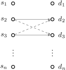
Figure 1: Illustration of selecting a $2$-element active S–D set. Here, only the second and third S–D pairs are active, while the others are silent.

Consider the following genie-aided scheme, which performs an exhaustive search over all $\binom{n}{m}$ possible ways of grouping $m$ S–D pairs, and labels the set as valid if all $m$ S–D transmissions in the set are successful. Let $X(m)$ be the number of valid sets. For certain value of $m$, $X(m)\geq 1$ implies that $mR_{0}$ total throughput is achievable. On the other hand, $\Pr[X(m)\geq 1]\to 0$ implies that $mR_{0}$ is not supportable in the probabilistic sense. (Note that the proof method enforces the condition that $\sum_{m^{\prime}>m}^{n}\Pr[X(m^{\prime})\geq 1]$ decreases to zero exponentially with $n$; see [24] for a systematic treatment of this probabilistic method of proof.) To proceed, write $X(m)$ as a sum of indicator functions:

$$X(m) =\sum_{\begin{subarray}{c}\mathcal{S}\subset\{1,\ldots,n\}\\ \lvert\mathcal{S}\rvert=m\end{subarray}}\mathbf{1}\Bigl{(}\mathsf{SINR}_{i}\geq\beta_{0},\;\forall i\in\mathcal{S}\Bigr{)}$$ (4)

$$=\sum_{\begin{subarray}{c}\mathcal{S}\subset\{1,\ldots,n\}\\ \lvert\mathcal{S}\rvert=m\end{subarray}}\mathbf{1}\Biggl{(}\frac{\gamma_{i,i}}{\frac{1}{\rho}+\sum_{\begin{subarray}{c}j\neq i\\ j\in\mathcal{S}\end{subarray}}\gamma_{j,i}}\geq\beta_{0},\;\forall i\in\mathcal{S}\Biggr{)},$$ (5)

where $\beta_{0}$ is, as before, the SINR threshold, $\rho\triangleq P/\sigma_{N}^{2}$ denotes the average SNR of the S–D link. Then, using Markov’s inequality, $\Pr[X(m)\geq 1]$ can be upper-bounded as follows:

$$\Pr[X(m)\geq 1]$$ (7)

$$\leq\mathbb{E}[X(m)]$$

$$=\binom{n}{m}\Biggl{(}\Pr\biggl{[}\frac{\gamma_{i,i}}{\frac{1}{\rho}+\sum_{\begin{subarray}{c}j\neq i\\ j\in\mathcal{S}\end{subarray}}\gamma_{j,i}}\geq\beta_{0}\biggr{]}\Biggr{)}^{m},$$

where (7) follows from the linearity of the expectation, and the fact that in our i.i.d. channel model, different $\mathsf{SINR}_{i}$s involve independent channel gains, and thus the terms $\mathsf{SINR}_{i}$s are i.i.d. over $i\in\mathcal{S}$.

The approach to find the largest $m$ for which communication is successful is to find an expression of the upper bound that is a function of $m,$ and subsequently study its behavior as a function of $m$. As detailed in the Appendix A, as far as scaling law is concerned, $\Pr\Bigl{[}\frac{\gamma_{i,i}}{\frac{1}{\rho}+\sum_{j\neq i,\,j\in\mathcal{S}}\gamma_{j,i}}\geq\beta_{0}\Bigr{]}$ is upper-bounded by $O(1/m^{2})$. In the sequel, without loss of optimality, we write $\Pr\Bigl{[}\frac{\gamma_{i,i}}{\frac{1}{\rho}+\sum_{j\neq i,\,j\in\mathcal{S}}\gamma_{j,i}}\geq\beta_{0}\Bigr{]}\leq c_{1}/m^{2}$ for some constant $c_{1}$. Then, it follows from (7) that

$$\Pr[X(m)\geq 1] \leq\binom{n}{m}\Bigl{(}\frac{c_{1}}{m^{2}}\Bigr{)}^{m}$$

$$\leq\Bigl{(}\frac{n\cdot e}{m}\Bigr{)}^{m}\Bigl{(}\frac{c_{1}}{m^{2}}\Bigr{)}^{m}$$ (8)

$$=e^{m(\log(c_{1}e\cdot n)-3\log m)},$$ (9)

where (8) follows from the inequality $\binom{n}{k}\leq(\frac{ne}{k})^{k}$.

On setting $m=(1+\varepsilon)(c_{1}e)^{1/3}\,\,n^{1/3},$ we have for any $\varepsilon>0$,

$$\Pr[X(m)\geq 1] \leq e^{-3(1+\varepsilon)\log(1+\varepsilon)(c_{1}e)^{1/3}\,n^{1/3}}$$ (10)

$$\rightarrow 0\qquad\text{as $n\rightarrow\infty$},$$ (11)

which implies that, with probability approaching $1$, we cannot find a valid set with $m=(1+\varepsilon)(c_{1}e)^{1/3}\,\cdot\,n^{1/3}$ S–D pairs. In the terminology of throughput scaling laws, the system throughput is upper-bounded by $O(n^{1/3})$.

Throughput Upper Bound of Two-hop Schemes: Next, we consider two-hop schemes, in which communication from sources to their destinations takes place in two-hop fashion, with the help of $m$ relay nodes, as illustrated in Fig. 2.

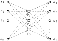
Figure 2: Illustration of a two-hop scheme with $m=3$ relay nodes. Sources $\{1,2,n\}$ form a $3$-element active source set in the first hop. Destinations $\{1,2,n\}$ form a $3$-element active destination set in the second hop.

In the following discussion, we assume that the fixed transmission rate is greater than or equal to $1$ bit/s/Hz (i.e., $R_{0}\geq 1$), and thus SINR $\geq 1$ is required at the receiver for successful communication. This additional assumption rules out the possibility that multiple transmitters can be successfully decoded by the same receiver. Accordingly, if $m$ relay nodes are deployed, the maximum number of concurrent successful transmissions is at most $m$.

We start with the first hop. Two-hop schemes differ from single-hop schemes in that they have more freedom in associating transmitter-receiver pairs. For example, in a two-hop scheme, each source can be decoded by any relay, since any relay can subsequently send the message to the intended destination. This is in contrast to single-hop schemes, in which a source must be decoded by the destined destination node. When $m$ sources are scheduled to transmit to $m$ relays, there are $m!$ ways of associating the source-to-relay (S–R) pairs. Thus, if we define $X(m)$ as the number of valid sets of $m$ concurrent S–R transmissions, we have (cf. (7))

$$\Pr[X(m)\geq 1]\leq\binom{n}{m}\,m!\,\bigl{(}\Pr[\mathsf{SINR}\geq\beta_{0}]\bigr{)}^{m}.$$

In words, to test whether $m$ concurrent S–R transmissions are possible (or equivalently if a throughput of $mR_{0}$ is achievable), a genie can search over all $\binom{n}{m}$ ways of selecting $m$-element sets of sources. Moreover, for each selection of an $m$-element set, one has $m!$ ways of associating the sources to the relays. Then, we have a total of $\binom{n}{m}\,m!$ ways of determining S–R pairs. Similar to the single-hop case, the probability of all $m$ transmissions being successful is given by $(\Pr[\mathsf{SINR}\geq\beta_{0}])^{m}$.

Analogous to (8) and (9), we have

$$\Pr[X(m)\geq 1] \leq\binom{n}{m}m!\Bigl{(}\frac{c_{1}}{m^{2}}\Bigr{)}^{m}$$

$$=\frac{n!}{(n-m)!}\Bigl{(}\frac{c_{1}}{m^{2}}\Bigr{)}^{m}$$

$$\leq\Bigl{(}c_{1}\frac{n}{m^{2}}\Bigr{)}^{m}$$

$$=e^{m(\log n-2\log m+\log c_{1})}.$$

On setting $m=(1+\varepsilon)c_{1}^{1/2}n^{1/2}$, it is straightforward to show that $\Pr[X(m)\geq 1]\rightarrow 0$. This implies that, with probability approaching $1$, one cannot have $(1+\varepsilon)c_{1}^{1/2}n^{1/2}$ concurrent successful transmissions. Equivalently, the system throughput is upper-bounded by $(1+\varepsilon)c_{1}^{1/2}n^{1/2}$. In terms of scaling laws, the throughput is $O(n^{1/2})$. Compared to the single-hop setup, we see that the additional freedom of associating transmitter–receiver pairs leads to a higher upper bound on the throughput.

According to the scheduling policy of the genie scheme, the second hop is similar to the first hop. Specifically, in the second hop, we seek among all $\binom{n}{m}\,m!$ possible ways of relaying the information from the relays to the destinations (R–D), the mappings such that all involved transmissions are successful. This is mathematically equivalent to the first hop, and therefore it results in the same upper bound on the throughput.

Combining the first hop and the second hop, we conclude that the throughput of two-hop schemes as a whole is $O(n^{1/2})$.

Throughput Upper Bound of Multihop Schemes: In multihop schemes, the communication between sources and destinations is facilitated by multiple layers of relaying.

We have discussed previously that a single layer of relays is beneficial in that it offers flexibility in routing messages between sources and destinations. However, in the random connection model stipulated in this work, there is no advantage in having multiple layers of relays. This is because in a multihop scheme, the throughput is limited by the layer with minimal throughput. Adding more relay layers does not resolve this bottleneck, and it offers no additional flexibility compared to the two-hop scheme. Therefore, as far as throughput is concerned, multihop schemes cannot do better than two-hop schemes.

This completes the proof of Theorem 1.
∎

Several remarks are in order.

Remark 1

The theorem establishes a universal upper bound on the throughput that is valid for a class of fading distributions with finite mean and variance. This class encompasses a number of familiar models in wireless communications, e.g., Rayleigh, lognormal, and Nakagami, among others. Perhaps surprisingly, particular channel model with finite mean and variance may yield the throughput scaling behavior drastically different than the upper bound of Theorem 1. For instance, it is shown in [18] that for a Rayleigh fading environment, the throughput scales as $\Theta(\log n)$, which is clearly recognized to grow much slower than $O(n^{1/2})$. Thus, in general, the throughput scaling upper bound for specific distributions should be studied on a case-by-case basis. Fortunately, for achievable throughput, insights of the throughput scaling behavior can be gained. See Remark 4 for discussion.

Remark 2

It is important to note that the conclusion that multihop schemes are not beneficial stems directly from the dense network and random fading model adopted in our work. (A similar conclusion is drawn also in [11].) In other different setups, however, multihop schemes might be beneficial. For example, in an extended network with path-loss attenuation, multiple hopping is necessary due to the limited transmission range of each hop. As a matter of fact, the nearest neighbor multihop is order-optimal in achieving the best throughput scaling in the geometrical path-loss attenuation model with attenuation factor $\alpha\geq 3$ [10].

IV Achievability of $\Theta(n^{1/2})$ Throughput

In the preceding section, we established the throughput upper bounds for different communication protocols by finding such $m$ that $\Pr[X(m)\geq 1]\rightarrow 0$. We have proved that, in the random connection channel model, two-hop schemes have a higher throughput upper bound than single-hop schemes. However, it is not clear from the preceding discussion whether this upper bound is achievable. By achievable, we mean that the scheme can operate with distributed scheduling, i.e., without the genie’s clairvoyance. In this section, we establish the achievability result of $\Theta(n^{1/2})$ for two-hop relaying schemes by a constructive example.

We formulate the achievability result in the following theorem:

Theorem 2

Under the same assumptions as Theorem 1, an average throughput scaling of $\Theta(n^{1/2})$ is achievable by a two-hop scheme.

This achievability result is established by the two-hop opportunistic relaying scheme [18]. In [18], the scheme has been shown to achieve $\Theta(\log n)$ throughput scaling under the Rayleigh fading model. In this section, we will see that the opportunistic relaying scheme is able to achieve $\Theta(n^{1/2})$ throughput scaling under the specific fading model of (1). Before proceeding to present the proof of Theorem 2, we need first to set the stage by briefly reviewing the two-hop opportunistic relaying scheme and by outlining the generic throughput expressions valid for any fading distributions (whereas the derivations in [18] are tailored to the Rayleigh fading model). Subsequently, we introduce the channel model used to prove the achievability result, and finally complete the proof.

IV-A Two-Hop Opportunistic Relaying Scheme

The two-hop opportunistic relaying scheme was first proposed in [18]. The key idea is to exploit the multiuser diversity of the network and apply it to compensate for the effect of concurrent interference sources. To enable the channel-dependent scheduling, low rate feedback is required from receivers to transmitters. For the sake of completeness, the scheduling policy of the scheme and the corresponding throughput expressions are briefly reviewed in the sequel. See [18] for details.

IV-A1 System Model

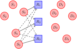
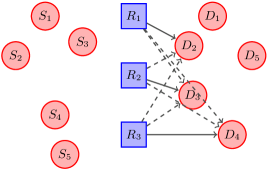
Figure 3: A two-hop network with $n=5$ S–D pairs and $m=3$ relay nodes (denoted by the blue squares). (a) In the first hop, source nodes $\{3,4,5\}$ transmit to the relays. (b) In the second hop, the relays transmit to the destination nodes $\{2,3,4\}$. Solid lines indicate scheduled links, while dashed lines indicate interference.

As illustrated in Fig. 3, we consider a wireless network with $n$ S–D pairs and $m$ relay nodes operating in a two-hop decode-and-forward fashion. Since we are interested in an achievable result, without loss of generality, we further assume a fixed transmission rate $R_{0}=1$ bit/s/Hz.

IV-A2 Scheduling and Throughput

First Hop Scheduling and Throughput: The first hop scheduling can be thought of as a natural generalization of the classic multiuser diversity scheme with single receiver antenna [25] to multiple, decentralized antennas. Specifically, denote the channel connection from $i$th source $(1\leq i\leq n)$ to $j$th relay $(1\leq j\leq m)$ as $\gamma_{i,j}$, then relay $j$ schedules its best source $i^{\ast}=\arg\max_{i}\gamma_{i,j},$ by feeding back the index $i^{\ast}$. Since there are $m$ relays, and each of them schedules one source for transmission, so up to $m$ sources can be scheduled at the same time. By accounting only for the scenario when $m$ distinct sources are scheduled (denoting such event as $N_{m}$ with $\Pr[N_{m}]=n(n-1)\cdots(n-m+1)/n^{m}$ [18]), a lower bound on throughput of the first hop $R_{1}$ can be written as,

$$R_{1} \geq\Pr[N_{m}]\sum_{j=1}^{m}\Pr[\mathsf{SINR}_{i^{\ast}\!\!,j}\geq 1]\cdot 1$$ (12)

$$=c_{2}\sum_{j=1}^{m}\Pr[\mathsf{SINR}_{i^{\ast}\!\!,j}\geq 1]\quad\text{ for some $0<c_{2}\leq 1$}$$ (13)

$$=c_{2}\,m\cdot\Pr\biggl{[}\frac{\gamma_{i^{\ast}\!\!,j}}{\frac{1}{\rho}+\sum_{\begin{subarray}{c}i\neq i^{\ast}\\ i\in\mathcal{S}\end{subarray}}\gamma_{i,j}}\geq 1\biggr{]},$$ (14)

where where right-hand side (RHS) of (12) is due to the fact that, conditioned on $N_{m}$, there are total $m$ concurrent transmissions, each transmitting $1$ bit/s/Hz with a probability of success of $\Pr[\mathsf{SINR}\geq 1]$; (13) follows from the fact that $\Pr[N_{m}]=\Theta(1)$ with $m=O(n^{1/2})$; and (14) follows from the fact that $\mathsf{SINR}_{i^{\ast}\!\!,j}$s for different $j$’s involve i.i.d. channel realizations, and thus are i.i.d. To see $\Pr[N_{m}]=\Theta(1)$ as $m=O(n^{1/2})$, we can show that the lower bound on $\Pr[N_{m}]$ is $\Theta(1)$ as follows:

$$\Pr[N_{m}] =\frac{n}{n}\frac{n-1}{n}\cdots\frac{n-m+1}{n}$$

$$\geq\left(\frac{n-m+1}{n}\right)^{m}$$

$$\geq\left(1-\frac{c_{3}\sqrt{n}-1}{n}\right)^{c_{3}\sqrt{n}}$$

with $$m=c_{3}\sqrt{n} c_{3}$$ for some constant

$$\to e^{-c_{3}^{2}}$$ (15)

$$=\Theta(1),$$

where (15) follows from the fact that $(1-x)^{n}\to e^{-nx}$ for $x\to 0$ and $n\to\infty$. Since $\Pr[N_{m}]\leq 1$, without loss of generality, we denote $\Pr[N_{m}]$ by a constant $0<c_{2}\leq 1$ in (13).

Second Hop Scheduling and Throughput: In the second hop, $m$ relay nodes communicate with destination nodes. The scheduling of the second hop works as follows. Each destination node $j$ computes $m$ SINRs (cf. (3)) by assuming that relay $k$ ($1\leq k\leq m$) is the desired sender, and all other $(m-1)$ relays generate interference. If the destination node $j$ captures one good SINR, say $\mathsf{SINR}_{k^{\ast},j}\geq 1$ for some $k^{\ast}$, it instructs relay $k^{\ast}$ to send data by feeding back the relay index $k^{\ast}$. Otherwise, the node $j$ does not provide feedback. Since the scheduling of the second hop depends on $\mathsf{SINR}\geq 1,$ by definition, all transmissions at $1$ bit/s/Hz will be successful. Consequently, the average throughput of the second hop depends on whether relay nodes are scheduled (by a destination node that measured SINR $\geq 1)$. Given the scheduling criteria as above, we have the throughput of the second hop $R_{2}$ expressed as follows

$$R_{2} =\sum_{k=1}^{m}\Pr[\text{relay $k$ is scheduled}]$$

$$=m\Pr[\text{relay $k$ is scheduled}]$$ (16)

$$=m\Pr\bigl{[}\cup_{j=1}^{n}\text{relay $k$ receives feedback from $j$}\bigr{]}$$

$$\geq m\Pr[\text{relay $k$ receives feedback from $j^{\ast}$}]$$ (17)

$$=m\cdot\Pr\biggl{[}\frac{\gamma_{k,j^{\ast}}}{\frac{1}{\rho}+\sum_{\begin{subarray}{c}k^{\prime}\neq k\\ 1\leq k^{\prime}\leq m\end{subarray}}\gamma_{k^{\prime}\!,j^{\ast}}}\geq 1\biggr{]},$$ (18)

where, again, (16) follows from our i.i.d. model and the lower bound of (17) follows from the fact we account for the event only when the best node, i.e., $j^{\ast}\triangleq\arg\max_{j}\gamma_{k,j}$, requests transmission.

Remark 3

It is noted that the scheduled policies for both the first hop and the second hop are of opportunistic nature. Consequently, it is possible that the active destination nodes in a time-slot (at the second hop) are not exactly those that correspond to the active source nodes in a previous time-slot (as deliberately exemplified in Fig. 3). Hence, the relays are assumed to have the ability to buffer the data received from source nodes, such that it is available when the opportunity arises to transmit it to the intended destination nodes over the second hop of the protocol [3]. This ensures that relays always have packets destined to the nodes that are scheduled. With the help of this assumption, the throughput of the two-hop scheme is defined as $R\triangleq\frac{1}{2}\min\{R_{1},R_{2}\},$ where $1/2$ accounts for the fact that transmitters transmit only half of time.

Remark 4

It is enlightening to look at the role played by the channel model in the throughput expressions (14) and (18). The specific channel model determines the desired signal power (the numerator) as well as the interference power. However, we know from the law of large numbers that the interference term approaches its mean value, which scales linearly with the number of relays $m$. However, the signal power is more sensitive to channel models (i.e., different models have different multiuser diversity gains). For example, the multiuser diversity gain scales as $\log n$ for Rayleigh fading channels [22], but scales as $e^{\sqrt{2\log n}\,\sigma}$ for lognormal fading channels [26, Sec. 2.3.3., p. 67]. In order to have non-diminishing data rate, we need accordingly non-diminishing SINR. Therefore, the limiting operating scenario would be that the desired signal strength (i.e., the multiuser diversity gain) is of the same order as the aggregate interference power. This implies that the maximal number of scheduled transmissions (and hence the maximal throughput) is governed by the order of multiuser diversity gain. This intuition is explored numerically in [27] for various fading models.

IV-B Channel Model

Given the intuition from Remark 4, for $\Theta(n^{1/2})$ throughput scaling, a fading distribution is required that has a multiuser diversity gain of the order of $\Theta(n^{1/2})$. To this end, we assume the channel (power) gains (S–R and R–D) are drawn independently from the following cdf:

$$F_{n}(x)=\biggl{(}\frac{(x-\mu)/\sigma}{\sqrt{2n-1}}\frac{n-1}{n}+\frac{1}{n}\biggr{)}^{1/(n-1)},$$ (19)

$$\mu-\tfrac{\sqrt{2n-1}}{n-1}\sigma\leq x\leq\mu+\sqrt{2n-1}\sigma,$$

where $\mu$ and $\sigma$ are respectively, the mean and variance of the fading connection, and are assumed to be finite.

Indeed, the cdf in (19) has the unique property that it maximizes the expectation of the extreme value among all distributions possessing finite mean and variance [28]. Moreover, the mean is given by $\mathbb{E}[M_{n}]=\mu+\sigma\frac{n-1}{\sqrt{2n-1}}$, where $M_{n}$ denotes the maximum of $n$ i.i.d. random variables having the common distribution of (19).

In what follows, we assume $\mu=\sigma=1$. This simplification incurs no loss of optimality with respect to the scaling behavior. The following property, easily verified (see Appendix B for derivation), will be useful in the ensuing discussion:

$$\Pr\left[M_{n}>\frac{n-1}{\sqrt{2n-1}}\right]=\Pr\left[M_{n}\leq\frac{n-1}{\sqrt{2n-1}}\right]=\frac{1}{2}.$$ (20)

$$\Pr [\mathsf{SINR}\geq 1]\approx\Pr\biggl{[}\frac{M_{n}}{I_{m-1}}\geq 1\biggr{]}$$ (23)

$$=\underbrace{\Pr\biggl{[}\frac{M_{n}}{I_{m-1}}\geq 1\bigg{|}M_{n}>m,I_{m-1}\leq m\biggr{]}}_{=1}\Pr[M_{n}>m,I_{m-1}\leq m]$$

$$\quad+\underbrace{\Pr\biggl{[}\frac{M_{n}}{I_{m-1}}\geq 1\bigg{|}M_{n}>m,I_{m-1}>m\biggr{]}}_{\geq 0}\Pr[M_{n}>m,I_{m-1}>m]$$

$$\quad+\underbrace{\Pr\biggl{[}\frac{M_{n}}{I_{m-1}}\geq 1\bigg{|}M_{n}\leq m,I_{m-1}\leq m\biggr{]}}_{\geq 0}\Pr[M_{n}\leq m,I_{m-1}\leq m]$$

$$\quad+\underbrace{\Pr\biggl{[}\frac{M_{n}}{I_{m-1}}\geq 1\bigg{|}M_{n}\leq m,I_{m-1}>m\biggr{]}}_{=0}\Pr[M_{n}\leq m,I_{m-1}>m]$$

$$\geq\Pr[M_{n}>m,I_{m-1}\leq m]$$ (24)

$$\geq\frac{1}{26},$$ (25)

IV-C Proof of Achievability

Before embarking on the achievability proof, we first characterize the aggregate interference stemming from all $(m-1)$ concurrent transmitting sources, $\sum_{i\neq i^{\ast},\,i\in\mathcal{S}}\gamma_{i,j}$, in the expressions of (14) and (18). It is shown in [18] that, in the regime of large $n$, the $\{\gamma_{i,j}\}$ are asymptotically independent. Denote $I_{m-1}\triangleq\sum_{i\neq i^{\ast},\,i\in\mathcal{S}}\gamma_{i,j}$. In the ensuing achievability proof, we need to show that $\Pr[I_{m-1}\leq m]$ is at least greater than zero. To show this, we need the following technical lemma due to Feige [29, Th. 1].

Lemma 1

Let $X_{1},\ldots,X_{N}$ be arbitrary nonnegative independent random variables, with expectations $\mathbb{E}[X_{i}]\leq 1,\,\forall\,i$. Let $S=\sum_{i=1}^{N}X_{i}$. Then for every $\delta>0$,

$$\Pr\bigl{[}S\leq\mathbb{E}[S]+\delta\bigr{]}\geq\min\left(\frac{\delta}{1+\delta},\frac{1}{13}\right).$$ (21)

In our case, from the linearity of expectation, we have $\mathbb{E}[I_{m-1}]=m-1$. Thus, from (21) we have:

$$\Pr\bigl{[}I_{m-1}\leq m\bigr{]}\geq\min\left(\frac{1}{2},\frac{1}{13}\right)=\frac{1}{13}.$$ (22)

The proof of Theorem 2 follows now.

Proof:

Both lower bounds (14) and (18) manifest a tradeoff between data rate and interference: Increasing the number of relay nodes is beneficial from the rate’s perspective, but the interference term is also increased. Since the operating SINR threshold is one, a good operating point for $m$ should be such that the SINR is of the order of one. Hence, noting the fact that the mean value of the signal power is given by $\mathbb{E}[M_{n}]=1+\frac{n-1}{\sqrt{2n-1}}$, we set the number of relay nodes $m$ to $\frac{n-1}{\sqrt{2n-1}}$. This specific setup causes $\Pr[\mathsf{SINR}\geq 1]$ in (14) and (18) to be of the order of one. Specifically, in the derivation, which is shown at the bottom of the page, the approximation in (23) is due to the fact that Gaussian noise is ignored (note that the system is interference limited); the inequality in (24) follows since one combination of $M_{n}$ and $I_{m-1}$ is accounted for in applying the total probability theorem; and (25) follows from the fact that $M_{n}$ and $I_{m-1}$ are asymptotically independent [18] and from (22).

Together, $m=\frac{n-1}{\sqrt{2n-1}}$ and (25) lead to the conclusion that both (14) and (18) are greater than or equal to $\frac{1}{26}\frac{n-1}{\sqrt{2n-1}}$, which scales as $\Theta(n^{1/2})$ as $n\rightarrow\infty$. This completes the proof of Theorem 2. ∎

Remark 5

In this section, we have focused on the achievability of $\Theta(n^{1/2})$ for two-hop schemes. To this end, we have introduced the connection model of (19), which is a function of $n$. While such a distribution is not likely to be encountered in practice, the result of Theorem 2 is still of theoretical importance as it confirms that the $O(n^{1/2})$ upper bound in Theorem 1 is tight.

Finally, it is important to note that the achievability of the result in this section is established for the specific two-hop opportunistic relaying scheme. In pursuing the achievable $O(n^{1/2})$ throughput, it is of both theoretical and practical interest to study other relaying schemes and examine their achievable throughputs under other channel models.

V Beyond $\Theta(n^{1/2})$

The preceding sections restrict the discussion to a class of channel connection distributions possessing finite mean and variance. Theorems 1 and 2 state that, for such fading distributions, the throughput is upper-bounded by $\Theta(n^{1/2})$. Now, a natural question to ask is whether there exist channel models that can yield better, even linear, throughput scaling?

It turns out that the answer is affirmative. Again, since achievable results are concerned, a case study suffices. To this end, we show in this section that the two-hop opportunistic relaying scheme (cf. Section IV-A) yields linear throughput scaling under a class of fading models. This motivates in the second part of the section, a broader discussion on channel models.

V-A Linear Throughput Scaling

The key to attaining linear throughput scaling with the opportunistic scheme is to achieve non-vanishing SINR (cf. (3)) even when $n\rightarrow\infty$. Intuitively, in order to achieve $\Theta(n)$ throughput scaling, one has to schedule $\Theta(n)$ concurrent transmissions and at the same time to have $\Pr[\mathsf{SINR}\geq\beta_{0}]>0$ as $n\to\infty$. We know from the discussion in Section IV that the latter is not possible if the underlying channel model has finite mean and variance. This is because the interference increases linearly with $n,$ but the signal power grows no faster than $n^{1/2}$. Nevertheless, the following result shows that if we relax the requirement of finite mean and variance, there exists a class of fading models for which the signal power increases linearly with $n$.

Lemma 2

Let $X_{1},\ldots,X_{n}$ be independent random variables with common cdf $F$ satisfying

$$1-F(x)\sim\frac{c_{0}\cdot x^{-\nu}}{\Gamma(1-\nu)}$$ (26)

where $0<\nu<1$, $c_{0}$ is a constant, and $\Gamma(x)$ is the gamma function. Define $I_{n}=X_{1}+\cdots+X_{n}$ and $M_{n}=\max\{X_{1},\ldots,X_{n}\}$; then

$$\Pr\biggl{[}\frac{M_{n}}{I_{n}}\geq 1-\nu\biggr{]}>0$$ (27)

as $n\rightarrow\infty$.

Proof:

See Appendix C. ∎

Note that (27) holds independently of the system size. In other words, we can equivalently write $\Pr\bigl{[}\frac{M_{n}}{I_{n}}\geq 1-\nu\bigr{]}=c_{4}$ for some constant $c_{4}>0$ as $n\to\infty$. This is in contrast to the fading distributions that we have studied in Section III. There $\Pr[\mathsf{SINR}\geq\beta_{0}]$ decreases to zero as $m$ increases.

With the help of the lemma, one can set the system parameters of the two-hop opportunistic relaying scheme as follows to achieve linear throughput scaling. First, set SINR threshold $\beta_{0}=1-\nu$, and the corresponding $R_{0}=\log(2-\nu)$. Then, set $m=n$ (i.e., deploy as many relay nodes as S–D pairs). Under this setup, it is then straightforward to show that the total number of scheduled transmissions is of the order of $n$, i.e., $\mathbb{E}[\lvert\mathcal{S}\rvert]=\Theta(n)$ (see Appendix D for the derivation). This fact, together with the fact that each of S–D pairs has a successful transmission probability greater than zero (cf. (27)), means that the system has linear throughput scaling. We summarize this result in the following theorem:

Theorem 3

A linear average throughput scaling of $\Theta(n)$ is achievable by the two-hop relaying scheme under fading models satisfying (26).

Example 1

To show the application of Theorem 3, it is illuminating to revisit the famous Grossglauser–Tse scheme [3], but under the framework of the random connection model.

In [3], the authors considered a network model in which all nodes are assumed to move in an i.i.d., stationary, and ergodic fashion over a fixed area. The channel connections between nodes are determined by a path-loss attenuation model, i.e., the connection between any two nodes follows a path-loss law $g(r)=\sqrt{G}\frac{1}{r^{\alpha}},$ where $r$ is the distance between the nodes, $\alpha\geq 2$ is the path-loss exponent, and $G$ is a constant depending on system parameters. It is shown that a two-hop relaying scheme featuring nearest-neighbor communication can achieve a linear throughput scaling. Note that the geometric path-loss attenuation model used in [3] can be thought of as a particular random fading model, where the randomness stems from the random distance between nodes. For example, for each transmitter, the received power seen by all receiving nodes are random since distances are random. Following the approach of [11, Sec. VIII.B], one can in fact characterize the distribution of the received powers as follows. Consider a simplified scenario where a source node at the center of a unit area. All receiver nodes are assumed to be uniformly distributed over the area. The node has transmit power $P$ and we denote $\gamma$ the corresponding received power. Now, for a typical receiver, the probability of receiving power less than $\gamma P$ is given by

$$F(\gamma)=1-\pi\gamma^{-\frac{2}{\alpha}}$$ (28)

where $\gamma\in[\pi^{\frac{\alpha}{2}},\infty]$. Now, we can interpret the original Grossglauser–Tse scheme as though it is in the framework of the random connection model with fading distribution specified by (28). Seen another way, if we allow mobility of nodes in a network with path-loss attenuation model, mobility effectively blurs the distinction between near and far nodes and the network exhibits homogeneity. From the effective channel connection’s perspective, the network is equivalent to operating under random channel model (28). Consequently, the linear throughput achievability of [3] can be explained by noting the fact that the distribution of (28) is of the form of (26) (with $\nu=2/\alpha$ and $c_{0}=\pi\,\Gamma(1-2/\nu)$). As a matter of fact, the distribution of (28) is referred to as a Pareto distribution [30]. The Pareto distribution is known to have infinite mean, when $2/\alpha\leq 1,$ and infinite variance when $2/\alpha\leq 2$. This is consistent with Theorem 1.

It is important to point out that, though linear throughput scaling is achievable, it does not mean that the system performance is not hindered by interference. The effect of interference is revealed in that increasing the transmission power of each node does not lead to an increase in throughput. What happens is that, thanks to the unique property of the Pareto distribution, we can operate at the boundary between interference-limited and degrees of freedom-limited regimes.

As a final remark, it should be noted that Theorem 3 provides just one type of channel models that can yield linear throughput scaling, and it does not preclude the existence of other distributions that can yield linear throughput scaling.

V-B Discussion On The Channel Model

Unlike [1, 3, 5, 10] (among many others) in which geometric path-loss channel models are assumed, this paper adopts the random connection model initially proposed in [11]. In the random connection model, there is no notion of location and distance. Instead, the channel connections are modeled as random variables. This model applies to scenarios where the network is physically small such that path-loss is less relevant or where the mechanism of automatic gain control (AGC) is used to mitigate path-loss attenuation. This former scenario is partially justified by the channel measurements in [32]. There, the authors report that, in vehicle-to-vehicle communication environment, the standard deviation of channel strength can be as large as $17.5$ dB.

On the other hand, when large-scale path-loss attenuation becomes significant, the recent work [33] formulated the network in terms of three system parameters: short-distance SNR (defined as the SNR over the typical nearest neighbor distance), long-distance SNR (defined as the SNR over the largest scale in the network), and the power path-loss exponent. Depending on various combinations of the values of these parameters, four fundamental operating regimes of wireless networks have been identified. One interesting regime is when the network is heterogeneous in nature, namely, the short-distance SNR is large but the long-distance SNR is small. It turns out that optimal scheme in this regime follows the principle of “cooperate locally but multihop globally,” that is, the optimal scheme should cooperate locally within clusters of intermediate size and then multihop across clusters to reach the destination. Focusing on the communication within the cluster, we note that the random connection model of this work is a natural candidate.

VI Concluding Remarks

This work has focused on the throughput scaling laws of fading networks in the limit of a large number of nodes. Motivated by considerations of CSI availability, we have considered the case in which receivers have perfect CSI, but transmitters have only partial CSI via receiver feedback. We have characterized the architectural differences between various communication protocols from the throughput standpoint. Specifically, it has been shown that for a class of fading channels with finite mean and variance, the upper bound on the throughput scaling is given by $O(n^{1/3})$ for single-hop schemes, and by $O(n^{1/2})$ for two-hop (and multihop) schemes. We have also shown that the two-hop opportunistic relaying scheme achieves the $\Theta(n^{1/2})$ throughput scaling upper bound. Furthermore, by relaxing the constraints of finite mean and variance of the fading model, we have shown that linear throughput scaling $\Theta(n)$ is achievable with Pareto-type fading models with the two-hop opportunistic relaying scheme.

Some interesting issues remain open. First, are there other relaying schemes which achieve the $O(n^{1/2})$ throughput under more realistic channel models? Another important question that is not addressed in this paper is whether the $O(n^{1/3})$ throughput upper bound for a single-hop scheme is achievable or not. It is also interesting to characterize what happens if we alleviate the assumption of conventional single-user decoding at the receivers (e.g., allowing interference cancelation and joint decoding techniques), but keep the CSI availability framework. Finally, while this work assumes dedicated relays (which have no intrinsic traffic demands), it is of interest to look at the ad hoc setup in which a dynamic subset of nodes (source and destination) act as relays.

Appendix A Derivation of the Upper Bound of $\Pr\Bigl{[}\frac{\gamma_{i,i}}{\frac{1}{\rho}+\sum_{j\neq i,\,j\in\mathcal{S}}\gamma_{j,i}}\geq\beta_{0}\Bigr{]}$

In this appendix, the upper bound on $\Pr\Bigl{[}\frac{\gamma_{i,i}}{\frac{1}{\rho}+\sum_{j\neq i,\,j\in\mathcal{S}}\gamma_{j,i}}\geq\beta_{0}\Bigr{]}$ is derived in the asymptotic regime of large $m$. For notational convenience, let $Z\triangleq\sum_{\begin{subarray}{c}j\neq i\\ j\in\mathcal{S}\end{subarray}}\gamma_{j,i}$. Starting with the law of total probability, for any $s>0$, we have

$$\Pr\left[\frac{\gamma_{i,i}}{1/\rho+Z}\geq\beta_{0}\right]$$ (31)

$$=\Pr\left[\frac{\gamma_{i,i}}{1/\rho+Z}\geq\beta_{0}\biggl{|}Z\leq s\right]\Pr[Z\leq s]$$

$$\quad+\Pr\left[\frac{\gamma_{i,i}}{1/\rho+Z}\geq\beta_{0}\biggl{|}Z>s\right]\Pr[Z>s]$$

$$\leq\Pr[Z\leq s]+\Pr\left[\frac{\gamma_{i,i}}{1/\rho+Z}\geq\beta_{0}\biggl{|}Z>s\right]$$

$$\leq\Pr[Z\leq s]+\Pr\left[\frac{\gamma_{i,i}}{1/\rho+s}\geq\beta_{0}\right],$$

where (31) follows from the fact that $\Pr\Bigl{[}\frac{\gamma_{i,i}}{1/\rho+Z}\geq\beta_{0}\bigl{|}Z\leq s\Bigr{]}\leq 1$ and $\Pr[Z>s]\leq 1$. Now, we proceed to upper-bound each term in (31).

To bound $\Pr[Z\leq s]$, we need the following large deviation result due to Maurer [34, Th. 2.1].

Theorem 4

Let $X_{1},\ldots,X_{N}$ be independent real-valued random variables with $X_{i}\geq 0$ and $\mathbb{E}[X_{i}^{2}]<\infty$ for $i=1,\ldots,N$. Set $S=\sum_{i=1}^{N}X_{i}$ and let $x>0$. Then

$$\Pr[S\leq\mathbb{E}[S]-Nx]\leq\exp\left(-\frac{N^{2}x^{2}}{2\sum_{i=1}^{N}\mathbb{E}[X_{i}^{2}]}\right).$$ (32)

In our case where $\gamma_{j,i}$s are i.i.d. with finite means $\mu$ and variances $\sigma^{2}$, and $Z=\sum_{\begin{subarray}{c}j\neq i\\ j\in\mathcal{S}\end{subarray}}\gamma_{j,i}$ with $\lvert\mathcal{S}\rvert=m$, we have $\mathbb{E}[Z]=(m-1)\mu$ and $\mathbb{E}[\gamma_{j,i}^{2}]=\mu^{2}+\sigma^{2}$. Then, the above inequality can be written as

$$\Pr[Z\leq(m-1)(\mu-x)]\leq\exp\left(-\frac{(m-1)x^{2}}{2(\mu^{2}+\sigma^{2})}\right).$$ (33)

Finally, in order to have the form of $\Pr[Z\leq s]$ as in (31), set $(m-1)(\mu-x)=s$ and accordingly we have

$$\Pr[Z\leq s]\leq\exp\left(-\frac{(m-1)(\mu-\frac{s}{m-1})^{2}}{2(\mu^{2}+\sigma^{2})}\right),$$ (34)

for $s<(m-1)\mu$ (due to the fact $x>0$).

Next, we upper-bound $\Pr\bigl{[}\frac{\gamma_{i,i}}{1/\rho+s}\geq\beta_{0}\bigr{]}$:

$$\Pr\biggl{[}\frac{\gamma_{i,i}}{1/\rho+s}\geq\beta_{0}\biggr{]}$$ (36)

$$=\Pr\bigl{[}\gamma_{i,i}\geq\beta_{0}(1/\rho+s)\bigr{]}$$

$$=\Pr\bigl{[}\gamma_{i,i}-\mu\geq\beta_{0}(1/\rho+s)-\mu\bigr{]}$$

$$\leq\Pr\bigl{[}\lvert\gamma_{i,i}-\mu\rvert\geq\beta_{0}(1/\rho+s)-\mu\bigr{]}$$

$$\leq\frac{\sigma^{2}}{(\beta_{0}s+\beta_{0}/\rho-\mu)^{2}},$$

where (36) follows from the Chebyshev inequality. Note that for (36) to hold, we need $\beta_{0}(1/\rho+s)-\mu\geq 0$, i.e., $s\geq\frac{\mu}{\beta_{0}}-\frac{1}{\rho}$.

Substituting (34) and (36) into (31), with $\frac{\mu}{\beta_{0}}-\frac{1}{\rho}\leq s<(m-1)\mu$, we have

$$\begin{split}\Pr\left[\frac{\gamma_{i,i}}{1/\rho+Z}\geq\beta_{0}\right]&\leq\exp\left(-\frac{(m-1)(\mu-\frac{s}{m-1})^{2}}{2(\mu^{2}+\sigma^{2})}\right)\\ &\quad+\frac{\sigma^{2}}{(\beta_{0}s+\beta_{0}/\rho-\mu)^{2}}.\\ \end{split}$$ (37)

Note that (37) holds for all $s$ satisfying $\frac{\mu}{\beta_{0}}-\frac{1}{\rho}\leq s<(m-1)\mu$. In the problem under discussion, it suffices to set $s=\frac{m-1}{2}\mu$. Then it follows immediately that the first term on the RHS of (37) decays exponentially with $m$, while the second term decays as $\frac{1}{m^{2}}$. Thus, as far as scaling is concerned, $\Pr\Bigl{[}\frac{\gamma_{i,i}}{\frac{1}{\rho}+\sum_{j\neq i,\,j\in\mathcal{S}}\gamma_{j,i}}\geq\beta_{0}\Bigr{]}$ is upper-bounded by $O(1/m^{2})$.

Appendix B Derivation of (20)

From (19), the cdf of the extreme value $M_{n}$ can be written as follows (with the assumption of $\mu=\sigma=1$)

$$F_{M_{n}}(x)=\left(F_{n}(x)\right)^{n}=\biggl{(}\frac{x-1}{\sqrt{2n-1}}\frac{n-1}{n}+\frac{1}{n}\biggr{)}^{n/(n-1)}.$$ (38)

It can be easily verified that $\lim_{n\rightarrow\infty}$ $F_{M_{n}}(\mathbb{E}[M_{n}])=1/2$. For increasing $n,$ we have $\mathbb{E}\left[M_{n}\right]\approx\frac{n-1}{\sqrt{2n-1}}$; it follows that

$$\Pr\biggl{[}M_{n}>\frac{n-1}{\sqrt{2n-1}}\biggr{]}=\Pr\biggl{[}M_{n}\leq\frac{n-1}{\sqrt{2n-1}}\biggr{]}=\frac{1}{2}.$$

Appendix C Proof of Lemma 2

We start by quoting the following results from [30, Problem 26, pp. 465]. (The proof follows readily from the hint for the solution, and therefore it is omitted here.) If the distribution satisfies the conditions of Lemma 2, it is known that:

1. The distribution of the ratio $I_{n}/M_{n}$ has a Laplace transform $w_{n}(\lambda)$ converging to $w(\lambda)=\frac{e^{-\lambda}}{1+\nu\int_{0}^{1}(1-e^{-\lambda t})t^{-\nu-1}\mathrm{d}t}$;

2. $\mathbb{E}[I_{n}/M_{n}]\rightarrow 1/(1-\nu)$.

Now, we can proceed with proving $\Pr[{M_{n}}/{I_{n}}\geq 1-\nu]>0$ by contradiction. Suppose $\Pr[{M_{n}}/{I_{n}}\geq 1-\nu]=0$, then

$$\mathbb{E}[M_{n}/I_{n}] =\int_{0}^{\infty}(1-F(x))\,\mathrm{d}x$$ (39)

$$=\int_{0}^{\infty}\Pr[{M_{n}}/{I_{n}}\geq x]\,\mathrm{d}x$$ (40)

$$=\int_{0}^{1-\nu}\Pr[{M_{n}}/{I_{n}}\geq x]\,\mathrm{d}x$$

$$\quad+\underbrace{\int_{1-\nu}^{\infty}\Pr[{M_{n}}/{I_{n}}\geq x]\,\mathrm{d}x}_{=0}$$ (41)

$$\leq 1-\nu,$$ (42)

where (39) follows from the fact that $\mathbb{E}[X]=\int_{0}^{\infty}(1-F(x))\mathrm{d}x$ for continuous and nonnegative random variables.

However, by Jensen’s inequality, we have $\mathbb{E}[M_{n}/I_{n}]\geq 1/\mathbb{E}[I_{n}/M_{n}]=1-\nu$. Therefore, we have $\mathbb{E}[M_{n}/I_{n}]=1-\nu$, implying that equality holds in Jensen’s inequality. This is only when the distribution of the random variable $I_{n}/M_{n}$ is degenerate (i.e., $I_{n}/M_{n}$ is a constant). However, this contradicts property $1$) which implies a non-degenerate distribution.

Thus, $\Pr[{M_{n}}/{I_{n}}\geq 1-\nu]>0$ must hold.

Appendix D Average Number of Scheduled Transmissions is $\Theta(n)$

Under the setting of $m=n$ (i.e., deploying as many relay nodes as S–D pairs), it is shown that the average number of scheduled concurrent transmissions in the two-hop opportunistic relaying scheme is of the order of $n$. To see this, define

$$Z_{i}=\begin{cases}1,&\text{if receiver $i$ is scheduled,}\\ 0,&\text{otherwise,}\end{cases}$$

so that the number of scheduled sources is written as

$$Z=Z_{1}+\cdots+Z_{n}.$$

Linearity of the expectation yields,

$$\mathbb{E}[Z]=\mathbb{E}[Z_{1}]+\cdots+\mathbb{E}[Z_{n}].$$

For each $i$, $Z_{i}$ has a simple Bernoulli distribution. Specifically, in the i.i.d. random model of Section II, each source has probability of $1/n$ to be selected by any relay. We have

$$\mathbb{E}[Z_{i}] =\Pr[\text{node $i$ is scheduled}]$$

$$=1-\Pr[\text{node $i$ is not scheduled}]$$

$$=1-\biggl{(}1-\frac{1}{n}\biggr{)}^{n}$$

$$\rightarrow 1-e^{-1},$$

where the last equation follows from the fact $(1-x)^{n}\rightarrow e^{-nx}$ for $x\rightarrow 0$. Finally, we readily have

$$\mathbb{E}[Z]=n(1-e^{-1}),$$ (43)

which is $\Theta(n)$.

References

- [1] P. Gupta and P. R. Kumar, “The capacity of wireless networks,” IEEE Trans. Inf. Theory, vol. 46, no. 2, pp. 388–404, Mar. 2000.
- [2] M. Franceschetti, O. Dousse, D. N. C. Tse, and P. Thiran, “Closing the gap in the capacity of wireless networks via percolation theory,” IEEE Trans. Inf. Theory, vol. 53, no. 3, pp. 1009–1018, Mar. 2007.
- [3] M. Grossglauser and D. N. C. Tse, “Mobility increases the capacity of ad hoc wireless networks,” IEEE/ACM Trans. Netw., vol. 10, no. 4, pp. 477–486, Aug. 2002.
- [4] S. N. Diggavi, M. Grossglauser, and D. N. C. Tse, “Even one-dimensional mobility increases the capacity of wireless networks,” IEEE Trans. Inf. Theory, vol. 51, no. 11, pp. 3947–3954, Nov. 2005.
- [5] L.-L. Xie and P. R. Kumar, “A network information theory for wireless communication: Scaling laws and optimal operation,” IEEE Trans. Inf. Theory, vol. 50, no. 5, pp. 748–767, May 2004.
- [6] ——, “On the path-loss attenuation regime for positive cost and linear scaling of transport capacity in wireless networks,” IEEE Trans. Inf. Theory, vol. 52, no. 6, pp. 2313–2328, Jun. 2006.
- [7] A. Jovičić, P. Viswanath, and S. R. Kulkarni, “Upper bounds to transport capacity of wireless networks,” IEEE Trans. Inf. Theory, vol. 50, no. 11, pp. 2555–2565, Nov. 2004.
- [8] F. Xue, L.-L. Xie, and P. R. Kumar, “The transport capacity of wireless networks over fading channels,” IEEE Trans. Inf. Theory, vol. 51, no. 3, pp. 834–847, Mar. 2005.
- [9] O. Lévêque and İ. E. Telatar, “Information-theoretic upper bounds on the capacity of large extended ad hoc wireless networks,” IEEE Trans. Inf. Theory, vol. 51, no. 3, pp. 858–865, Mar. 2005.
- [10] A. Özgür, O. Lévêque, and D. N. C. Tse, “Hierarchical cooperation achieves optimal capacity scaling in ad hoc networks,” IEEE Trans. Inf. Theory, vol. 53, no. 10, pp. 3549–3572, Oct. 2007.
- [11] R. Gowaikar, B. M. Hochwald, and B. Hassibi, “Communication over a wireless network with random connections,” IEEE Trans. Inf. Theory, vol. 52, no. 7, pp. 2857–2871, Jul. 2006.
- [12] S. Aeron and V. Saligrama, “Wireless ad hoc networks: Strategies and scaling laws for the fixed SNR regime,” IEEE Trans. Inf. Theory, vol. 53, no. 6, pp. 2044–2059, Jun. 2007.
- [13] A. Høst-Madsen and A. Nosratinia, “The multiplexing gain of wireless networks,” in Proc. IEEE Int. Symp. Information Theory, Adelaide, Australia, Sep. 2005.
- [14] V. R. Cadambe and S. A. Jafar, “Interference alignment and degrees of freedom of the –user interference channel,” IEEE Trans. Inf. Theory, vol. 54, no. 8, pp. 3425–3441, Aug. 2008.
- [15] A. F. Dana and B. Hassibi, “On the power efficiency of sensory and ad hoc wireless networks,” IEEE Trans. Inf. Theory, vol. 52, no. 7, pp. 2890–2914, Jul. 2006.
- [16] V. I. Morgenshtern and H. Bölcskei, “Crystallization in large wireless networks,” IEEE Trans. Inf. Theory, vol. 53, no. 10, pp. 3319–3349, Oct. 2007.
- [17] M. Ebrahimi, M. A. Maddah-Ali, and A. K. Khandani, “Throughput scaling laws for wireless networks with fading channels,” IEEE Trans. Inf. Theory, vol. 53, no. 11, pp. 4250–4254, Nov. 2007.
- [18] S. Cui, A. M. Haimovich, O. Somekh, and H. V. Poor, “Opportunistic relaying in wireless networks,” IEEE Trans. Inf. Theory, vol. 55, no. 11, pp. 5121–5137, Nov. 2009.
- [19] R. Etkin, “Spectrum sharing: Fundamental limits, scaling laws, and self-enforcing protocols,” Ph.D. dissertation, Univ. California, Berkeley, Dec. 2006.
- [20] G. J. Foschini, “Layered space-time architecture for wireless communication in a fading environment when using multi-element antennas,” Bell Labs. Tech. J, vol. 1, no. 2, pp. 41–59, 1996.
- [21] İ. E. Telatar, “Capacity of multi-antenna Gaussian channels,” Europ. Trans. Telecommun., vol. 10, pp. 585–595, Nov. 1999.
- [22] P. Viswanath, D. N. C. Tse, and R. Laroia, “Opportunistic beamforming using dumb antennas,” IEEE Trans. Inf. Theory, vol. 48, no. 6, pp. 1277–1294, Jun. 2002.
- [23] M. Ebrahimi, M. A. Maddah-Ali, and A. K. Khandani, “Throughput scaling in decentralized single-hop wireless networks with fading channels,” Univ. of Waterloo, Canada, Tech. Rep. UW-ECE #2006–13, 2006.
- [24] N. Alon and J. H. Spencer, The Probabilistic Method, 2nd ed. New York: Wiley, 2000.
- [25] R. Knopp and P. Humblet, “Information capacity and power control in single cell multiuser communications,” in Proc. IEEE Int. Conf. Communications, vol. 1, Seattle, WA, Jun. 1995, pp. 331–335.
- [26] J. Galambos, The Asymptotic Theory of Extreme Order Statistics, 1st ed. New York: Wiley, 1978.
- [27] S. Cui and A. M. Haimovich, “Multiuser diversity in wireless ad hoc networks,” in Proc. IEEE Global Communications Conf., New Orleans, LA, Nov.-Dec. 2008.
- [28] E. J. Gumbel, “The maxima of the mean largest value and of the range,” Ann. Math. Statist., vol. 25, pp. 76–84, Mar. 1954.
- [29] U. Feige, “On sums of independent random variables with unbounded variance, and estimating the average degree in a graph,” SIAM J. Comput., vol. 35, no. 4, pp. 964–984, 2006.
- [30] W. Feller, An Introduction to Probability Theory and Its Applications, 2nd ed. New York: Wiley, 1971, vol. II.
- [31] L. Zheng and D. N. C. Tse, “Diversity and multiplexing: a fundamental tradeoff in multiple-antenna channels,” IEEE Trans. Inf. Theory, vol. 49, no. 5, pp. 1073–1096, May 2003.
- [32] J. Ling, D. Chizhik, D. Samardzija, and R. A. Valenzuela, “Peer-to-peer MIMO radio channel measurements in a rural area,” IEEE Trans. Wireless Commun., vol. 6, no. 9, pp. 3229–3237, Sep. 2007.
- [33] A. Özgür, R. Johari, D. N. C. Tse, and O. Lévêque, “Information theoretic operating regimes of large wireless networks,” IEEE Trans. Inf. Theory, vol. 56, no. 1, pp. 427–437, Jan. 2010.
- [34] A. Maurer, “A bound on the deviation probability for sums of nonnegative random variables,” J. Inequalities Pure Appl. Math, vol. 4, no. 1, 2003, article 15.