Integral Field Spectroscopy of HH 262: The Spectral Atlas

Abstract

HH 262 is a group of emitting knots displaying an ”hour-glass” morphology in the H$\alpha$ and [S ii] lines, located 3.5 arcmin to the northeast of the young stellar object L1551-IRS5, in Taurus. We present new results of the kinematics and physical conditions of HH 262 based on Integral Field Spectroscopy covering a field of $\sim$ 1.5 $\times$ 3 arcmin², which includes all the bright knots in HH 262. These data show complex kinematics and significant variations in physical conditions over the mapped region of HH 262 on a spatial scale of $\leq$ 3 arcsec. A new result derived from the IFS data is the weakness of the [N ii] emission (below detection limit in most of the mapped region of HH 262), including the brightest central knots. Our data reinforce the association of HH 262 with the redshifted lobe of the evolved molecular outflow L1551-IRS5. The interaction of this outflow with a younger one, powered by L1551 NE, around the position of HH 262 could give rise to the complex morphology and kinematics of HH 262.

1 Introduction

HH 262 is the designation of a group of emitting knots, surrounded by more diffuse emission, located $\sim$ 3.5 arcmin to the northeast of the source L1551-IRS5 in Taurus. The two brightest HH 262 condensations (named GH9 and GH10) were first reported by Rodríguez et al. (1989) and Graham & Heyer (1990). In the H$\alpha$+[N ii] and [S ii] narrow-band images, HH 262 shows a rather chaotic, ”hour-glass”-shaped morphology that is quite different from the collimated structures found in most of the Herbig–Haro (HH) jets (Garnavich, Noriega-Crespo & Green 1992, López et al. 1995). Apparently, the morphology of HH 262 seems to trace a wind-blown cavity from an embedded source located close to the GH10 knot. However, no point source suitable for powering the HH 262 emission has been currently reported at this location. Since its discovery, the origin of HH 262, as well as its relationship with other outflows in the L1551 star-forming region, has been matter of discussion. Rodríguez et al. (1989) first suggested that the GH9 and GH10 knots were associated with the redshifted lobe of the molecular outflow powered by the source L1551-IRS5. They proposed that GH9 and GH10 may be the redshifted counterpart of a chain of HH bright knots (which includes the well-known HH objects 28 and 29) extending from L1551-IRS5 to the southwest up to $\sim$ 5 arcmin, and suggested that all these optical knots traced the walls of a wind cavity evacuated by the CO outflow powered by L1551-IRS5.

Later on, Graham & Rubin (1992) obtained a long-slit spectrum across the GH9 and GH10 knots. From the H$\alpha$ line, they derived redshifted radial velocities covering a range extending over $\sim$ 100 km s^-1and measure peak velocities of +40 km s^-1 and +90 km s^-1 and average velocities of +20 km s^-1and +45 km s^-1in the GH9 and GH10 knots, respectively. These results reinforced the suggestion that GH9 and GH10 were associated with the redshifted lobe of the CO outflow powered by L1551-IRS5. The kinematics of HH 262, obtained by López et al. (1998) from proper motion measurements of the brightest knots, and from radial velocities derived from Fabry-Perot observations in the [S ii] $\lambda$ 6716 Å line, is also consistent with the interpretation of the HH 262 origin mentioned before. However, Devine, Reipurth & Bally (1999) were uncertain whether the exciting source of HH 262 is L1551-IRS5 or L1551 NE, another younger, embedded proto-binary source located $\sim$ 150 arcsec northeast of IRS5 (Emerson et al. 1984, Rodríguez, Anglada & Raga 1995). L1551 NE also drives a molecular CO outflow, so that it is likely that the outflows powered by these two sources are interacting. Further observations from Stojimirović et al. (2006) showed evidence of blueshifted molecular gas arising close to L1551 NE that extends to the northeast of the source and encompasses HH 262. As pointed out by Devine, Reipurth & Bally (1999) and Moriarty-Schieven et al. (2006), HH 262 could be related to either the L1551-IRS5 or L1551 NE outflows, its rather chaotic morphology originating through the interaction between the molecular outflows powered by these two sources (see diagram of Fig.1). More recent sub-mm continuum observations at 850 $\mu$m by Moriarty-Schieven et al. (2006) detected emission around HH 262 that were interpreted as produced by warm dust entrained by the molecular outflows. HH 262 is thus a suitable place to search for optical signatures of the interactions among supersonic outflows. In addition, because of its morphology, HH 262 is better suited for performing Integral Field Spectroscopy (IFS) than long-slit observations when the kinematics and physical conditions of the emission need to be analysed.

With the aim of advancing in the study of HH 262, we included this target within a program of Integral Field Spectroscopy of Herbig–Haro objects using the Potsdam Multi-Aperture Spectrophotometer (PMAS) in the wide-field IFU mode PPAK. We present in this paper new results on the kinematics and physical conditions of HH 262 obtained from this IFS observing program. The paper is organized as follows. The observations and data reduction are described in § 2. Results are given in § 3: The integrated maps in § 3.1, the channel maps in §3.2, and the spectral atlas of HH 262, including discussions of the characteristic of the more relevant knots in § 3.3. A global discussion and the main conclusions are given § 4.

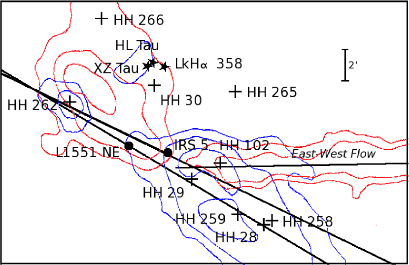
Figure 1: Diagram of the HH 262 region showing the location of HHs and YSOs. The contours correspond to the blueshifted and redshifted CO emission from the three molecular outflows identified in the region (two outflows in the NE-SW direction, associated with the YSOs L1551 IRS 5 and L1551 NE, and the east-west outflow; Moriarty-Schieven et al. 2006). The straight lines are drawn along the outflow axes.

2 Observations and Data Reduction

Observations of HH 262 were made on 22 November 2004 with the 3.5-m telescope of the Calar Alto Observatory (CAHA). Data were acquired with the Integral Field Instrument Potsdam Multi-Aperture Spectrophotometer PMAS (Roth et al., 2005) using the PPAK configuration that has 331 science fibres, covering an hexagonal FOV of 74$\times$65 arcsec² with a spatial sampling of 2.7 arcsec per fibre, and 36 additional fibres to sample the sky (see Fig. 5 in Kelz et al. 2006). The I1200 grating was used, giving an effective sampling of 0.3 Å pix^-1 ($\sim 15$ km s^-1 for H$\alpha$) and covering the wavelength range $\sim 6500$–7000 Å, thus including characteristic HH emission lines in this wavelength range (H$\alpha$, [N ii] $\lambda\lambda$6548, 6584 Å  and [S ii] $\lambda\lambda$6716, 6731 Å). The spectral resolution (i. e. instrumental profile) is $\sim 2$ Å  FWHM ($\sim 90$ km s^-1) and the accuracy in the determination of the position of the line centroid is $\sim 0.2$ Å  ($\sim 10$ km s^-1 for the strong observed emission lines). Eight overlapped pointings of 1800-s exposure time each were observed to obtain a mosaic of $\sim$ 1.5 $\times$ 3 arcmin² to cover almost the entire emission from HH 262. Note, however, that this mosaic does not cover the extended, arc–shaped emission known as HH 262E, which is most probably related to HH 262. In Table 1 we list the centre positions of each pointing and the corresponding HH 262 knot identification following the nomenclature of Garnavich, Noriega-Crespo & Green (1992), extended by López et al. (1995).

Data reduction was performed using a preliminary version of the R3D software (Sánchez, 2006), in combination with IRAF and the Euro3D packages (Sánchez, 2004). The reduction consists of the standard steps for fibre-based integral field spectroscopy. A master bias frame was created by averaging all the bias frames observed during the night and subtracted from the science frames. The location of the spectra in the CCD was determined using a continuum-illuminated exposure taken before the science exposures. Each spectrum was extracted from the science frames by co-adding the flux within an aperture of 5 pixels along the cross-dispersion axis for each pixel in the dispersion axis, and stored in a row-stacked-spectrum (RSS) file (Sánchez, 2004). At the date of the observations we lacked of a proper calibration unit for PPAK. Therefore the wavelength calibration was performed iteratively, following all the steps described in López et al. (2008) for HHL 73, another target of our HH IFS survey. The final wavelength solution was set by using the sky emission lines found in the observed wavelength range. The accuracy achieved for the wavelength calibration was better than $\sim 0.1$ Å ($\sim 5$ km s^-1). Observations of a standard star were used to perform a relative flux calibration. A final datacube containing the 2D spatial plus the spectral information of HH 262 was then created from the 3D data by using Euro3D tasks to interpolate the data spatially until reaching a final grid of 2.16 arcsec of spatial sampling and with a spectral sampling of 0.3 Å . Further manipulation of this datacube, devoted to obtain integrated emission line maps, channel maps and position–velocity maps, were made using several common-users tasks of STARLINK, IRAF and GILDAS astronomical packages and IDA (García-Lorenzo, Acosta-Pulido & Megias-Fernández, 2002), an specific IDL software to analyse 3D data.

Table 1: Positions of the single pointings of the HH 262 mosaic.

Position		knot
04h31m58$\aas@@fstack{s}7$	+18$\degr$12$\arcmin$07$\arcsec$	GH9
04h32m01$\aas@@fstack{s}1$	+18$\degr$12$\arcmin$35$\arcsec$	K18
04h32m00$\aas@@fstack{s}5$	+18$\degr$12$\arcmin$05$\arcsec$	K19
04h32m00$\aas@@fstack{s}9$	+18$\degr$11$\arcmin$53$\arcsec$	K20
04h32m00$\aas@@fstack{s}1$	+18$\degr$11$\arcmin$33$\arcsec$	GH10W
04h32m01$\aas@@fstack{s}1$	+18$\degr$11$\arcmin$24$\arcsec$	GH10E
04h32m00$\aas@@fstack{s}0$	+18$\degr$11$\arcmin$17$\arcsec$	K26
04h31m59$\aas@@fstack{s}7$	+18$\degr$10$\arcmin$30$\arcsec$	K22

3 Results

3.1 Integrated line-emission maps

3.1.1 Emission line images

Emission from H$\alpha$ and [S ii] $\lambda\lambda$6716, 6731 Å  was detected in all the mapped region. In contrast, emission from the [N ii] $\lambda\lambda$6548, 6584 Å lines was not detected, except in the knot GH9, towards the northwestern side of HH 262. Narrow-band images for each of the lines were generated from the datacube. For each position, the flux of the line was obtained by integrating the signal over the whole wavelength range covered by the line and subtracting the continuum emission obtained from the wavelengths adjacent to the line. The narrow-band maps of HH 262 obtained in this way are shown in Fig.2

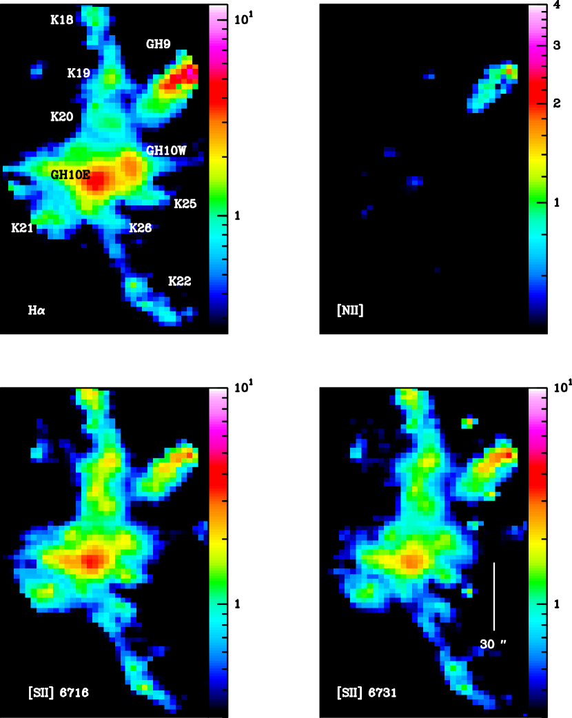
Figure 2: Integrated maps of the HH 262 emission obtained from the datacube by integrating the signal within the wavelength range including the line labelled in each panel: (H$\alpha$ : $\lambda$6558–6569 Å, [N ii] : $\lambda$6580–6586 Å, [S ii] : $\lambda$6716 6712–6719 Å  and [S ii] : $\lambda$6731 6728–6734 Å). Fluxes have been displayed in a logarithmic scale, in units of 10^-16 erg s^-1 cm^-2. In all the maps, north is up and East is to the left. The HH 262 knots have been labelled in the H$\alpha$ panel

As can be seen from the panels of the figure, the H$\alpha$ and [S ii] emissions reveal a similar morphology, although the emission of some the knots is stronger in [S ii] than in H$\alpha$, while the brightness of the [S ii] and H$\alpha$ emission is similar for the other knots, in good agreement with the results found in previous CCD narrow-band images (Garnavich, Noriega-Crespo & Green 1992).

Our IFS data allow us to obtain the first [N ii] narrow-band image of HH 262. Because there are no CCD images acquired through a line filter with a passband narrow enough to isolate the [N ii] lines from H$\alpha$, the morphology of HH 262 in the [N ii] lines has remained unknown up to now. Note that the morphology of HH 262 in [N ii]  is different than in H$\alpha$ and [S ii] : i. e. HH 262 does not show its characteristic ”hour-glass” structure because the emission from [N ii] was detected only in knot GH9. In the other knots, [N ii] emission was only marginally detected or not detected at all.

3.1.2 Kinematics

Radial velocity maps for the H$\alpha$ and [S ii] emissions were obtained from the line centroids of a Gaussian fit to the line emission. All the HH 262 knots show redshifted velocities in both lines (H$\alpha$ and [S ii]), the velocity field being rather complex (Figure 3). The velocities derived for the H$\alpha$ emission range from $\sim+25$ to $\sim+85$ km s^-1 and, in general, are $\sim 20$ km s^-1 lower than those derived from [S ii] emission, which range from $\sim+40$ to $\sim+110$ km s^-1, the difference found between the H$\alpha$ and [S ii] velocities being reliable. The highest velocities are found towards the central knots of HH 262 (a velocity of $\sim+70$ in H$\alpha$ and and $\sim+100$ km s^-1 in the [S ii] $\lambda$ 6716 Å line, respectively, is found around GH10W). The velocity decreases as we move north and south of the centre, with a steeper decrease towards the north. The lowest velocities appear towards the northwest, in the GH9 knots, where a value of $\sim+30$ km s^-1 for both lines is derived around its northern edge. It is interesting to note here that the velocities derived in this work are in good agreement with those found in previous studies (from long-slit spectroscopy of Graham & Rubin 1992, and from Fabry-Perot observations of López et al. 1998).

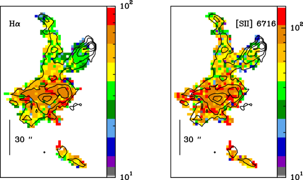
Figure 3: Velocity maps of the line centroid. Velocities (km s^-1) are referred to the $V_{\mathrm{LSR}}$ of the parent cloud. Contours of the integrated flux of the H$\alpha$ line have been overlaid to help with the knots identification.

The FWHMs of the H$\alpha$ and [S ii] lines, obtained from the Gaussian fit and corrected from the instrumental profile, show the same behaviour: for both emissions, the widest FWHM values are found towards the centre of HH 262 ($\sim 80$ km s^-1 around the knot GH10E and $\sim 100$ km s^-1 around GH10W), the line widths diminishing when we move towards the north, reaching values of $\sim 30$ km s^-1 around the knot 18. The FWHMs vary along GH9, ranging from $\sim 40$ km s^-1 (similar to those found around knots 19 and 20) in the southern region of GH9, and increase towards the north (a FWHM of $\sim 65$ km s^-1 is found around the GH9 NE edge).

3.1.3 Physical conditions

Line-ratio maps of the integrated line emission were derived to explore the spatial behaviour of the electron density (from [S ii] 6716/6731) and the excitation conditions (from [S ii]/H$\alpha$ and from [N ii]/H$\alpha$ at the loci where [N ii] emission was detected).

As a general trend, the electron density ($n_{\mathrm{e}}$) derived in HH 262 is low when compared with densities found in most of the HH jets. The highest $n_{\mathrm{e}}$ values are found in GH9, coinciding with the HH 262 loci where emission from [N ii] was detected ($n_{\mathrm{e}}=490$–1000 cm^-3, increasing from the southeast to the northwest along GH9). The electron density decreases as we move towards the centre of HH 262, from north ($n_{\mathrm{e}}=270$ cm^-3 around K18) to south ($n_{\mathrm{e}}=100$ cm^-3 around K20). For the central knots (GH10E, GH10W and K25), the electron density lies close to the low-density limit of the [S ii] 6716/6731 line ratio sensitivity and thus only an upper limit for $n_{\mathrm{e}}$ of 30–50 cm^-3 was estimated. The electron density increases slightly as we move from the centre towards the south ($n_{\mathrm{e}}=120$cm^-3 around K22) and southeast ($n_{\mathrm{e}}=230$ cm^-3 around K21). These values were derived from the [S ii] 6716/6731 ratio, using the TEMDEN task of the IRAF/STSDAS package, and assuming $T_{\mathrm{e}}=10^{4}$ K.

The derived spatial distribution of the [S ii]/H$\alpha$ line ratio indicates that the excitation increases from east to west across HH 262. The lower line ratio values ([S ii]/H$\alpha\simeq$0.6–0.9) are found towards the western region of knots GH10W and GH9, reaching the lowest value (highest excitation) around GH9, coinciding with the loci where [N ii] emission is detected. Furthermore, the trend found is the [S ii]/H$\alpha$ line ratio decreases from the northern K18–20 knots (with [S ii]/H$\alpha\simeq$ 1.8–2.2) to the centre of HH 262 (GH10W-E knots, where [S ii]/H$\alpha\simeq$ 0.7–1.0). Beyond the centre of HH 262, the [S ii]/H$\alpha$ line ratio increases slightly (the gas excitation decreases) as we move to the southern knots (K22, where [S ii]/H$\alpha\simeq$ 1.2).

As already mentioned, the [N ii] emission appears very weak and it was detected only marginally in the brightest HH 262 central knots (see Fig. 2). To provide better confirmation of this result, we have analysed an integrated spectrum of each knot, obtained by co-adding the signal of the spaxels inside the aperture encircling the corresponding knot emission (see Section 3.3), thus improving the SNR and the depth of the spectra. From these spectra, we have derived values for the [N ii] flux emission (or an upper limit). Table 2 lists the flux of the [N ii] emission relative to the rms of the spectrum, the [N ii]/H$\alpha$ line ratio and its estimated error percentage. From the table, we can see that [N ii]/H$\alpha$ line ratios of $\sim$0.2 were obtained along GH9 knot. For the northern knots (K18, K19 and K20), we estimated an upper limit of $\sim$0.1 for this ratio (by considering the [N ii] flux emission enhancement at a 3$\sigma$ rms level). For the central (GH10) and southern (K21, K26 and K22) knots, [N ii] flux emission over the 3$\sigma$ rms level was not detected at all.

Table 2: Derived values for the [NII] knots emission

knot		[NII]/rms	[NII]/H$\alpha$	[NII]/H$\alpha$ error (%)
K18		$<$3.0	$<$0.10
K19		¡3.0	¡0.15	10
K20		¡3.5	¡0.18	18
	K20N	$<$3.0	$<$0.10
	K20S	¡4.0	¡0.18	17
GH9		¡3.5	¡0.22	18
	GH9N-shell	¡3.8	¡0.20	18
	GH9W	¡5.2	¡0.17	15
	GH9E	¡5.6	¡0.20	15
GH10W		$<$3.0	$<$0.05
GH10E		$<$3.0	$<$0.08
K21		$<$3.0	$<$0.10
K26		$<$3.0	-
K22		$<$3.0	-

We have searched the literature looking for HH spectra that would be similar to those extracted for the HH 262 knots. Low [N ii]/H$\alpha$ line ratios ($\sim$ 0.1–0.2), similar to those derived from the spectra of the HH 262 knots K19, K20 and GH9, have been measured in the spectra of known HH jets (e. g. HH 49,50: Schwartz & Dopita 1980; HH 111L: Morse et al. 1993; HH 123: Reipurth & Heathcote 1990; HH 126B: Ogura & Walsh 1991; HH 34 (apex): Morse et al. 1993). However, the spectra of these jet knots, covering a wider wavelength range to include other emission lines, seem to be quite different when compared with the HH 262 extracted spectra, and would thus trace gas at different conditions. For example, the [S ii]/H$\alpha$ ratios in these jet knots are in general lower than the [S ii]/H$\alpha$ ratio derived in the HH 262 knots having similar [N ii]/H$\alpha$ values, and the derived $n_{\mathrm{e}}$ of these jet knots are also higher than the densities derived for HH 262. Moreover, most of the above-mentioned knot spectra show emission from [O iii] lines. Although the IFS data of HH 262 analysed here do not cover a wavelength range that includes the [O iii] lines, it should be mentioned that we failed to detect [O iii] emission at the location of HH 262 in a CCD image of 3000-s exposure time, acquired through an appropriate narrow-band filter in a previous observing run. Thus, the HH 262 spectra appear to have lower excitation than the knots mentioned before having similar [N ii]/H$\alpha$ line ratios.

In order to compare the line ratios obtained in HH 262 with current models of shock-ionization, it has to be noted that the HH 262 fluxes have not been corrected for reddening. Thus the derived line ratios are somewhat affected by differential extinction. However, since the wavelengths of the lines considered are close, we expect that the differences between the observed and the corrected line ratios are not critical for model comparison. For instance, for other HH objects where corrected fluxes are available, the differences found are lower than 1 % and 15 % for the [N ii]/H$\alpha$ and [S ii]/H$\alpha$ ratios respectively (see e. g. Raga, Böhm & Cantó 1996 and references therein).

Line ratios such as those derived from the HH 262 spectra can be reproduced in a framework of shocks with slow shock velocities. To predict the expected line ratios of characteristic HH emission lines, Hartigan, Raymond & Hartmann (1987) modelled HH bow shocks for a wide range of shock velocities ($V_{\mathrm{s}}$), pre-shock densities and pre-shock ionization conditions, assuming radiative planar shocks. Equilibrium preionization models in the low density regime ($n_{\mathrm{e}}$ $\simeq$ 100–1000 cm^-3) and with low shock velocities ($V_{\mathrm{s}}$ $\leq$ 40 km s^-1 ) give low [N ii]/H$\alpha$ line ratios ($\sim$ 0.01–0.22, increasing with $V_{\mathrm{s}}$, with a weak dependence on the electron density) and high [S ii]/H$\alpha$ line ratios ($\sim$ 2.5–0.8, decreasing with $V_{\mathrm{s}}$). Thus [N ii]/H$\alpha$ ($\simeq$ 0.2) and [S ii]/H$\alpha$ ($\simeq$ 0.6) line ratios, such as those found in the GH9 knot, are compatible with those obtained in shock models with $V_{\mathrm{s}}$ $\simeq$ 30–40 km s^-1 occurring in a low density and partially ionized medium. Shock models with higher shock velocities ($V_{\mathrm{s}}\geq 60$ km s^-1) predict [S ii]/H$\alpha$ line ratios much lower (by a factor of 4), not compatible with the values derived in HH 262, even considering that the fluxes were uncorrected for reddening. Lower [N ii]/H$\alpha$ line ratios ($\sim$ 0.01) are found in the planar shock models with lower velocities ($V_{\mathrm{s}}$ $\sim$ 20 km s^-1). The line ratio values derived in the central knots GH10E-W show a trend that seems to be compatible, within the errors, with that found in shock models of very low $V_{\mathrm{s}}$. The [S ii]/H$\alpha$ line ratios derived in HH 262 are also well reproduced by the low-velocity ($V_{\mathrm{s}}\leq 40$ km s^-1) models of Hartigan, Morse & Raymond (1994) that include the effect of the magnetic field, for low $B$ values ($\sim 30$ $\mu$G, in accordance with the current estimates for the Taurus Molecular Cloud, Nakamura & Li 2008), and low ionization fractions ($x_{\mathrm{e}}\leq 0.1$).

3.2 Channel maps

Since the HH 262 emission spreads over a wide range of velocities, we will explore whether the complex, knotty HH 262 morphology shown in the narrow-band images is also found in all the channel maps or, on the contrary, there are changes in morphology depending on the velocity.

3.2.1 Spatial distribution of the emission

A more detailed sampling of the gas kinematics was obtained by slicing the H$\alpha$ and [S ii] emission of the datacube into a set of velocity channels. Each slice was made for a constant wavelength bin of 0.3 Å, corresponding to a velocity bin of $\sim 14$ km s^-1 (13.7 km s^-1 and 13.4 km s^-1 for H$\alpha$ and [S ii] respectively). The channel maps obtained for H$\alpha$ and [S ii] $\lambda$6716 Å are shown in Figs. 4 and 5 respectively.

From these maps, it can be seen that the emission spreads over velocity ranges of $\sim 290$ km s^-1 and $\sim 240$ km s^-1 wide for the H$\alpha$ and [S ii] $\lambda$6716 Å emissions, respectively. The HH 262 ”hour-glass” structure is found for redshifted velocities ranging from $\sim+5$ to $\sim+100$ km s^-1 in H$\alpha$, and from $\sim+30$ to $\sim+125$ km s^-1 in [S ii] $\lambda$6716 Å . Furthermore, the channel maps also show that the northern (K18, K19 and K20) and northwestern (GH9) knots have emission at lower velocities as compared with the other HH 262 knots. These knots show emission at blueshifted velocities (up to $\sim-50$ km s^-1) in contrast with the southern HH 262 knots (K22), whose emission just begins to appear at velocities close to the rest velocity of the ambient cloud. Note in particular that the bright knot GH9 does not show significant emission for velocities higher than $\sim+100$ km s^-1, while the emission from the central (GH10E-W) and southern (K22) knots reach velocities up to $\sim$+180 km s^-1 and $\sim$+150 km s^-1 respectively. For GH9 and the northern knots, the strongest emission corresponds to the velocity channels ranging from $\sim+19$ to $\sim+45$ km s^-1 in H$\alpha$, and from $\sim+30$ to $\sim+55$ km s^-1 in [S ii] . In contrast, for the central GH10E-W knots, the strongest emission appears at higher velocities (in channels ranging from $\sim+60$ to $\sim+90$ km s^-1 in H$\alpha$, and from $\sim+70$ to $\sim+110$ km s^-1 in [S ii] ). Thus, we found signatures of deceleration of the optical emission as we move to the north, away from the exciting source of the molecular outflow. Furthermore, an increase of the density in the northwestern GH9 knot relative to the rest of the HH 262 could also be contributing to the deceleration of the outflow and thus derive lower velocities for the GH9 region.

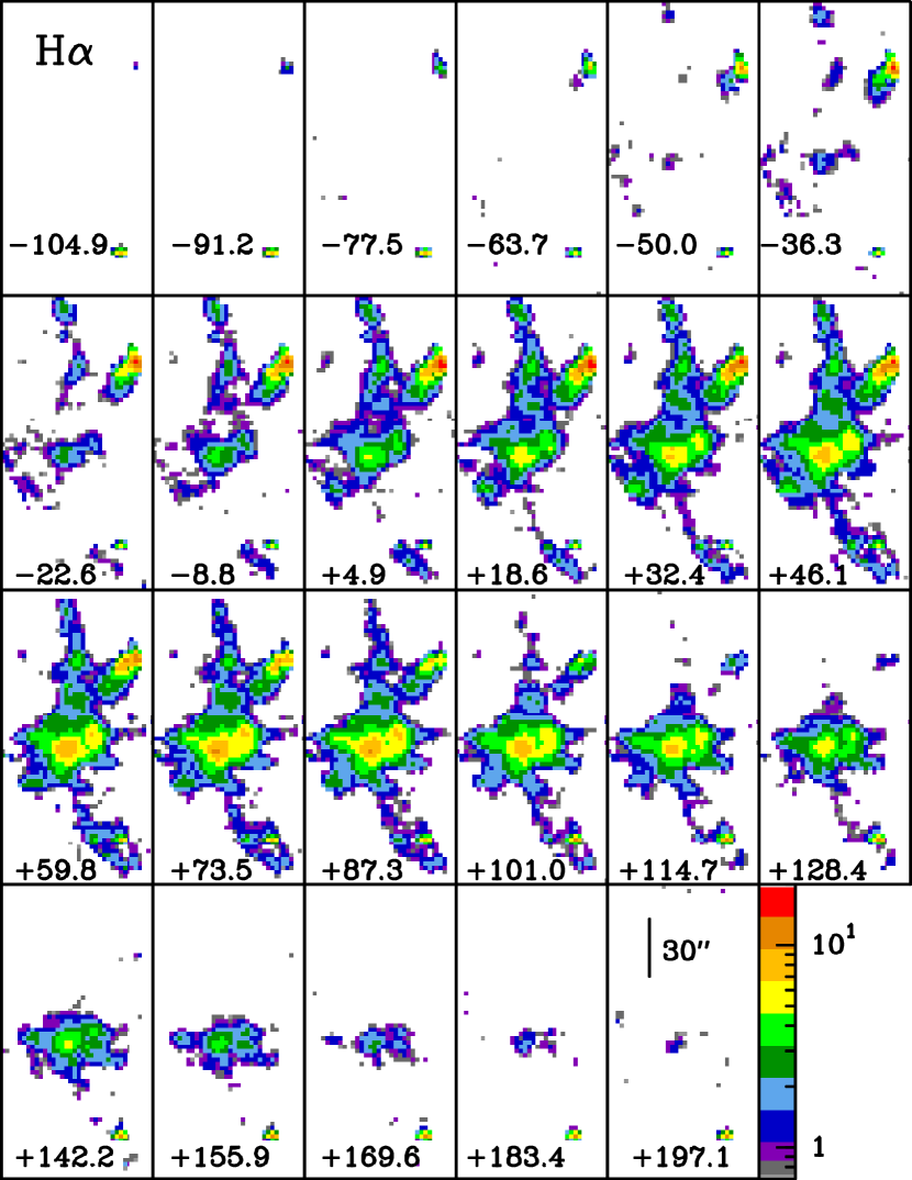
Figure 4: H$\alpha$ channel maps centred on the $V_{\mathrm{LSR}}$  radial velocities (km s^-1) labelled in each panel. The spatial scale is given in one of the panels. Fluxes have been displayed in a logarithmic scale, in units of $10^{-16}$ erg s^-1 cm^-2.

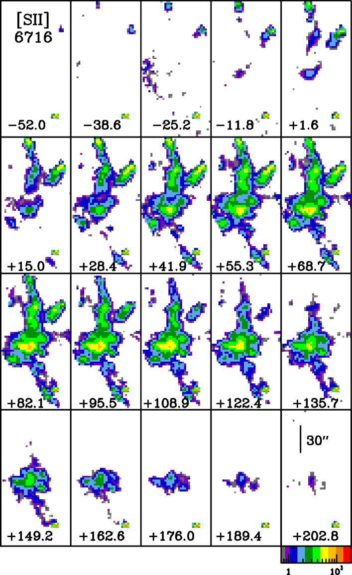
Figure 5: Same as Fig. 4, but for the [S ii] 6716 Å  emission line.

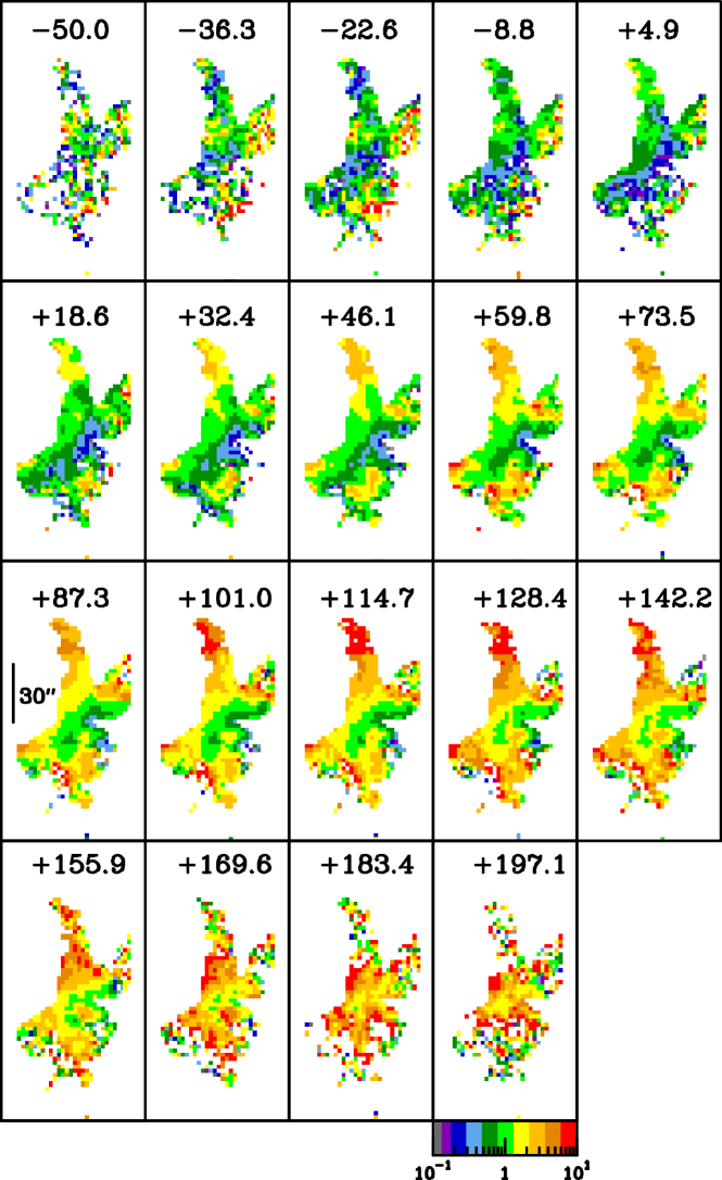
Figure 6: The [S ii]/H$\alpha$ line-ratio maps derived from the channel maps at the velocities labelled in the corresponding panel.

3.2.2 Density and excitation conditions

The behaviour of the density and excitation as a function of velocity was explored by generating the appropriate line-ratio channel maps.

We did not find evidence of density variations as a function of velocity in HH 262, as the [S ii] 6716/6731 line-ratio channel maps show a similar pattern for all the velocity bins. The [S ii]/H$\alpha$ line-ratio channel maps are displayed in Fig.  6. The maps in Fig.  6 show a trend of an increasing [S ii]/H$\alpha$ line ratio (i. e. a decreasing excitation) with increasing velocity. Regarding the spatial distribution, the general trend found for each velocity channel is a decrease in the line ratios (i. e. an increase in the excitation) from east to west across HH 262. In fact, the behaviour found in the integrated line-ratio map, where the highest excitation (lowest line-ratio values) is found along the western edge of knots GH9 and GH10W, is also found for each velocity channel.

3.3 The spectral atlas of HH 262

A more careful inspection of the HH 262 IFS narrow-band images (Fig. 2) shows the very complex morpholohy already found in the CCD images with higher spatial resolution: most of the named HH 262 knots appear to be quite extended and can be resolved into substructures (e. g.  GH9). As already mentioned, IFS data are well suited to characterizing the spectral properties of such as complex morphology in a more efficient way that by using long-slit observations. To take advantadge of this, we performed a more detailed spectral atlas of HH 262. First of all, we obtained a representative spectrum for each knot by co-adding the IFS spectra extracted from the spaxels inside an appropriate aperture encircling the emission of the HH 262 knot. The size of the apertures and the number of spectra that were co-added to obtain the representative spectrum of the knot, are listed in Table 3.

Table 3: Apertures defined for the extraction of the knot spectra.

knot		Aperture	Spectra
		(arcsec)$\times$(arcsec)
K18		115.$\times$14.5	46
K19		18.5$\times$15.5	27
K20		111.$\times$13.5	30
	K20N	14.5$\times$6.51	5
	K20S	18.5$\times$6.51	12
GH9		113.$\times$34.5	96
	GH9N-shell	12.5$\times$24.5	11
	GH9W	15.5$\times$7.51	9
	GH9E	18.5$\times$15.5	28
GH10W		17.5$\times$13.5	20
GH10E		17.5$\times$14.5	51
K21		17.5$\times$4.51	8
K26		19.5$\times$5.51	10
K22		111.$\times$13.5	31
	K22N	16.5$\times$7.51	11
	K22C	16.5$\times$8.51	12
	K22S	16.5$\times$4.51	5

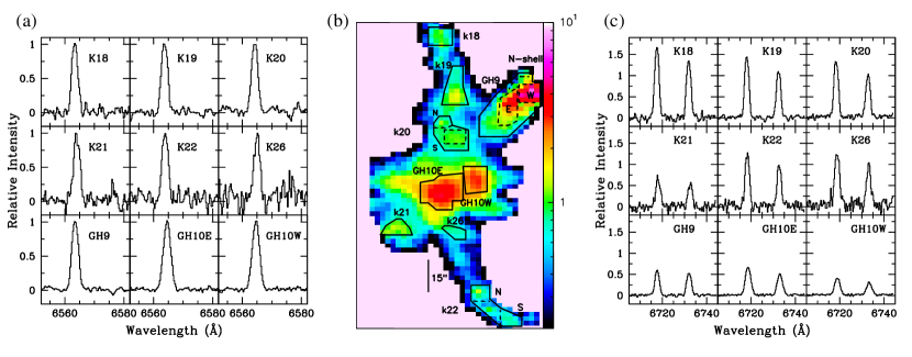
Figure 7: Spectra of the HH 262 knots in the spectral windows including H$\alpha$+[N ii] (a) and [S ii] 6716,6731 emission lines (c). Each spectrum has been obtained by co-adding the spectra of the spaxels inside an aperture (continuous box) including the knot emission, and its intensity has been normalized to the H$\alpha$ peak intensity. The apertures have been marked and labelled over the H$\alpha$ map of HH 262 (b) and listed in Table 3. Dashed boxes correspond to the substructures defined inside a given knot.

Figure 8: HH 262 spectra in the [S ii] spectral window extracted from individual spaxels along a longitudinal axis. Spectra are displayed from north (top left) to south (bottom right). Each spectrum corresponds to an aperture of 2.16 $\times$ 2.16 arcsec² and has been normalized to the H$\alpha$ peak intensity. The knot where the spectrum was extracted is indicated in the corresponding panel. For each spectrum, the position within HH 262 is indicated by the ($\alpha$, $\delta$) offset in pixel units (2.16 arcsec pixel^-1) from the reference position. The reference (0,0) position has been set in the H$\alpha$ peak position of GH10E.

Figure 9: Same as Fig. 8, but for the spaxels of a cut along the transversal, nortwest-southeast HH 262 axis (from top left to bottom right).

Fig. 7 displays the spectra of the HH 262 knots, obtained in such a way, in the spectral windows covering the H$\alpha$ + [N ii] (left panel) and [S ii] (right panel) wavelength ranges. In order to make easier comparisons between the lines in the two spectral windows, the intensities in each of the spectra were normalized to the corresponding H$\alpha$ peak intensity. A quick inspection of the spectra in the two spectral windows suggests that the excitation conditions significantly vary from knot to knot. Note in particular that the spectrum extracted at the northern knot (K18) presents the highest [S ii]/H$\alpha$ line ratio (this indicating the lowest gas excitation). Concerning the line profiles, a more careful inspection of the spectra suggests that the line profiles also vary from knot to knot. In particular, it can be appreciated that the southern (K21, K22 and K26) and central (GH10W-E) knots show more complex, asymmetric line profiles than the northern (K18, K19) knots for both the H$\alpha$ and [S ii] lines.

Furthermore, in order to better visualize the spectral variations at a smaller spatial scale, both along and across HH 262, we extracted spectra of individual spaxels for two cuts made along the two main HH 262 axes. One cut was performed from north to south, intersecting emission from knots K18, K19, K20, GH10E and K22. The other cut, from northwest to southeast, intersects emission from knots GH9, GH10W, GH10E and K21. The position where the H$\alpha$ emission has the peak, at the central knot GH10E, was set as the origin of positions for referring the location of a given spectrum. The resulting spectra from these two cuts, in the [S ii] window and normalized to their H$\alpha$ peak intensities, are displayed in Figs. 8 and 9. The spectra displayed in these figures suggest there are variations in the kinematics and physical conditions (excitation and density) along and across HH 262 even on a short spatial scale ($\leq$ 3 arcsec), because we found appreciable differences, both in the line intensity and in the line profiles between the spectra extracted at adjacent spaxels. In particular, the longitudinal cut (Fig. 8) shows the already mentioned increasing in the gas excitation as we move from the north to the centre of HH 262, suggested by the decrease along this direction in the [S ii] line intensities relative to H$\alpha$. This cut also shows that, as a general trend, the line profiles for positions north of the central HH 262 knots are more symmetric and single-peaked as compared with those of the centre and south, where the profiles appear wider, suggesting in some cases a contribution from two velocity components, partially resolved at our spectral resolution. Such a regular trend is not observed in the transversal cut (Fig. 9), although the extracted spectra reinforced the finding of the short spatial-scale variation conditions across HH 262.

3.3.1 Remarks on selected knots

As has already been mentioned, the H$\alpha$ and [S ii] narrow-band images of HH 262 show that the emission from some knots appears split into subcondensations. Furthermore, some knots (e. g. K22 and the central GH10E-W knots) show more complex, asymmetric line profiles, suggesting a contribution from two velocity components at several positions, while the line profiles are found to be more symmetric and single-peaked in the other knots. Thus, in order to characterize better the kinematics and physical conditions in selected HH 262 knots, we also extracted spectra for each knot subcondensation (see Table 3 and Fig. 7, central panel for identification) in addition to the spectrum extracted for the whole knot emission.

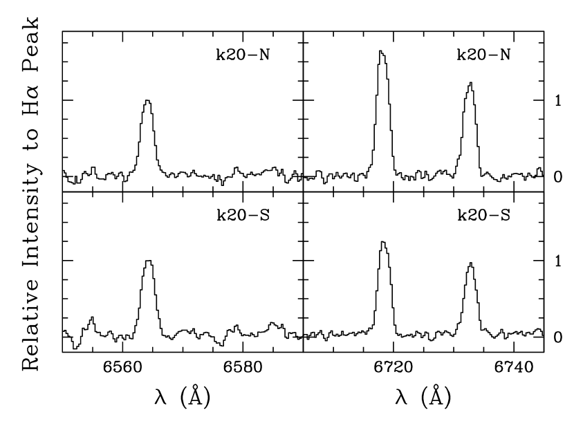
Figure 10: Spectra in the H$\alpha$+[N ii] (left) and [S ii] (right) windows of the two K20 knot subcondensations obtained by co-adding the IFS spectra extracted from the spaxels included in the apertures encircling the subcondensations. In the two windows, the intensity has been normalized to the corresponding H$\alpha$ peak intensity.

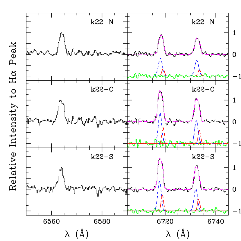
Figure 11: Same as Fig.10 but for K22. The fits to the [S ii] line profiles, obtained from the model, have been drawn in the right panel. The two velocity components are shown at the bottom. The residual, obtained by substracting the fit from the observed profile, is plotted in green.

Figure 12: Same as Fig. 10 but for GH9 knot.

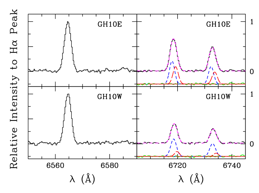
Figure 13: Same as Fig. 11 but for the GH10E-W knots.

• K20:

  Two subcondensations were morphologically defined in knot 20 (K20-N and K20-S), its peaks being found to be separated by $\sim$ 10 arcsec. We have not found appreciable kinematic differences between these two subcondensations. As can be seen in Fig. 10, the H$\alpha$ and [S ii] line profiles are both similar for the two subcondensations as well as the velocities derived from the centroid of these lines ($\sim$+60 km s^-1 and +85 km s^-1 respectively). In contrast, a significant change in the [S ii]/H$\alpha$ line ratios can be appreciated when comparing the spectra of the two K20 subcondensations, which traces an appreciable increase in the gas excitation as we move from north to south by only a few arcsec, suggesting a steep gradient of the gas excitation along K20.

• GH9:

  The IFS data indicate that the northwestern arm of HH 262 (i. e. GH9) seems to have different physical conditions compared to the other HH 262 knots. We extracted the spectra for two subcondensations (GH9W and GH9E) and also for the lower-brightness shell at the northern GH9 edge (N-Shell) (see Fig. 7 and Table 3 for identification). Their spectra are shown in Fig. 12. Concerning the kinematics, we did not find appreciable differences among the GH9 subcondensations. The line profiles appear to be single-peaked along the whole of GH9. The velocities derived from the line centroids are similar in the N-Shell and GH9W, being slightly higher (by $\sim$ 15  km s^-1) in GH9E. In contrast, we can appreciate changes in the physical conditions within GH9 as we move along the knot. Differences in the excitation conditions (increasing from N-Shell, GH9E to GH9W) are present as the [S ii]/H$\alpha$ line ratio variations indicate. Furthermore, the electron density also varies from one subcondensation to another. The highest $n_{\mathrm{e}}$ ($\sim$ 1000 cm^-3) is found in the N-Shell, decreasing to $n_{\mathrm{e}}$ $\sim$ 850 cm^-3) in GH9W and to $n_{\mathrm{e}}$ $\sim$ 600 cm^-3 in GH9E. Taking into account that $n_{\mathrm{e}}$ drop at the centre of HH 262 (i. e. around knots GH10E-W) until reaching values for which the [S ii] line ratio is not density sensitive in the central region, we can infer that there is a steep density gradient across HH 262 in the northwest direction.

• K22:

  K22 is one of the HH 262 knots whose extracted spectrum suggests that the line profiles are double-peaked. Morphologically, the knot appears curved, elongated and quite extended, but split into subcondensations. We extracted spectra for each of the three bright K22 subcondensations (K22-N, K22-C and K22-S, the separation between the K22-N and K22-S peaks being $\sim$ 10 arcsec). The spectra are shown in Fig. 11. There are appreciable differences in the [S ii]/H$\alpha$ line ratios among the K22 subcondensations, this being indicative of an increase in the gas excitation as we move from south to north along K22. Thus, a similar gradient in the gas excitation, but in the opposite direction to that found in K20, is detected along K22. The $n_{\mathrm{e}}$ derived from the [S ii] line ratio increases from south to north along K22, i. e. following the same trend that the gas excitation.

  Concerning the kinematics, both the H$\alpha$ and [S ii] line profiles of the three subcondensations appear asymmetric and would appear to be double-peaked. We used the [S ii] lines to perform a decomposition of the line profiles by applying a model with two Gaussian components. Gaussian fitting was perfomed using the DIPSO package of the STARLINK astronomical software. The wavelength difference between the two [S ii] lines was fixed according to their corresponding atomic parameters. The same FWHM of the Gaussian in each of the two [S ii] lines was assumed for each component of the profile. According to the fit parameters, we found two velocity components, both redshifted and with a peak separation of $\sim$ 50 km s^-1 between them. For both components, the trend found is the peak velocity increases from the southern to the northern subcondensation. The strongest component has lower redshifted peak velocities ($V_{\mathrm{LSR}}$ from +55 to +70 km s^-1 from south to north), while the faintest component has higher redshifted peak velocities ($V_{\mathrm{LSR}}$ from +105 to +120 km s^-1 from south to north). In Fig. 11 (right panel), we have also drawn the fits to the [S ii] line profiles obtained from the model. The two individual components are shown at the bottom. Residuals, obtained by subtracting the fit from the observed line, are also plotted.

• GH10:

  Fig. 13 displays the spectra of the central GH10E (top) and GH10W (bottom) knots in the H$\alpha$+[N ii] (left) and [S ii] windows. In the entire area analysed, the spectra extracted at each spaxel of the region covering these two central knots show broad and asymmetric line profiles, suggesting in most of the positions a double-peaked profile. We performed the line profile decomposition analysis described above (K22 subsection) in all the spaxels of this central region using the [S ii] doublet. From the fit, we found two redshifted velocity components spreading over the whole region, the component with the lower velocity being the strongest. We were unable to find a clear spatial separation between these two components that would allow the association of each of them with a given region of the central knots. However, a certain trend appears in which the higher-redshifted component is brighter towards the east of the GH10E knot, having its peak intensity somewhat displaced from the knot centre and showing in addition a secondary peak intensity in a region around the centre of GH10W. The lower-redshifted velocity component has the peak intensity in the regions located around the centre and southeast of GH10E.

  We show in Fig. 13 the fits to the [S ii] line profiles obtained from the model applied to the spectra, obtained as described in §3.3, of knots GH10E and GH10W. From the fit parameters, we found $V_{\mathrm{LSR}}$ of +60 and +120 km s^-1 for the two GH10E components and of +85 and +145 km s^-1 for these of GH10W knot.

4 Discussion and Conclusions

We have carried out a study of the kinematics and physical conditions of HH 262 based on IFS observations. From the analysis of these data we find:

• HH 262 shows a non-collimated, ”hour-glass” morphology in the H$\alpha$ and [S ii] lines. In contrast, the emission from the [N ii] lines is below detection limit except in the northwestern knot GH9. This work therefore presents the first narrow-band [N ii] image currently obtained of HH 262 to show its surprisingly different morphology as compared with the morpholgy found in the other characteristic HH emission lines.

• In all the HH 262 knots, radial velocities derived from the line centroids appear redshifted, relative to the cloud velocity. The highest velocities and FWHM values are found in the central knots.

• A more detailed picture of the kinematics was derived from the channel maps, which shows that the emission spreads over a wide range of velocities, the range slightly varying for the different knots. Furthermore, inspection of the HH 262 extracted spectra shows that there are broad, asymmetric line profiles at the southern (K22) and central knots (GH10E-W) that are double-peaked at several positions, which would suggest contribution from two velocity components. The line profiles appear more symmetric and single-peaked away from the centre, in the northern (K18–K20) and northwestern (GH9) knots.

• Concerning the physical conditions in HH 262, we found variations on a spatial scale of $\leq$3 arcsec (i. e. of the order of our spatial resolution). As a general trend, the electron densities, derived from the [S ii] line ratios, are low. In particular, only an upper limit could be set for the brightest, central HH 262 knots. Because $n_{\mathrm{e}}$ is referred to the density of the ionized gas, we propose that the only a small fraction of the atomic gas in HH 262 is ionized, the remainder being mostly neutral gas. It is also plausible that the total density of the gas is lower in this region because the evolved molecular outflow has had enough time to clear the medium. Over the entire velocity range of the emission, the gas excitation, derived from the [S ii]/H$\alpha$ line ratios, increases as we move towards the western region of knot GH10W and to knot GH9 i. e. moving towards the edges of HH 262 which are closer to the higher extinction region of the cloud. The general trend found is thus that the densest knots have the highest gas excitation and the lower centroid velocities.

All these characteristics of HH 262 derived from the IFS data reinforce the causal relationship of the optical line emission with the two molecular outflows (one powered by L1551-IRS5 and the other, by L1551 NE) found in the region were HH 262 is located. In fact, is widely accepted the association between HH 262 and the redshifted lobe of the L1551-IRS5 molecular outflow, first proposed by Rodríguez et al. (1989) and confirmed later on by the Fabry-Perot observations (López et al., 1998).

Detailed PV maps of the L1551-IRS5 outflow performed by Stojimirović et al. (2006) from high-sensitivity CO observations show a pattern that is characteristic of an evolved molecular outflow, according to current model simulations of the entrainment outflow mechanisms (Velusamy & Langer 1998, Richer et al. 2000). In the Stojimirović et al. (2006) PV CO maps, the HH objects are found associated with the molecular emission at the highest velocities, highlighting the interaction regions of the shocks at the head of the shock interface between the supersonic gas and the environment. In contrast, the CO emission at lower velocities appears as a limb-brightened shell-like emission. Thus, the result derived from the Stojimirović et al. (2006) work support the proposed scenario, in which the HH 262 emission traces the walls of a conical cavity evacuated by an evolved molecular outflow (L1551-IRS5). In such a scenario, one would expect that the HH 262 radial velocities to decrease (due to projection effects) as we move away from the axis outflow (i. e. from the central GH10 knots, where we found the highest integrated velocities, to the other knots). It is also expected to find double-peaked line profiles along the outflow axis (corresponding to material moving in the forward and rear faces of the cone) and a single-peaked profile away from the axis. Such a trend is observed in HH 262 from our IFS data, where the lines of the central knots appear with a complex, asymmetric line profiles, being double-peaked for most positions, while the line profiles of the knots farther away from the outflow axis (e. g. K18, K19 or GH9) appear more symmetric and single-peaked.

In addition to the L1551-IRS5 outflow, the blueshifted lobe of another younger, dimmer CO outflow, powered by L1551 NE, also encompases HH 262 (Moriarty-Schieven et al., 2006). Thus, HH 262 is located in a region where two molecular outflows are interacting (see Fig.1) and it is expected that this interaction gives signatures on the jet turbulence. This interaction could in part be responsible for the complex velocity pattern and the wide line profiles found in the optical emission lines. In a turbulent jet scenario, the highest FWHM values are expected to be found close to the axis, where there are contributions from gas within a wider range of velocities because we intersect the entire jet beam, while FWHM values would be lower at the edge of the jet, away from the axis. This is the trend found in the IFS HH 262 data for the FWHMs , where the highest values correspond to the central GH10 knots and decrease moving towards the edges of the emission.

The association of HH 262 with an evolved molecular outflow near the edge of a dark cloud would in part justify the low density values derived for most of the knots, as the outflow has cleared the medium. Note however that the density of the gas is probably higher than the density derived from the [S ii] line ratio, which is an indicator of only the density of the ionized fraction of the gas rather than of the total density (Sánchez et al. 2007).

Finally, let us discuss the new finding presented here concerning the low intensity of the [N ii] emission in HH 262. Such a behaviour has been found in slow-velocity shocks as those modelled by Hartigan, Raymond & Hartmann (1987). In particular, the [N ii]/H$\alpha$ and [S ii]/H$\alpha$ line ratios derived for the knot GH9 are fully compatible with those derived in shock models with $V_{\mathrm{s}}$ $\simeq$ 30–40 km s^-1 occurring in a low density, partially ionized medium. Lower [N ii]/H$\alpha$ line ratios ($\simeq$ 0.01) are found in models with lower $V_{\mathrm{s}}$ ($\leq$ 20 km s^-1 ), thus being compatible, within the errors, with the marginal detection of [N ii] in the northern knots and with the line ratios derived in those knots. The HH 262 line ratios are also compatible with those predicted by the shock models of Hartigan, Morse & Raymond (1994) for low magnetic field strength and low ionization fraction values. Note however that the morphology of HH 262 is too complex and rather different from the morphologies found in most known HH jets. Thus, it should not be expected that the radiative planar shock models of Hartigan, Raymond & Hartmann (1987) and Hartigan, Morse & Raymond (1994) succeeded in reproducing all the HH 262 properties derived from the current IFS data. Further IFS observations covering a wavelength range blueward of [N ii] + H$\alpha$ are needed to search for emission in the [N i] $\lambda$ 5200 Å line whose strength could justify the weakness of the [N ii] emission found in HH 262 provided the nitrogen abundance were not far from the solar value.

References

- Devine, Reipurth & Bally (1999) Devine D., Reipurth B., Bally J., 1999, AJ, 118, 972
- Emerson et al. (1984) Emerson J.P., Harris S., Jennings R.E., Beichman C.A., Baud B., Beinteman D.A., Marsden P.L., Wesselius P.R., 1984, ApJ, 278, L49
- García-Lorenzo, Acosta-Pulido & Megias-Fernández (2002) García-Lorenzo B., Acosta-Pulido J., Megias-Fernández E., 2002, in ASP Conf. Ser. 282, Galaxies: The Third Dimension, ed. M. Rosado, L. Binette, & L. Arias (San Francisco: ASP), 501
- Garnavich, Noriega-Crespo & Green (1992) Garnavich P.M., Noriega-Crespo A., Green P.J., 1992, A&A, 24, 99
- Graham & Heyer (1990) Graham J.A., Heyer M.H., 1990, PASP, 102, 972
- Graham & Rubin (1992) Graham J.A., Rubin V.C., 1992, PASP, 104, 730
- Hartigan, Raymond & Hartmann (1987) Hartigan, P., Raymond, J., Hartmann, L., 1987, ApJ, 316, 323
- Hartigan, Morse & Raymond (1994) Hartigan, P., Morse, J.A., Raymond, J., 1994, ApJ, 436, 125
- Kelz et al. (2006) Kelz A., Verheijen M.A.W., Roth M.M. et al., 2006, PASP, 118, 129
- López et al. (1995) López R., Raga A.C.,Riera A., Anglada G., Estalella R., 1995, MNRAS, 274. L19.
- López et al. (1998) López R., Rosado M., Riera A., Noriega-Crespo A., Raga A.C., Estalella R., Anglada G., Le Coarer E., Langarica R., Tinoco S., Cantó J., 1998, AJ, 116, 845
- López et al. (2008) López R., Sánchez, S.F., García-Lorenzo B., Gómez, G., Estalella R., Riera A., Busquet, G., 2008, MNRAS, 384, 464
- Moriarty-Schieven et al. (2006) Moriarty-Schieven G.H.,Johnstone D, Bally J., Jenn T., 2006, ApJ, 645, 357.
- Morse et al. (1993) Morse, J.A., Heathcote, S., Hartigan, P., Cecil, G., 1993, AJ, 106,1139
- Nakamura & Li (2008) Nakamura, F., Li, Z-Y, 2008, astro-ph 0804.4201
- Ogura & Walsh (1991) Ogura, K., Walsh, J.R., 1991, AJ, 101, 185
- Reipurth & Heathcote (1990) Reipurth, B., Heathcote, S., 1990 A&A, 229, 527
- Raga, Böhm & Cantó (1996) Raga, A.C., Böhm, K.-H., Cantó, J., 1996, RevMexAA, 32, 161
- Richer et al. (2000) Richer, J. S., Shepherd, D.S., Cabrit, S., Bachiller, R., Churchwell, E., 2000, in Protostars and Planets IV, ed. Mannings, A.P. Boss & S.S. Russell (Tucson: Univ. Arizona Press), 867.
- Rodríguez, Anglada & Raga (1995) Rodríguez L. F., Anglada, G., Raga A.C., 1995, ApJ, 454, L149
- Rodríguez et al. (1989) Rodríguez L. F., Cantó J., Moreno M.A., López J.A.,1989, Rev. Mex. Astron. Astrof., 17, 111
- Roth et al. (2005) Roth M. M., Kelz A., Fechner T., Hahn T., Bauer S.-M., Becker T., Böhm P., Christensen L., Dionies F., Paschke J., Popow E., Wolter D., Schmoll J., Laux U., Altmann W., 2005, PASP, 117, 620
- Sánchez (2004) Sánchez, S. F. 2004, AN, 325, 167
- Sánchez (2006) Sánchez, S. F. 2006, AN, 327, 850
- Sánchez et al. (2007) Sánchez, S. F., Cardiel, N., Verheijen, M.A.W., Martí-Gordon, D., Vilchez, J.M., Alves, J., 2007, A&A, 465, 207.
- Schwartz & Dopita (1980) Schwartz, R.D., Dopita, M.A., 1980, ApJ, 236,543
- Stojimirović et al. (2006) Stojimirović I., Narayanan G., Snell R.L., Bally J., 2006, Apj, 649, 280.
- Velusamy & Langer (1998) Velusamy, T., Langer, W.D., 1998, Nature, 392, 685