On the derivation of Fourier’s law in stochastic energy exchange systems

Abstract

We present a detailed derivation of Fourier’s law in a class of stochastic energy exchange systems that naturally characterize two-dimensional mechanical systems of locally confined particles in interaction. The stochastic systems consist of an array of energy variables which can be partially exchanged among nearest neighbours at variable rates. We provide two independent derivations of the thermal conductivity and prove this quantity is identical to the frequency of energy exchanges. The first derivation relies on the diffusion of the Helfand moment, which is determined solely by static averages. The second approach relies on a gradient expansion of the probability measure around a non-equilibrium stationary state. The linear part of the heat current is determined by local thermal equilibrium distributions which solve a Boltzmann-like equation. A numerical scheme is presented with computations of the conductivity along our two methods. The results are in excellent agreement with our theory.

1 Introduction

A key to a comprehensive derivation of transport properties starting from a microscopic theory is to identify the conditions under which scales in a macroscopic system. This problem is especially challenging for interacting particle systems. To establish the conditions under which scales separate is to provide an understanding as to how a large number of particles whose microscopic motion is described by Newton’s equations organise themselves in irreversible flow patterns at the macroscopic level.

In the context of thermodynamics, macroscopic equations such as Fourier’s heat law derive from conservation laws supplemented by phenomenological ones. The former concern say the conservation of mass or energy, and reflect the existence of the corresponding conservation laws at the level of Newton’s equations. Phenomenological laws on the other hand provide linear relations between the currents associated with the flow of conserved quantities and thermodynamic forces in the form of gradients of the conserved quantities, thereby introducing a set of transport coefficients. Though the values of these coefficients can be precisely measured and are usually tabulated for the sake of their use in the framework of applied thermodynamics, they cannot be otherwise determined without knowledge of the underlying dynamics. A first-principles based computation of the transport coefficients consequently requires a deep knowledge and understanding of the dynamics, as well as their statistical properties.

For this purpose, a common procedure in non-equilibrium statistical physics –see e.g. Uhlenbeck’s discussion of Bogoliubov’s approach to the description of a gas in [3] or van Kampen’s views on the role of stochastic processes in physics [4]– is to apply the two-step programme which consists of (i) identifying an intermediate level of description –a mesoscopic scale– where the Newtonian dynamics can be consistently approximated by a set of stochastic equations, and (ii) subsequently analyzing the statistical properties of this stochastic system so as to compute its transport properties.

The first part of this programme was successfully completed in a recent set of papers [1, 2], in which we introduced a class of Hamiltonian dynamical systems describing the two-dimensional motion of locally confined hard-disc particles undergoing elastic collisions with each other. Whereas the confining mechanism prevents any mass transport in these systems, energy exchanges can take place through binary collisions among particles belonging to neighbouring cells. Under the assumption that binary collisions are rare compared to wall collisions, it was argued that, as a consequence of the rapid decay of statistical correlations of the confining dynamics, the global multi-particle probability distribution of the system typically reaches local equilibrium distributions at the kinetic energy of each individual particle before energy exchanges proceed. This mechanism naturally yields a stochastic description of the time evolution of the probability distribution of the local energies in terms of a master equation to be described below. An important property in that respect is that the accuracy of this stochastic reduction can be controlled to arbitrary precision by simply tuning the system’s parameters.

In [1, 2], arguments were presented supporting the result that the heat conductivity associated with this master equation has a simple analytical form, given by the frequency of energy exchanges. In a sense, this result is similar to the fact that, for instance, uniform random walks describing tracer dynamics have diffusion coefficients given in terms of jump probabilities of the walkers. However, contrary to such systems, the stochastic system at hand lacks a special property which facilitates the derivation of such results, namely the gradient condition. A system obeys the gradient condition if there exists a local function such that the current, whether of mass or energy, can be written as the difference of this function evaluated at separate coordinates [5]. In such cases, the diffusion coefficient is determined through a static average only, and is therefore easy to compute. Given that our stochastic system does not verify the gradient condition, it is in fact remarkable that the heat conductivity should take such a simple form.

In this paper, we complete the second part of the programme described above and provide a systematic derivation of the heat conductivity associated with heat transport in the class of stochastic systems derived in [1, 2]. We justify in particular why, in spite of the fact that our systems do not obey the gradient condition, the heat conductivity can still be computed from the Green-Kubo formula through a static average only. We achieve this by an alternative method which consists in considering the stationary heat flux produced by a temperature gradient across the system. We suppose the system is a two-dimensional slab. Along the first dimension, the system has finite extension, with the corresponding borders in contact with stochastic thermal baths at different temperatures. The system may be taken to periodic along the second dimension. As a result, a temperature gradient develops along the first dimension, which induces a heat flux from the warmer border to the colder one. We then set up a scheme to compute the resulting non-equilibrium stationary state and obtain the linear relation connecting the temperature gradient to the heat flux. This scheme proceeds by consistently solving the Bogoliubov-Born-Green-Kirkwood-Yvon (BBGKY) hierarchy up to pair distributions through a type of Chapman-Enskog gradient expansion. As the heat current associated with our systems depends on neighbouring pairs only, the knowledge of the pair distribution function to first order in the temperature gradient makes possible the computation of the heat current in the linear regime and, consequently, that of the thermal conductivity, thereby completing the derivation of Fourier’s law.

Our theoretical results are furthermore supported by the results of direct numerical simulations of the stochastic system, with excellent agreement. Simulation methods of kinetic processes governed by a master equation have been extensively developed after Gillespie’s original work [6, 7]. Here we describe a method which accounts for continuous energy exchanges among all the pairs of neighbouring cells.

The paper is organised as follows. The master equation is described in section 2, with relevant definitions. Statistical objects are described in section 3, identifying equilibrium and non-equilibrium stationary states. Local temperatures are defined in section 4 and the energy conservation law derived, thereby identifying heat currents. Section 5 offers a first computation of the heat conductivity through the method of Helfand moments. An alternative computation is presented in section 6, solving the BBGKY hierarchy as sketched above. The numerical scheme for the computation of the heat conductivity is discussed in section 7, with a presentation of the results. Finally, conclusions are drawn in section 8.

2 Master equation

Consider a lattice of confining two-dimensional cells, each containing a single hard-disc particle, and such that particles in neighbouring cells may perform elastic collisions with each other, thereby exchanging energy. Such mechanical systems with hard-core confining mechanisms have recently been considered in [1, 2] (see figure 1). In these systems, one distinguishes the local dynamics from the interacting dynamics. On the one hand, the local dynamics are characterized by a wall-collision frequency, $\nu_{\mathrm{W}}$, which depends on the geometry of the confining cell as well as on the kinetic energy of the moving particles. On the other hand, the interacting dynamics are characterized by the frequency of binary collisions, i.e. the frequency of collisions between neighbouring particles, $\nu_{\mathrm{B}}$.

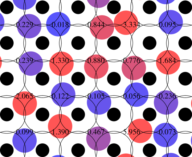
Figure 1: Snapshot showing an example of an interacting particle system with a confining mechanism, such as described in [2]. The coloured particles, colour-coded according to their kinetic energies from blue to red, move among an array of fixed black discs. The system has two parameters, the diameters of the fixed and moving discs. They are chosen so that their sum is larger than the distance between neighbouring fixed discs. This guarantees that the moving discs are trapped within their cells; their centers move within semi-dispersing billiards of bounded horizon (exterior intersection of the black circles). Though they are confined, the moving discs can nevertheless exchange energy through binary collisions as long as their diameters are properly chosen. The numbers indicate the values of the kinetic energies in every cell. In the limit where binary collisions are rare with respect to wall collisions, the energy exchange dynamics reduces to the stochastic evolution described by equation (1).

Under specific conditions, the scale separation, $\nu_{\mathrm{B}}\ll\nu_{\mathrm{W}}$, is achieved, which is to say that individual particles typically perform many collisions with the walls of their confining cells, rattling about their cages at higher frequency than that of binary collisions. In this regime, Liouville’s equation governing the time evolution of phase-space densities reduces to a master equation for the time evolution of local energies. Moreover the validity of this reduction is controlled by the scale separation between the two collision frequencies $\nu_{\mathrm{B}}$ and $\nu_{\mathrm{W}}$, and becomes exact in the limit of vanishing binary collision frequency. On the contrary, in the absence of a clear separation between binary and wall collision frequencies, the dynamics is not reducible to such a stochastic description and cannot be addressed in the context of this paper –see [2] for a discussion of that limit.

Throughout this article, we assume the validity of the scale separation between the wall and binary collision frequencies and focus on the stochastic reduction of the energy exchange dynamics, considering, as our starting point, the mesoscopic level description of the time evolution of probability densities as a stochastic evolution. The time evolution is thus specified by a master equation which accounts for the energy exchanges between neighbouring cells. Note that the dimensionality of the dynamics specifies the maximum dimension of the energy cell array we may consider. In the case of the dynamics depicted in figure 1, the array of energy variables would be two-dimensional. However, without loss of generality, we can simplify the description and consider instead a one-dimensional array according to which every cell has two neighbours instead of four, one on each side. A similar construction can be carried out in three dimensions, starting with systems of confined hard balls.

We can thus leave aside the underlying dynamics and consider instead a system of $N$ cells along a one-dimensional axis with energies $\{\epsilon_{1},\dots,\epsilon_{N}\}$ and let $P_{N}(\epsilon_{1},\dots,\epsilon_{N},t)$ denote the time-dependent energy distribution associated with this system. The time evolution of this object is specified according to

$$\hbox to0.0pt{\hss${}\partial{}$}_{t}P_{N}(\epsilon_{1},\dots,\epsilon_{N},t)=$$ (1)

$$\sum_{a=1}^{N}\int\/\mathrm{d}\/\eta\Big{[}W(\epsilon_{a}+\eta,\epsilon_{a+1}-\eta|\epsilon_{a},\epsilon_{a+1})P_{N}(\dots,\epsilon_{a}+\eta,\epsilon_{a+1}-\eta,\dots,t)$$

$$\hskip 49.79231pt-W(\epsilon_{a},\epsilon_{a+1}|\epsilon_{a}-\eta,\epsilon_{a+1}+\eta)P_{N}(\dots,\epsilon_{a},\epsilon_{a+1},\dots,t)\Big{]}\,,$$

where, for the sake of the argument, we assume periodic boundary conditions and identify cells $a=N+1$ and $a=1$.

The kernel $W$ specifies the energy transition rates, whereby a pair of energies $\{\epsilon_{a},\epsilon_{b}\}$ exchange an amount $\eta$ of energy. In the case of systems such as shown in figure 1, it is given by

$$W(\epsilon_{a},\epsilon_{b}|\epsilon_{a}-\eta,\epsilon_{b}+\eta)=\frac{2\rho_{\mathrm{m}}m^{2}}{(2\pi)^{2}|\mathcal{L}_{\rho,\rho_{\mathrm{m}}}(2)|}\int\/\mathrm{d}\/\phi\/\mathrm{d}\/\bi{R}\int_{\hat{\bi{e}}_{ab}\cdot\bi{v}_{ab}>0}\/\mathrm{d}\/\bi{v}_{a}\/\mathrm{d}\/\bi{v}_{b}$$ (2)

$$\hbox to0.0pt{\hss${}\times{}$}\hat{\bi{e}}_{ab}\cdot\bi{v}_{ab}\,\delta\left(\epsilon_{a}-\frac{m}{2}v_{a}^{2}\right)\delta\left(\epsilon_{b}-\frac{m}{2}v_{b}^{2}\right)\delta\left(\eta-\frac{m}{2}[(\hat{\bi{e}}_{ab}\cdot\bi{v}_{a})^{2}-(\hat{\bi{e}}_{ab}\cdot\bi{v}_{b})^{2}]\right)\,,$$

where $\hat{\bi{e}}_{ab}$ denotes the unit vector joining particles $a$ and $b$ with respective velocities $\bi{v}_{a}$ and $\bi{v}_{b}$, $\phi$ is the angle between the direction of this unit vector and a reference axis, $\bi{R}$ denotes the position of the center of mass of the two particles, $m$ their masses, $\rho_{\mathrm{m}}$ their radii, and $|\mathcal{L}_{\rho,\rho_{\mathrm{m}}}(2)|$ is the configuration-space volume which they occupy, with $\rho$ a parameter characterizing the geometry of the confining cell. Thus $\eta$ is the amount of energy exchanged by the two particles of respective energies $\epsilon_{a}$ and $\epsilon_{b}$ in the collision process.

The expression (2) of $W$ extends beyond the mechanical systems described above. It applies to all mechanical models in which locally confined particles interact with their nearest neighbours through hard-core collisions. The dimensionality of the dynamics, whether two or three, is of course relevant to the specific form of the kernel, in particular as far the computation of the velocity integrals goes. However, whether the underlying dynamics is two- or three-dimensional, it can be shown that the transport properties of the energy exchange process to be established below are obtained in similar ways.

In the above expression, one shows that the spatial integral $\int\/\mathrm{d}\/\phi\/\mathrm{d}\/\bi{R}$ decouples from the velocity integral $\int_{\hat{\bi{e}}_{ab}\cdot\bi{v}_{ab}>0}\/\mathrm{d}\/\bi{v}_{a}\/\mathrm{d}\/\bi{v}_{b}$. The former quantity represents the volume that the center of mass of particles $a$ and $b$ can occupy given that the two particles are in contact, performing a collision. Now rescaling the time variable by a factor $2\rho_{\mathrm{m}}\int\/\mathrm{d}\/\phi\/\mathrm{d}\/\bi{R}/[\sqrt{\pi m}|\mathcal{L}_{\rho,\rho_{\mathrm{m}}}(2)|]$, which amounts to converting time to the units of the inverse of the square root of an energy, we can rid equation (2) of all geometric factors and write the expression of the kernel in terms of Jacobi elliptic functions of the first kind, denoted $K$. Assuming $\epsilon_{a}\leq\epsilon_{b}$, the kernel takes the expression

$$W(\epsilon_{a},\epsilon_{b}|\epsilon_{a}-\eta,\epsilon_{b}+\eta)=\sqrt{\frac{2}{\pi^{3}}}\times\left\{\begin{array}[]{l@{\quad}l}\sqrt{\frac{1}{\epsilon_{a}}}K\left(\frac{\epsilon_{b}+\eta}{\epsilon_{a}}\right)\,,&-\epsilon_{b}<\eta<\epsilon_{a}-\epsilon_{b}\,,\\ \sqrt{\frac{1}{\epsilon_{b}+\eta}}K\left(\frac{\epsilon_{a}}{\epsilon_{b}+\eta}\right)\,,&\epsilon_{a}-\epsilon_{b}<\eta<0\,,\\ \sqrt{\frac{1}{\epsilon_{b}}}K\left(\frac{\epsilon_{a}-\eta}{\epsilon_{b}}\right)\,,&0<\eta<\epsilon_{a}\,.\end{array}\right.$$ (3)

For $\epsilon_{b}\leq\epsilon_{a}$, the kernel is defined in a similar way, using the symmetry of $W$ with respect to its arguments, i.e. exchanging $\epsilon_{a}$ and $\epsilon_{b}$ and changing the sign of $\eta$.

The rate at which two neighbouring cells with energies $\epsilon_{a}$ and $\epsilon_{b}$ exchange energy is obtained by integrating $W$ over the range of possible values of the amount $\eta$ of energy exchanged,

$$\nu(\epsilon_{a},\epsilon_{b})=\int_{-\epsilon_{b}}^{\epsilon_{a}}\/\mathrm{d}\/\eta\,W(\epsilon_{a},\epsilon_{b}|\epsilon_{a}-\eta,\epsilon_{b}+\eta)\,,$$ (4)

which, using equation (3), is easily computed in terms of first and second kind elliptic functions, $K$ and $E$, to read

$$\nu(\epsilon_{a},\epsilon_{b})=\sqrt{\frac{8\epsilon_{b}}{\pi^{3}}}\left[2E\left(\frac{\epsilon_{a}}{\epsilon_{b}}\right)-\left(1-\frac{\epsilon_{a}}{\epsilon_{b}}\right)K\left(\frac{\epsilon_{a}}{\epsilon_{b}}\right)\right]\quad(\epsilon_{b}\geq\epsilon_{a})\,.$$ (5)

This is a symmetric function of $\epsilon_{a}$, $\epsilon_{b}$, i.e. $\nu(\epsilon_{a},\epsilon_{b})=\nu(\epsilon_{b},\epsilon_{a})$ if $\epsilon_{a}>\epsilon_{b}$. It is homogeneous in the sense that, given a positive constant $\alpha$, we have $\nu(\alpha\epsilon_{a},\alpha\epsilon_{b})=\sqrt{\alpha}\nu(\epsilon_{a},\epsilon_{b})$.

Likewise, the average heat exchanged between two cells at respective energies $\epsilon_{a}$ and $\epsilon_{b}$, is

$$j(\epsilon_{a},\epsilon_{b}) \equiv \int_{-\epsilon_{b}}^{\epsilon_{a}}\/\mathrm{d}\/\eta\,\eta\,W(\epsilon_{a},\epsilon_{b}|\epsilon_{a}-\eta,\epsilon_{b}+\eta)\,,$$

$$= \frac{2}{3}(\epsilon_{a}-\epsilon_{b})\nu(\epsilon_{a},\epsilon_{b})\,,$$

$$= \frac{2(\epsilon_{a}-\epsilon_{b})}{3}\sqrt{\frac{8\epsilon_{b}}{\pi^{3}}}\left[2E\left(\frac{\epsilon_{a}}{\epsilon_{b}}\right)-\left(1-\frac{\epsilon_{a}}{\epsilon_{b}}\right)K\left(\frac{\epsilon_{a}}{\epsilon_{b}}\right)\right]\quad(\epsilon_{b}\geq\epsilon_{a})\,,$$

which is an antisymmetric function, i.e. defined by $j(\epsilon_{a},\epsilon_{b})=-j(\epsilon_{b},\epsilon_{a})$ when $\epsilon_{a}>\epsilon_{b}$.

3 Stationary states

A stationary state of (1) is a time-independent probability distribution $P^{(\mathrm{ss})}_{N}(\epsilon_{1},\dots,\epsilon_{N})$ such that, for all pairs $(\epsilon_{a},\epsilon_{b})$,

$$\int\/\mathrm{d}\/\eta\Big{[}W(\epsilon_{a}+\eta,\epsilon_{b}-\eta|\epsilon_{a},\epsilon_{b})P^{(\mathrm{ss})}_{N}(\dots,\epsilon_{a}+\eta,\dots,\epsilon_{b}-\eta,\dots)$$

$$\hskip 28.45274pt-W(\epsilon_{a},\epsilon_{b}|\epsilon_{a}-\eta,\epsilon_{b}+\eta)P^{(\mathrm{ss})}_{N}(\dots,\epsilon_{a},\dots,\epsilon_{b},\dots)\Big{]}=0\,.$$ (7)

3.1 Equilibrium states

Equilibrium measures have densities which depend on the local energies through their sum only, e.g. the micro-canonical distribution $\delta(\epsilon_{1}+\dots+\epsilon_{N}-E)$ and the canonical distribution $\beta^{N}\exp[-\beta(\epsilon_{1}+\dots+\epsilon_{N})]$. The former is associated with an isolated $N$-cells system, the latter to a system in contact with a thermal bath at fixed inverse temperature $\beta=1/T$. Note that we assume the temperature is measured in the units of the energy, or, equivalently, that the Boltzmann constant is unity, $k_{\mathrm{B}}\equiv 1$.

The equilibrium average of the rate of energy exchanges (4) is the collision frequency, which in the canonical ensemble at temperature $T$, is given by

$$\nu_{\mathrm{B}}=\frac{1}{T^{2}}\int\/\mathrm{d}\/\epsilon_{a}\/\mathrm{d}\/\epsilon_{b}\nu(\epsilon_{a},\epsilon_{b})\exp[-(\epsilon_{a}+\epsilon_{b})/T]=\sqrt{T}\,.$$ (8)

Hence the choice of the time scale.

We further notice that, for finite size systems of $N$ cells and total energy $E=NT$, i.e. average energy $T$ per cell, the collision frequency is obtained from the micro-canonical average,

$${}\nu_{\mathrm{B}}{} =\frac{1}{(NT)^{2}}\int_{0}^{NT}\/\mathrm{d}\/\epsilon_{a}\int_{0}^{NT-\epsilon_{a}}\/\mathrm{d}\/\epsilon_{b}\nu(\epsilon_{a},\epsilon_{b})(N-1)(N-2)\bigg{(}1-\frac{\epsilon_{a}+\epsilon_{b}}{NT}\bigg{)}^{N-3}\,,$$ (9)

$$=\sqrt{T}+\mathcal{O}(N^{-1})\,.$$

For future sake, we also notice the identity

$$\int\/\mathrm{d}\/x\/\mathrm{d}\/y(x-y)^{2}\nu(x,y)\exp(-x-y)=3\,.$$ (10)

3.2 Non-equilibrium states

A non-equilibrium stationary state occurs e.g. when the two ends of a one-dimensional channel are put in contact with thermal baths at inverse temperatures $\beta_{-}$ and $\beta_{+}$, with $\beta_{-}\neq\beta_{+}$, so that a stationary heat flux will flow from the hot to the cold end. One might hope that the corresponding stationary state would have the local product structure

$$P^{(\mathrm{ss})}_{N}(\epsilon_{1},\dots,\epsilon_{N})=\beta_{1}\cdots\beta_{N}\exp[-\beta_{1}\epsilon_{1}-\dots-\beta_{N}\epsilon_{N}]\,,$$ (11)

with a temperature profile specified according to Fourier’s law $\partial_{x}[\kappa(x)\partial_{x}T(x)]=0$. However such a distribution is not stationary since an energy exchange displaces an amount of energy between two cells at different local temperatures. We will however see in Section 6 that (11) is indeed a good approximation to the actual non-equilibrium stationary state and can be used to compute the linear response.

4 Conservation of energy

In order to analyze heat transport in our system, we need to consider the time evolution of local temperatures

$$k_{\mathrm{B}}T(a,t)\equiv\langle\epsilon_{a}\rangle\,.$$ (12)

We have, using equation (1), and assuming we have a one-dimensional lattice of cells so that only terms $(a-1,a)$ and $(a,a+1)$ contribute,

$$\partial_{t}k_{\mathrm{B}}T(a,t)=\int\/\mathrm{d}\/\epsilon_{1}\dots\/\mathrm{d}\/\epsilon_{N}\epsilon_{a}\partial_{t}P_{N}(\epsilon_{1},\dots,\epsilon_{N},t)\,,$$

$$=\frac{1}{2}\sum_{a^{\prime},b^{\prime}}\int\/\mathrm{d}\/\epsilon_{1}\dots\/\mathrm{d}\/\epsilon_{N}\/\mathrm{d}\/\eta\Big{[}\epsilon_{a}W(\epsilon_{a^{\prime}}+\eta,\epsilon_{b^{\prime}}-\eta|\epsilon_{a^{\prime}},\epsilon_{b^{\prime}})P_{N}(\dots,\epsilon{{}_{a}^{\prime}}+\eta,\dots,\epsilon_{b^{\prime}}-\eta,\dots,t)$$

$$-\epsilon_{a}W(\epsilon_{a^{\prime}},\epsilon_{b^{\prime}}|\epsilon_{a^{\prime}}-\eta,\epsilon_{b^{\prime}}+\eta)P_{N}(\dots,\epsilon_{a^{\prime}},\dots,\epsilon_{b^{\prime}},\dots,t)\Big{]}\,,$$

$$=\int\/\mathrm{d}\/\epsilon_{1}\dots\/\mathrm{d}\/\epsilon_{N}\/\mathrm{d}\/\eta\Big{[}\epsilon_{a}W(\epsilon_{a}+\eta,\epsilon_{a+1}-\eta|\epsilon_{a},\epsilon_{a+1})P_{N}(\dots,\epsilon_{a}+\eta,\epsilon_{a+1}-\eta,\dots,t)$$

$$-\epsilon_{a}W(\epsilon_{a},\epsilon_{a+1}|\epsilon_{a}-\eta,\epsilon_{a+1}+\eta)P_{N}(\dots,\epsilon_{a},\epsilon_{a+1},\dots,t)$$

$$+\epsilon_{a}W(\epsilon_{a-1}+\eta,\epsilon_{a}-\eta|\epsilon_{a-1},\epsilon_{a})P_{N}(\dots,\epsilon_{a-1}+\eta,\epsilon_{a}-\eta,\dots,t)$$

$$-\epsilon_{a}W(\epsilon_{a-1},\epsilon_{a}|\epsilon_{a-1}-\eta,\epsilon_{a}+\eta)P_{N}(\dots,\epsilon_{a-1},\epsilon_{a},\dots,t)\Big{]}\,,$$

$$=\int\/\mathrm{d}\/\epsilon_{1}\dots\/\mathrm{d}\/\epsilon_{N}\/\mathrm{d}\/\eta\Big{[}-\eta W(\epsilon_{a},\epsilon_{a+1}|\epsilon_{a}-\eta,\epsilon_{a+1}+\eta)P_{N}(\dots,\epsilon_{a},\epsilon_{a+1},\dots,t)$$

$$+\eta W(\epsilon_{a-1},\epsilon_{a}|\epsilon_{a-1}-\eta,\epsilon_{a}+\eta)P_{N}(\dots,\epsilon_{a-1},\epsilon_{a},\dots,t)\Big{]}\,.$$ (13)

The two terms on the RHS of the last line denote the energy currents flowing between the neighbouring cells,

$$\partial_{t}k_{\mathrm{B}}T(a,t)=J_{a-1,a}(t)-J_{a,a+1}(t)\,,$$ (14)

where

$$J_{a,b}(t)\equiv\int\/\mathrm{d}\/\epsilon_{1}\dots\/\mathrm{d}\/\epsilon_{N}j(\epsilon_{a},\epsilon_{b})P_{N}(\epsilon_{1},\dots,\epsilon_{N},t)$$ (15)

denotes the average energy flux from cell $a$ to cell $b$ with respect to the distribution $P_{N}$. Thus equation (14) is a conservation equation for the energy. We remark here that we have dropped the dimensional factors, setting the cells lengths to unity.

Fourier’s law relates the heat current to the local gradient of temperature through a linear law which involves the coefficient of heat conductivity. We now set out to derive Fourier’s law and thereby compute this quantity.

5 Helfand moment

The heat conductivity which is associated with heat transport can be computed by considering the linear growth in time of the mean squared Helfand moment for that process, which undergoes a deterministic diffusion in phase space [8]. This is a generalisation of Einstein’s formula which relates the diffusion coefficient to the mean squared displacement.

Assuming a one-dimensional lattice of cells with unit distance between neighbouring cells, we may write the Helfand moment associated with heat transport as

$$H(t)=\sum_{a=1}^{N}a\epsilon_{a}(t)\,.$$ (16)

Changes in this quantity occur whenever an energy exchange takes place between any two neighbouring cells. Thus considering a stochastic realisation of the energy exchange process, we have a sequence of times $\tau_{n}$ at which a given pair of cells $(k_{n},k_{n}+1)$ performs an energy exchange $\eta(\epsilon_{k_{n}},\epsilon_{k_{n}+1})$, i.e. $\epsilon_{k_{n}}\to\epsilon_{k_{n}}-\eta$ and $\epsilon_{k_{n}+1}\to\epsilon_{k_{n}+1}+\eta$. The corresponding Helfand moment therefore evolves according to

$$H(\tau_{n})=H(\tau_{n-1})+\eta(\epsilon_{k_{n}},\epsilon_{k_{n}+1})\,,$$ (17)

and has overall displacement

$$\Delta H(\tau_{n})\equiv H(\tau_{n})-H(\tau_{0})=\sum_{i=1}^{n}\eta(\epsilon_{k_{i}},\epsilon_{k_{i}+1})\,.$$ (18)

The thermal conductivity can be computed in terms of the equilibrium average of the mean squared displacement of the Helfand moment according to

$$\kappa=\lim_{N\to\infty}\frac{1}{N(E/N)^{2}}\lim_{n\to\infty}\bigg{\langle}\frac{1}{2\tau_{n}}\Delta H(\tau_{n})^{2}\bigg{\rangle}_{E/N}\,,$$ (19)

where $\langle.\rangle_{E/N}$ denotes a micro-canonical equilibrium average of the $N$ cells system at energy $E\equiv NT$, which involves both energy exchanges and relaxation times between then. When $N$ is large, boils down to an average with respect to the canonical distribution at temperature $T$. In equation (19), the time $\tau_{n}$ corresponding to $n$ events is, by the law of large numbers, the typical time it takes for $n$ collision events to occur in a system of $N$ cells, which is easily expressed in terms of the collision frequency (8),

$$\lim_{n\to\infty}\frac{n}{\tau_{n}}=N\nu_{\mathrm{B}}\,.$$ (20)

Substituting $\Delta H$ from equation (18) into equation (19), we obtain the thermal conductivity,

$$\kappa=\lim_{N\to\infty}\frac{1}{NT^{2}}\lim_{n\to\infty}\Bigg{[}\sum_{i=1}^{n}\bigg{\langle}\frac{1}{2\tau_{n}}\eta(\epsilon_{k_{i}},\epsilon_{k_{i}+1})^{2}\bigg{\rangle}_{T}$$ (21)

$$\hskip 113.81102pt+2\sum_{i=1}^{n-1}\sum_{j=i+1}^{n}\bigg{\langle}\frac{1}{2\tau_{n}}\eta(\epsilon_{k_{i}},\epsilon_{k_{i}+1})\eta(\epsilon_{k_{j}},\epsilon_{k_{j}+1})\bigg{\rangle}_{T}\Bigg{]}\,,$$

which is equivalent to the corresponding result using the Green-Kubo formula.

The first of the two terms in the brackets on the RHS of (21) is a sum of $n$ identical static averages, which, for large $N$, is approximated by the canonical equilibrium average

$$\bigg{\langle}\eta(\epsilon_{a},\epsilon_{b})^{2}\bigg{\rangle}_{T}=\frac{1}{\nu_{\mathrm{B}}T^{2}}\int\/\mathrm{d}\/\epsilon_{a}\/\mathrm{d}\/\epsilon_{b}\,\/\mathrm{d}\/\eta\,\eta^{2}W(\epsilon_{a},\epsilon_{b}|\epsilon_{a}-\eta,\epsilon_{b}+\eta)\exp[-(\epsilon_{a}+\epsilon_{b})/T]\,,$$

$$=2T^{2}\,.$$ (22)

Notice here that, in order to compute the second moment of the average energy exchanged between the two cells, we divided $W$ by $\nu_{\mathrm{B}}$, the rate at which these exchanges occur.

The second term on the RHS of equation (21), on the other hand, is a sum of dynamic averages which are generally difficult to compute. We contend that it goes to zero when $N\to\infty$. This is to say that cross-correlations of energy transfers $\langle\eta(\epsilon_{k_{i}},\epsilon_{k_{i}+1})\eta(\epsilon_{k_{j}},\epsilon_{k_{j}+1})\rangle_{T}$ exist only so long as the system size is finite. The reason for this is that, in large enough systems, new energies keep entering the dynamic averages in equation (21), as if the systems were in contact with stochastic reservoirs, which is enough to destroy these correlations.

In the following section, we turn to the evaluation of the non-equilibrium stationary state and will provide more definitive arguments that concur with these heuristic reasoning. In section 7 we discuss the results of numerical computations of the Helfand moment which provide further insight into the decay of these dynamic averages as $N\to\infty$.

Accepting the claim that dynamic averages vanish in equation (21) and thus that only static averages contribute to the heat conductivity, we conclude that the thermal conductivity associated with the process defined by (1) is equal to the collision frequency, which, for a general equilibrium temperature $T$, is

$$\kappa=\nu_{\mathrm{B}}=\sqrt{T}\,.$$ (23)

6 Chapman-Enskog gradient expansion

Consider the marginals of the $N$-cell distribution function, given by the one- and two-cell distribution functions,

$$\eqalign{P^{(1)}_{a}(\epsilon_{a},t)=\int\prod_{i\neq a}\/\mathrm{d}\/\epsilon_{i}P_{N}(\epsilon_{1},\dots,\dots,\epsilon_{N},t)\,,\\ P^{(2)}_{a,b}(\epsilon_{a},\epsilon_{b},t)=\int\prod_{i\neq a,b}\/\mathrm{d}\/\epsilon_{i}P_{N}(\epsilon_{1},\dots,\dots,\epsilon_{N},t)\,.}$$ (24)

The time evolution of the former can be written in terms of the latter,

$$\partial_{t}P^{(1)}_{a}(\epsilon,t) = \int\prod_{i\neq a}\/\mathrm{d}\/\epsilon_{i}\partial_{t}P_{N}(\epsilon_{1},\dots,\epsilon_{a-1},\epsilon,\epsilon_{a+1},\dots,\epsilon_{N},t)\,,$$ (25)

$$= \int\/\mathrm{d}\/\epsilon^{\prime}\/\mathrm{d}\/\eta\Big{[}W(\epsilon+\eta,\epsilon^{\prime}-\eta|\epsilon,\epsilon^{\prime})P^{(2)}_{a,a+1}(\epsilon+\eta,\epsilon^{\prime}-\eta)$$

$$-W(\epsilon,\epsilon^{\prime}|\epsilon-\eta,\epsilon^{\prime}+\eta)P^{(2)}_{a,a+1}(\epsilon,\epsilon^{\prime})$$

$$+W(\epsilon+\eta,\epsilon^{\prime}-\eta|\epsilon,\epsilon^{\prime})P^{(2)}_{a,a-1}(\epsilon+\eta,\epsilon^{\prime}-\eta)$$

$$-W(\epsilon,\epsilon^{\prime}|\epsilon-\eta,\epsilon^{\prime}+\eta)P^{(2)}_{a,a-1}(\epsilon,\epsilon^{\prime})\Big{]}\,.$$

This equation is the first step of the BBGKY hierarchy. We want to solve this equation in the non-equilibrium stationary state which is generated by putting the system boundaries in contact with thermal reservoirs at two different temperatures, $T_{-}\neq T_{+}$, with respective distributions $P_{L}(\epsilon)=\beta_{-}\exp(-\beta_{-}\epsilon)$ and $P_{R}(\epsilon)=\beta_{+}\exp(-\beta_{+}\epsilon)$, at the corresponding inverse temperatures $\beta_{-}$ and $\beta_{+}$.

In the presence of such a temperature gradient, we expect that a uniform stationary heat current, as defined by equation (15) and henceforth denoted $J_{\mathrm{H}}$, will establish itself throughout the system. Provided the local temperature gradient $(T_{+}-T_{-})/N$ is small, this current would be given, according to Fourier’s law, by the product of the local temperature gradient and heat conductivity $\kappa$:

$$J_{\mathrm{H}}=-\kappa\,(T_{a+1}-T_{a})+\mathcal{O}[(T_{+}-T_{-})/N]^{2}\,.$$ (26)

This equality should hold for any $0\leq a\leq N$, $a=0$ and $a=N+1$ corresponding to the two thermal reservoirs. Notice that the heat conductivity is itself a function of the temperature and thus varies from site to site.

In order to derive Fourier’s law (26), as well as the expression of the heat conductivity $\kappa$, and thus establish equation (23), we compute the heat current using equation (15), which, in terms of the two-cell distribution $P^{(2)}_{a,a+1}(\epsilon,\epsilon^{\prime})$, becomes

$$J_{\mathrm{H}}\equiv\int\/\mathrm{d}\/\epsilon\/\mathrm{d}\/\epsilon^{\prime}j(\epsilon,\epsilon^{\prime})P^{(2)}_{a,a+1}(\epsilon,\epsilon^{\prime})\,.$$ (27)

As noticed above, $J_{\mathrm{H}}$ on the LHS of this equation is defined to first order in the local temperature gradients. We therefore need to compute $P^{(2)}_{a,a+1}(\epsilon,\epsilon^{\prime})$ to that order as well, which is to say it must be a stationary state of equation (25) up to second order in the local temperature gradient.

In order to find this approximate stationary state, we perform a cluster expansion of the two cell distribution function and start by assuming that it factorises into the product of two one-cell distribution functions,

$$P^{(2)}_{a,b}(\epsilon,\epsilon^{\prime})=P^{(1)}_{a}(\epsilon)P^{(1)}_{b}(\epsilon^{\prime})\,.$$ (28)

This solution is as yet incomplete and must be understood as being only the first step in obtaining the consistent solution which is to be written down below.

Substituting equation (28) into equation (25), it thus reduces to a Boltzmann-Kac equation, which, owing to the symmetries of the kernel, can be written as

$$\partial_{t}P^{(1)}_{a}(\epsilon,t) =\int\/\mathrm{d}\/\epsilon^{\prime}\/\mathrm{d}\/\eta W(\epsilon,\epsilon^{\prime}|\epsilon-\eta,\epsilon^{\prime}+\eta)\Big{[}P^{(1)}_{a}(\epsilon+\eta)P^{(1)}_{a+1}(\epsilon^{\prime}-\eta)$$

$$-P^{(1)}_{a}(\epsilon)P^{(1)}_{a+1}(\epsilon^{\prime})+P^{(1)}_{a}(\epsilon+\eta)P^{(1)}_{a-1}(\epsilon^{\prime}-\eta)-P^{(1)}_{a}(\epsilon)P^{(1)}_{a-1}(\epsilon^{\prime})\Big{]}\,.$$

A first approximation to the stationary state of this equation is given by the local thermal equilibrium solution,

$$P^{(1)}_{a}(\epsilon)=\beta_{a}e^{-\beta_{a}\epsilon}\,.$$ (30)

By definition of the local temperature, we have

$$\int_{0}^{\infty}\/\mathrm{d}\/\epsilon\,\epsilon P^{(1)}_{a}(\epsilon)=\beta_{a}^{-1}=T_{a}\,.$$ (31)

One verifies that the form (30) is an approximate stationary solution of the Boltzmann-Kac equation (6). Indeed, let $\beta_{a}=\beta$ denote the equilibrium temperature, $\beta_{a\pm 1}=\beta\pm\delta\beta$. We have

$$P^{(1)}_{a}(\epsilon+\eta)P^{(1)}_{a+1}(\epsilon^{\prime}-\eta)-P^{(1)}_{a}(\epsilon)P^{(1)}_{a+1}(\epsilon^{\prime})=\beta_{a}\beta_{a+1}e^{-\beta_{a}\epsilon-\beta_{a+1}\epsilon^{\prime}}[e^{\eta(\beta_{a+1}-\beta_{a})}-1]\,,$$

$$=\beta^{2}e^{-\beta(\epsilon+\epsilon^{\prime})}\eta\delta\beta+\mathcal{O}(\delta\beta^{2})\,,$$ (32)

Likewise

$$P^{(1)}_{a}(\epsilon+\eta)P^{(1)}_{a-1}(\epsilon^{\prime}-\eta)-P^{(1)}_{a}(\epsilon)P^{(1)}_{a-1}(\epsilon^{\prime})=-\beta^{2}e^{-\beta(\epsilon+\epsilon^{\prime})}\eta\delta\beta+\mathcal{O}(\delta\beta^{2})\,.$$ (33)

Therefore, to $\mathcal{O}(\delta\beta^{2})$, the sum of equations (32) and (33) vanishes. This is to say the local thermal equilibrium distributions (30) give approximate stationary states of the Boltzmann-Kac equation (6) to that order.

Going back to the two-cell distribution, equation (28), we proceed to compute the next order of the BBGKY hierarchy. One might hope that local equilibrium solutions are also a good approximation to the two-cell distribution function. This is however not the case. We can see this by considering the time evolution of the two-cell distribution,

$$\partial_{t}P^{(2)}_{a,a+1}(\epsilon,\epsilon^{\prime})=\int\/\mathrm{d}\/\eta W(\epsilon,\epsilon^{\prime}|\epsilon-\eta,\epsilon^{\prime}+\eta)\Big{[}P^{(2)}_{a,a+1}(\epsilon+\eta,\epsilon^{\prime}-\eta)-P^{(2)}_{a,a+1}(\epsilon,\epsilon^{\prime})\Big{]}$$ (34)

$$\hskip 19.91684pt+\int\/\mathrm{d}\/\epsilon^{\prime\prime}\/\mathrm{d}\/\eta W(\epsilon,\epsilon^{\prime\prime}|\epsilon-\eta,\epsilon^{\prime\prime}+\eta)\Big{[}P^{(3)}_{a-1,a,a+1}(\epsilon^{\prime\prime}-\eta,\epsilon+\eta,\epsilon^{\prime})-P^{(3)}_{a-1,a,a+1}(\epsilon^{\prime\prime},\epsilon,\epsilon^{\prime})\Big{]}$$

$$\hskip 19.91684pt+\int\/\mathrm{d}\/\epsilon^{\prime\prime}\/\mathrm{d}\/\eta W(\epsilon^{\prime},\epsilon^{\prime\prime}|\epsilon^{\prime}-\eta,\epsilon^{\prime\prime}+\eta)\Big{[}P^{(3)}_{a,a+1,a+2}(\epsilon,\epsilon^{\prime}+\eta,\epsilon^{\prime\prime}-\eta)-P^{(3)}_{a,a+1,a+2}(\epsilon,\epsilon^{\prime},\epsilon^{\prime\prime})\Big{]}\,.$$

We momentarily suppose that the three-cell distributions can be consistently written as a product of one-cell distributions,

$$P^{(3)}_{a,b,c}(\epsilon,\epsilon^{\prime},\epsilon^{\prime\prime})=P^{(1)}_{a}(\epsilon)P^{(1)}_{b}(\epsilon^{\prime})P^{(1)}_{c}(\epsilon^{\prime\prime})\,.$$ (35)

Plugging this form into equation (34) and assuming a stationary state, we arrive, after expanding all terms to $\mathcal{O}(\delta\beta)$, to the equation

$$0=\beta^{2}e^{-\beta(\epsilon+\epsilon^{\prime})}\delta\beta\bigg{\{}j(\epsilon,\epsilon^{\prime})-\beta\int\/\mathrm{d}\/\epsilon^{\prime\prime}e^{-\beta\epsilon^{\prime\prime}}j(\epsilon,\epsilon^{\prime\prime})+\beta\int\/\mathrm{d}\/\epsilon^{\prime\prime}e^{-\beta\epsilon^{\prime\prime}}j(\epsilon^{\prime},\epsilon^{\prime\prime})\bigg{\}}\,.$$ (36)

This is however a contradiction since the current does not have the gradient form which (36) implies,

$$j(\epsilon,\epsilon^{\prime})\neq\beta\int\/\mathrm{d}\/\epsilon^{\prime\prime}e^{-\beta\epsilon^{\prime\prime}}j(\epsilon,\epsilon^{\prime\prime})-\beta\int\/\mathrm{d}\/\epsilon^{\prime\prime}e^{-\beta\epsilon^{\prime\prime}}j(\epsilon^{\prime},\epsilon^{\prime\prime})\,.$$ (37)

Indeed, the only possible solution of this equation is a current given in terms of the difference of two local functions, say $j(\epsilon,\epsilon^{\prime})=f(\epsilon)-f(\epsilon^{\prime})$, which, clearly, equation (2) does not satisfy.

To work around this difficulty, we must go back to equation (28) and perform a cluster expansion to include $\mathcal{O}(\delta\beta)$ corrections in the form

$$P^{(2)}_{a,a\pm 1}(\epsilon,\epsilon^{\prime}) =P^{(1)}_{a}(\epsilon)P^{(1)}_{a\pm 1}(\epsilon^{\prime})+(\beta_{a\pm 1}-\beta_{a})Q^{(2)}_{a,a\pm 1}(\epsilon,\epsilon^{\prime})\,,$$ (38)

$$\equiv\beta^{2}e^{-\beta(\epsilon+\epsilon^{\prime})}\left[1\mp\delta\beta\epsilon^{\prime}\pm\frac{\delta\beta}{\beta}q^{(2)}_{a,a\pm 1}(\beta\epsilon,\beta\epsilon^{\prime})\right]\,,$$

where the first two terms in the second line come from the expansion of the one-cell distributions and $q^{(2)}$ is one plus an expression derived from $Q^{(2)}$.

Notice that, for definiteness, we require that $\int\/\mathrm{d}\/\epsilon^{\prime}P^{(2)}_{a,b}(\epsilon,\epsilon^{\prime})=P^{(1)}_{a}(\epsilon)$, implying

$$\int\/\mathrm{d}\/\epsilon^{\prime}Q^{(2)}_{a,b}(\epsilon,\epsilon^{\prime})=0\,.$$ (39)

Substituting the form (38) into the RHS of equation (25), we must have the cancellation of all $\mathcal{O}(\delta\beta)$ terms, and thus

$$\hbox to0.0pt{\hss${}0{}$}=\int\/\mathrm{d}\/\epsilon^{\prime}\/\mathrm{d}\/\eta e^{-\beta\epsilon^{\prime}}W(\epsilon,\epsilon^{\prime}|\epsilon-\eta,\epsilon^{\prime}+\eta)\Big{\{}q^{(2)}_{a,a+1}[\beta(\epsilon+\eta)\,,\beta(\epsilon^{\prime}-\eta)]$$ (40)

$$\hskip 28.45274pt-q^{(2)}_{a,a+1}(\beta\epsilon,\beta\epsilon^{\prime})-q^{(2)}_{a,a-1}[\beta(\epsilon+\eta)\,,\beta(\epsilon^{\prime}-\eta)]+q^{(2)}_{a,a-1}(\beta\epsilon,\beta\epsilon^{\prime})\Big{\}}\,.$$

Given that the system is large, we expect $q^{(2)}_{a,a\pm 1}$ to converge to the forms

$$\eqalign{q^{(2)}_{a,a+1}(x,y)=q(x,y)+\mathcal{O}(\delta\beta)\,,\\ q^{(2)}_{a,a-1}(x,y)=q(y,x)+\mathcal{O}(\delta\beta)\,.}$$ (41)

If so, let us consider $q$ to be the sum of a symmetric function $g$ and an antisymmetric function $h$, $q(x,y)=g(x,y)+h(x,y)$, with $g(x,y)=g(y,x)$ and $h(x,y)=-h(y,x)$. It is obvious that the terms between the brackets of equation (40) cancel each other with respect to the symmetric part $g$. As far as the antisymmetric part, on the other hand, we must have

$$\int_{0}^{\infty}\/\mathrm{d}\/ye^{-y}\left[\int_{-y}^{x}\/\mathrm{d}\/zW(x,y|x-z,y+z)h(x+z,y-z)-\nu(x,y)h(x,y)\right]=0\,.$$ (42)

We argue that the only possible solution of equation (42) is a function $h$ which depends on the sum of its arguments, which is obviously not an antisymmetric function. Therefore $q$ is a symmetric function of its arguments,

$$q(y,x)=q(x,y)\,.$$ (43)

With the two-cell distribution (38), we write the three-cell distribution, now including the second order terms of the cluster expansion, as

$$P^{(3)}_{a-1,a,a+1}(\epsilon,\epsilon^{\prime},\epsilon^{\prime\prime})=P^{(1)}_{a-1}(\epsilon)P^{(1)}_{a}(\epsilon^{\prime})P^{(1)}_{a+1}(\epsilon^{\prime\prime})$$

$$+\delta\beta\left[P^{(1)}_{a-1}(\epsilon)Q^{(2)}_{a,a+1}(\epsilon^{\prime},\epsilon^{\prime\prime})+P^{(1)}_{a+1}(\epsilon^{\prime\prime})Q^{(2)}_{a-1,a}(\epsilon,\epsilon^{\prime})\right]\,,$$

$$=\beta^{3}e^{-\beta(\epsilon+\epsilon^{\prime}+\epsilon^{\prime\prime})}\Bigg{\{}1+\delta\beta(\epsilon-\epsilon^{\prime\prime})+\frac{\delta\beta}{\beta}\left[q(\beta\epsilon,\beta\epsilon^{\prime})+q(\beta\epsilon^{\prime},\beta\epsilon^{\prime\prime})\right]\Bigg{\}}\,.$$ (44)

Plugging this expression into equation (34), we obtain an equation containing the terms of equation (36), but this time with additional terms involving $q$’s. Though this equation is complicated and yields a priori no simple explicit solution for $q$, it is consistent with the fact that $j$ does not have the gradient property.

Nonetheless, finding the exact expression of $q$ is not necessary for our sake as the symmetry of $q$, equation (43), turns out to be enough information on the two-cell distribution function to compute the stationary heat current (27). Indeed, we may write the stationary current as the average

$$J_{\mathrm{H}}=\int\/\mathrm{d}\/x\/\mathrm{d}\/ye^{-(x+y)}\left\{1-\frac{\delta\beta}{\beta}[y-q(x,y)]\right\}j\left(\frac{x}{\beta},\frac{y}{\beta}\right)\,.$$ (45)

Notice from equation (2) that $j(x/\beta,y/\beta)=\beta^{-3/2}j(x,y)$. Thus, to $\mathcal{O}(\delta\beta)$, there are only two possible contributions to the heat current that need to be taken into account. Namely,

$$\eqalign{\int\/\mathrm{d}\/x\/\mathrm{d}\/ye^{-(x+y)}yj(x,y)\,,\\ \int\/\mathrm{d}\/x\/\mathrm{d}\/ye^{-(x+y)}q(x,y)j(x,y)\,.}$$ (46)

However the second of these expressions identically vanishes since $j$ is an anti-symmetric function of its arguments and $q$, as we saw in equation (43), is symmetric. The steady state current thus becomes

$$J_{\mathrm{H}}=-\frac{\delta\beta}{\beta^{5/2}}\int\/\mathrm{d}\/x\/\mathrm{d}\/ye^{-(x+y)}yj(x,y)\,,$$ (47)

which, by symmetry, can be rewritten as

$$J_{\mathrm{H}}= \frac{1}{2}\frac{\delta\beta}{\beta^{5/2}}\int\/\mathrm{d}\/x\/\mathrm{d}\/ye^{-(x+y)}(x-y)j(x,y)\,,$$ (48)

$$=\frac{1}{3}\frac{\delta\beta}{\beta^{5/2}}\int\/\mathrm{d}\/x\/\mathrm{d}\/ye^{-(x+y)}(x-y)^{2}\nu(x,y)\,,$$

$$=\frac{\delta\beta}{\beta^{5/2}}\,,$$

$$=-\sqrt{T}\delta T.$$

where we consecutively used equations (2) in the second line, (10) in the third one, and the identity $\delta\beta=-\delta T/T^{2}$ in the last one. Equation (48) is nothing but Fourier’s law (26), with conductivity

$$\kappa=\sqrt{T}\,,$$ (49)

confirming equation (23). Thus, even though there are $\mathcal{O}(\delta\beta)$ contributions to the stationary state which arise from the two-point distribution function, the only actual contribution to heat transport arises from the average with respect to the local equilibrium part. This result also confirms our claim that the cross-correlations on the RHS of equation (21) vanish in the large system limit and that only the auto-correlation part (22) contributes to the heat conductivity.

Before turning to numerical results in the next section, we should note that our arguments though compelling do not constitute a formal proof that the distributions (38) with $q$ symmetric are the unique stationary solutions of equations (25), (34) consistent with the non-equilibrium boundary conditions. This is in fact a much deeper problem that goes beyond the scope of the present paper. What we have shown rather is that, given that the system is in contact with thermal baths at distinct temperatures, there exist stationary states of the form (38) with associated heat current obeying Fourier’s law (48) with the corresponding conductivity (49). It is a natural conjecture to assume that, given the baths temperatures, the stationary state (38) is unique. We turn to numerical simulations to assess that claim.

7 Numerical computation

Equations (23) and (49) can be verified by direct numerical computations of the master equation (1). This is achieved by adapting Gillespie’s algorithm [6, 7], originally designed to simulate chemical or biochemical systems of reactions, to our stochastic equation. The Monte-Carlo step here necessitates two random trials. The first random number determines the time that will elapse until the next energy exchange event. The second one determines which one out of all the possible pairs of cells will perform an exchange of energy and how much energy will be exchanged between them.

Thus, given a configuration $\{\epsilon_{1},\dots,\epsilon_{N}\}$ of energies at each one of the $N$ cells of the system, and, whether in the presence of periodic boundary conditions (PBC), used to simulate an isolated system, or thermal boundary conditions (TBC), used to simulate a system with both ends in contact with thermostats at distinct temperatures $T_{-}$ and $T_{+}$, and, in that case, given a pre-specified bath relaxation rate $\nu_{\mathrm{Bath}}$ associated with the thermal baths, the time to the next collision is a random number with Poisson distribution whose relaxation rate is specified by the sum of all collision frequencies,

$$\eqalign{\gamma=\sum_{n=1}^{N-1}\nu(\epsilon_{n},\epsilon_{n+1})+\nu(\epsilon_{N},\epsilon_{1})\,,\quad(\mathrm{PBC})\,,\\ \gamma=\nu_{\mathrm{Bath}}\left(\sqrt{T_{-}}+\sqrt{T_{+}}\right)+\sum_{n=0}^{N}\nu(\epsilon_{n},\epsilon_{n+1})\,,\quad(\mathrm{TBC})\,.}$$ (50)

Given the rate $\gamma$, one draws a second random number $\chi$ uniformly distributed on $(0,\gamma)$, and determines the pair $(n,n+1)$ of cells which interact according to

$$\eqalign{\sum_{i=1}^{n-1}\nu(\epsilon_{i},\epsilon_{i+1})<\chi<\sum_{i=1}^{n}\nu(\epsilon_{i},\epsilon_{i+1})\,,\quad(\mathrm{PBC})\,,\\ \hbox to0.0pt{\hss${}\nu{}$}_{\mathrm{Bath}}\sqrt{T_{-}}+\sum_{i=0}^{n-1}\nu(\epsilon_{i},\epsilon_{i+1})<\chi<\nu_{\mathrm{Bath}}\sqrt{T_{-}}+\sum_{i=0}^{n}\nu(\epsilon_{i},\epsilon_{i+1})\,,\quad(\mathrm{TBC})\,.}$$ (51)

In the latter equation, one understands that $\chi<\nu_{\mathrm{Bath}}\sqrt{T_{-}}$ means updating the energy of the left bath, also associated with $i=0$, and, similarly, $\chi>\nu_{\mathrm{Bath}}\sqrt{T_{-}}+\sum_{i=0}^{N}\nu(\epsilon_{i},\epsilon_{i+1})$ means updating the energy of the right bath, associated with cell $N+1$. How much energy is exchanged between the cells $n$ and $n+1$ is then determined by finding the energy $\eta$ which solves the equation

$$\int_{-\epsilon_{n}}^{\eta}\/\mathrm{d}\/\eta^{\prime}W(\epsilon_{n},\epsilon_{n+1}|\epsilon_{n}-\eta^{\prime},\epsilon_{n+1}+\eta^{\prime})=\chi-\sum_{i=1}^{n-1}\nu(\epsilon_{i},\epsilon_{i+1})\,.$$ (52)

Here we assumed PBC. The transposition to TBC is immediate. For the sake of solving this equation, going back to the expression of the collision frequency (4)-(5), we compute the partial integrals

$$\frac{1}{\nu(\epsilon_{a},\epsilon_{b})}\int_{-\epsilon_{b}}^{\eta}\/\mathrm{d}\/\eta^{\prime}W(\epsilon_{a},\epsilon_{b}|\epsilon_{a}-\eta^{\prime},\epsilon_{b}+\eta^{\prime})$$

$$\hbox to0.0pt{\hss${}={}$}\left\{\begin{array}[]{l@{\quad}l}\sqrt{\frac{\epsilon_{a}}{\epsilon_{b}}}\frac{E\left(\frac{\eta+\epsilon_{b}}{\epsilon_{a}}\right)-\frac{\epsilon_{a}-\eta-\epsilon_{b}}{\epsilon_{a}}K\left(\frac{\eta+\epsilon_{b}}{\epsilon_{a}}\right)}{2E\left(\frac{\epsilon_{a}}{\epsilon_{b}}\right)-\frac{\epsilon_{b}-\epsilon_{a}}{\epsilon_{b}}K\left(\frac{\epsilon_{a}}{\epsilon_{b}}\right)}\,,&-\epsilon_{b}<\eta<\epsilon_{a}-\epsilon_{b}\,,\\ \sqrt{1+\frac{\eta}{\epsilon_{b}}}\frac{E\left(\frac{\epsilon_{a}}{\epsilon_{b}+\eta}\right)}{2E\left(\frac{\epsilon_{a}}{\epsilon_{b}}\right)-\frac{\epsilon_{b}-\epsilon_{a}}{\epsilon_{b}}K\left(\frac{\epsilon_{a}}{\epsilon_{b}}\right)}\,,&\epsilon_{a}-\epsilon_{b}<\eta<0\,,\\ 1-\frac{E\left(\frac{\epsilon_{a}-\eta}{\epsilon_{b}}\right)-\frac{\epsilon_{b}-\epsilon_{a}+\eta}{\epsilon_{b}}K\left(\frac{\epsilon_{a}-\eta}{\epsilon_{b}}\right)}{2E\left(\frac{\epsilon_{a}}{\epsilon_{b}}\right)-\frac{\epsilon_{b}-\epsilon_{a}}{\epsilon_{b}}K\left(\frac{\epsilon_{a}}{\epsilon_{b}}\right)}\,,&0<\eta<\epsilon_{a}\,,\end{array}\right.$$ (56)

and use a root finder routine –in our case the subroutine rtflsp in [9]– in order to find the solution $\eta$ to equation (52).

We notice that the elliptic $K(x)$ functions which appear in equation (56), are multiplied by $1-x$, which takes care of the logarithmic divergence of $K$ at $x=1$,

$$\lim_{x\to 1}\left[K(x)-\frac{1}{2}\log\frac{16}{1-x}\right]=0\,.$$ (57)

7.1 Periodic Boundary Conditions

As a simple test of the algorithm, we compute the equilibrium average of the collision frequency and compare it to the results of a numerical integration of equation (9) for different system sizes and energy per particle taken to be unity. The results, displayed in the top panel of figure 2, are in excellent agreement.

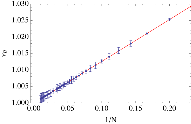
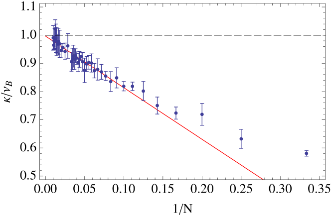
Figure 2: (Top) Collision frequency computed under equilibrium conditions with energy $E=N$ and for different system sizes $N$, ranging from $N=3$ to $N=100$, compared to the results of a numerical integration of (9) (solid red line). The $N\to\infty$ asymptotic value is 1 according to (8). The agreement is spectacular. (Bottom) RHS of equation (19), computed for the same parameters set as above. The ratio $\kappa/\nu_{\mathrm{B}}$ is the infinite $N$ limit of these data, which can be evaluated by linear regression (solid red line). Fitting all the data points corresponding to $N\geq 10$ and weighting the data according to the sizes of their error bars, we obtain $\kappa/\nu_{\mathrm{B}}=0.997\pm 0.004$.

Consider then the Helfand moment (16). We present in the bottom panel of figure 2 the results of numerical computations of equation (19), obtained for different sizes $N$ of the system, using the numerical scheme described above. As can be seen from the figure, $\lim_{n\to\infty}1/(2N)\langle\Delta H(\tau_{n})^{2}/\tau_{n}\rangle,$ has $\mathcal{O}(1/N)$ corrections to $\nu_{\mathrm{B}}$ which are due to cross-correlations of the form $\langle\eta(\epsilon_{k_{i}},\epsilon_{k_{i}+1})\eta(\epsilon_{k_{j}},\epsilon_{k_{j}+1})\rangle$ that persist for finite $N$. The infinite $N$ extrapolation of our data is obtained by linear regression and yields

$$\kappa/\nu_{\mathrm{B}}=0.997\pm 0.004\,,$$ (58)

in precise agreement with equation (23) and our argument that only static correlations contribute to the thermal conductivity.

7.2 Thermal Boundary Conditions

We simulate thermal boundary conditions according to the scheme described above, with bath relaxation frequency $\nu_{\mathrm{Bath}}=100$, fixing the baths temperatures to $T_{-}=0.5$ and $T_{+}=1.5$. The heat conductivity is then evaluated according to equation (26) by computing the average heat flux, divided by the temperature gradient, which is decreased by increasing the system size $N$. The results, displayed on the left panel of figure 3, yield the ratio

$$\kappa/\nu_{\mathrm{B}}=1.0002\pm 3\,10^{-4}\,,$$ (59)

which provides a very nice confirmation of equation (49).

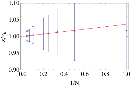
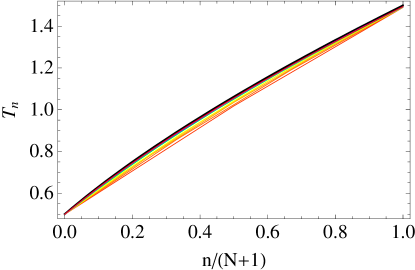
Figure 3: (Left) Ratio between the heat current (27) and local temperature gradient under thermal boundary conditions at temperatures $T_{+}=1.5$ and $T_{-}=0.5$, computed for different system sizes $N$, ranging from $N=1$ to $N=30$. The ratio $\kappa/\nu_{\mathrm{B}}$ is computed from the infinite $N$ limit of these data, evaluated by linear regression (solid red line). Fitting the data points weighed according to the sizes of their error bars, we obtain $\kappa/\nu_{\mathrm{B}}=1.0002\pm 3\,10^{-4}$. (Right) Corresponding temperature profiles with stochastically thermalised cells at $n=0$ ($T_{-}$) and $n=N+1$ ($T_{+}$). The thick black line corresponds to profile (60) expected from Fourier’s law. The data is barely distinguishable from this curve when $N$ is sufficiently large.

The corresponding temperature profiles which, according to Fourier’s law, are expected to be

$$T_{n}=\left[\frac{1}{2}(T_{-}^{3/2}+T_{+}^{3/2})+\frac{n}{N+1}(T_{+}^{3/2}-T_{-}^{3/2})\right]^{2/3}\,,$$ (60)

are shown on the right panel of figure 3.

8 Conclusions

To summarize, we have obtained a systematic derivation of Fourier’s law and computed the heat conductivity of a class of stochastic systems describing, at a mesoscopic level, the rare energy exchanges in Hamiltonian systems of two-dimensional confined particles in interaction that were introduced in [1, 2].

A remarkable feature of our approach is that the structure of the stationary state is determined by the geometry of the system and not by the actual form of the kernel which specifies the nature of the interactions between the system cells. Indeed our derivation of the two-cell distribution function only used the nearest neighbour nature of the interaction. This property alone justifies that the leading part of the distribution function, meaning including linear order in the local temperature gradients, is the local thermal equilibrium plus a two-cell function, symmetric with respect to its arguments. What precise form this function has depends on the actual process under consideration. Whatever this form, its symmetry suffices to justify that the only contributions to the heat current come from the local thermal equilibrium part, at least to the extent that the current is computed to linear order in the local temperature gradients.

We therefore conclude the same property, namely that the heat conductivity can be obtained through averages with respect to the local thermal equilibrium distributions, should hold for systems similarly described by an equation of the form (1), sustaining non-equilibrium stationary states with symmetric corrections of the form (38).

In particular, we observe that, whether or not such systems obey the gradient condition, the transport coefficient is given from the diffusion of Helfand moment, or equivalently the Green-Kubo formula, through a static average only.

Let us mention that, as observed in [10], the class of mechanical systems with confined particles in interaction that share the transport properties of the systems considered in [1, 2] is larger than the class of semi-dispersing billiards envisaged there. In particular, the systems studied in [10] do not a priori obey a master equation of the form (1). We expect that the BBGKY hierarchy applied to the phase-space distributions of these systems will have solutions with properties similar to the solutions found here, namely a local thermal equilibrium part plus a symmetric correction which does not contribute to the heat current.

References

References

- [1] Gaspard G and Gilbert T 2008 Heat conduction and Fourier’s law by consecutive local mixing and thermalization Phys Rev Lett 101 020601
- [2] Gaspard G and Gilbert T 2008 Heat conduction and Fourier’s law in a class of many particle dispersing billiards New J Phys in press; arXiv:0802.4455
- [3] Uhlenbeck G E The Boltzmann equation in Kac M 1959 Probability and related topics in physical sciences Lectures in Applied Mathematics 1 (Interscience, New York)
- [4] Van Kampen N G 2000 Views of a Physicist: Selected Papers Meijer P H E ed. (World Scientific, Singapore)
- [5] Spohn H 1991 Large Scale Dynamics of Interacting Particles (Springer-Verlag, Berlin)
- [6] Gillespie D T 1976 General Method for Numerically Simulating the Stochastic Time Evolution of Coupled Chemical Reactions J Comp Phys 22 403-434
- [7] Gillespie D T 1977 Exact Stochastic Simulation of Coupled Chemical Reactions J Phys Chem 81 2340-2361
- [8] Helfand E 1960 Transport Coefficients from Dissipation in a Canonical Ensemble Phys Rev 119 1
- [9] Press W H, Flannery B P, Teukolsky S A, and Vetterling W T 1992 Numerical Recipes in Fortran, 2nd ed. (Cambridge University Press, Cambridge, England)
- [10] Gilbert T and Lefevere R 2008 Heat conductivity from molecular chaos hypothesis in locally confined billiard systems Phys. Rev. Lett. in press; arXiv:0808.1179