Abstract

A current problem of practical significance is the analysis of large, spatially distributed, environmental data sets. The problem is more challenging for variables that follow non-Gaussian distributions. We show by means of numerical simulations that the spatial correlations between variables can be captured by interactions between “spins”. The spins represent multilevel discretizations of environmental variables with respect to a number of pre-defined thresholds. The spatial dependence between the “spins” is imposed by means of short-range interactions. We present two approaches, inspired by the Ising and Potts models, that generate conditional simulations of spatially distributed variables from samples with missing data. Currently, the sampling and simulation points are assumed to be at the nodes of a regular grid. The conditional simulations of the “spin system” are forced to respect locally the sample values and the system statistics globally. The second constraint is enforced by minimizing a cost function representing the deviation between normalized correlation energies of the simulated and the sample distributions. In the approach based on the $N_{c}-$state Potts model, each point is assigned to one of $N_{c}$ classes. The interactions involve all the points simultaneously. In the Ising model approach, a sequential simulation scheme is used: the discretization at each simulation level is binomial (i.e., $\pm 1$.) Information propagates from lower to higher levels as the simulation proceeds. We compare the two approaches in terms of their ability to reproduce the target statistics (e.g., the histogram and the variogram of the sample distribution), to predict data at unsampled locations, as well as in terms of their computational complexity. The comparison is based on a non-Gaussian data set (derived from a digital elevation model of the Walker lake area, Nevada, USA). We discuss the impact of relevant simulation parameters, such as the domain size, the number of discretization levels, and the initial conditions.

[Multilevel Discretized Random Fields and Spatial Simulations] Multilevel Discretized Random Field Models with “Spin” Correlations for the Simulation of Environmental Spatial Data Milan Žukovič Dionissios T. Hristopulos Keywords: New applications of statistical mechanics, Analysis of algorithms

1 Introduction

Spatially distributed data are common in the physical sciences. They represent various environmental variables, such as contaminant concentrations in the atmosphere, soil permeability and dispersivity, etc. To account for the spatial variation and the measurement uncertainty of such quantities, the mathematical model of spatial random fields is commonly used. To date, huge numbers of large spatial data sets are gathered from around the globe on a daily basis. The efficient storage, analysis, harmonization, and integration of such data is of great importance in various scientific areas such as image processing, pattern recognition, remote sensing, and environmental monitoring. Often the data coverage is incomplete for various reasons, such as meteorological conditions (measurements hindered by clouds, aerosols, or heavy precipitation) or equipment limitations (values below detection level or resolution threshold). Hence, in order to use standard tools for the data analysis and visualization, one needs to deal with the problem of incomplete (missing) data. In addition, data sampled at different resolutions may need to be combined (e.g., in data fusion methods). This requires down-scaling (refining) of the data with the coarser resolution.

These tasks can be performed by means of well established interpolation and classification techniques [1]. While deterministic methods (e.g., nearest-neighbor or inverse distance interpolation) can be used, stochastic methods are often preferred because they are more flexible in incorporating spatial correlations and and they provide estimates of prediction uncertainty. However, considering the ever-increasing size of spatial data, stochastic methods such as kriging [2], can be impractical due to their high computational complexity, requiring the use of high performance computational technologies [3]. Furthermore, kriging is founded on the assumption of a jointly Gaussian distribution, which is often failed by the data. Practical application of kriging involves considerable human (subjective) input, regarding the selection of the correlation (variogram) model and the kriging neighborhood selection [4].

The classical geostatistical approach relies on the structure function (variogram) for modeling the spatial correlations. However, the correlations can also be considered as the outcome of “interactions” between the field values at different points [5] that generate short-range spatial order. In the case of static disorder, which is typical in case of “quenched” geological disorder or measurements representing a single time slice of a dynamical process, such interactions represent “effective constraints” imposed by the underlying process. For example, in the case of a digital elevation model, these constraints are imposed by the topography of the area. While the nature of the constraints may differ significantly between processes, we believe that universal aspects of spatial correlations can be captured by means of relatively simple effective interactions. By incorporating the interactions in an energy functional a Gibbs probability measure can be defined as in [5]. The realization probability of each spatial configuration is then governed by the relative weight of the “many body” Gibbs probability density function. In the Gaussian case it is straightforward to define the interactions between the random field values at neighboring locations. On a regular lattice this approach defines Gauss-Markov random fields.

In the non-Gaussian case, it is convenient to discretize the continuous values of the random field using a set of discrete “spins”. We arbitrarily define higher spin values to represent higher values of the field. In the spirit described above, one can then consider interactions between different “spins”. In this framework, the problems of spatial interpolation and simulation are mapped into a spatial classification problem, in which each “prediction” location is assigned to a specific spin value (class). The concept of classical spins is a suitable choice for modeling the multilevel discretization of the continuous field. Spin models from statistical physics, e.g., the Ising and Potts models, have already been applied in various problems in economy and finance [6, 7, 8], materials science [9, 10, 11], and biology [12]. However, these studies focus mainly on long-range correlations. In the framework of Gibbs-Markov random fields, the short-range correlation properties of Potts and Ising models have been widely applied in image analysis (see e.g. [13, 14, 15, 16, 17]). The Potts model in super-paramagnetic regime was also proposed as a data clustering model [18]. We introduce here two non-parametric models for spatial classification that are loosely based on the Ising and Potts spin models. The first model employs a sequential classification approach while the second a simultaneous (parallel) classification of all levels.

The rest of the paper is organized as follows. In Section 2, we present the problem of spatial classification/prediction, and we review the commonly used classification algorithm of $k$-nearest neighbors. Section 3 briefly reviews the Ising and Potts models and introduces the “spin” nearest-neighbor correlation models that we propose for spatial classification. In Section 4 we investigate technical aspects of the simulations, and we describe computational details. Section 5 focuses on the case study: it presents computational details as well as the analysis of the simulation results. Finally, in Section 6, we summarize the relevant results and point out some future directions.

2 Spatial prediction and classification

Let us consider a set of sampling points $G_{s}=\{\vec{r}_{i}\}$, where $\vec{r}_{i}=(x_{i},y_{i})\in{\mathbb{R}}^{2}$ and $i=1,\ldots,N$. These points are assumed to be scattered on a rectangular grid $\tilde{G}$ of size $N_{\tilde{G}}=L_{x}\,L_{y}>N$, where $L_{x}$ and $L_{y}$ are respectively the number of nodes in the orthogonal directions (in terms of the unit length). If $z_{i}$ is a value attributed to the point $\vec{r}_{i}$, the set $Z\{G_{s}\}=\{z_{i}\in{\mathbb{R}}\}$ represents the sample of the process. Here we assume that $Z\{G_{s}\}$ represents a sample from a realization of a continuous random field ${\rm Z}({\vec{r}};\omega),$ where $\omega$ is the state index.

Let $G_{p}=\{\vec{r}_{p}\}$ be the set of prediction points where $p=1,\ldots,P$, such that $\tilde{G}=G_{s}\cup G_{p}$. We discretize the continuous distribution of $Z$ using a number of classes, ${\mathcal{C}}_{q},\,q=1,\ldots,N_{c}$. The classes are defined with respect to a set of threshold levels $t_{k},\,k=1,\ldots,N_{c}+1$. If $z_{\min}=\min(z_{1},\ldots,z_{N})$, $z_{\max}=\max(z_{1},\ldots,z_{N}),$ $\delta t=(z_{\max}-z_{\min})/N_{c}$, the thresholds are defined as: $t_{1}=-\infty$, $t_{2}=z_{\min}+\delta t$, $t_{i}=t_{i-1}+\delta t$ $(i=3,\ldots,N_{c})$ and $t_{N_{c}+1}=\infty$. Each class ${\mathcal{C}}_{q}$ corresponds to the interval ${\mathcal{C}}_{q}=(t_{q},t_{q+1}]$ for $q=1,\ldots,N_{c}$. This means that all the classes, except the first and the last, have a uniform width. The classes ${\mathcal{C}}_{1}$ and ${\mathcal{C}}_{N_{c}}$ extend to infinity (negative and positive respectively), to allow for values at the prediction points that lie outside the observed interval $[z_{\min},z_{\max}]$. We define the class indicator field (phase field) $I_{Z}(\vec{r})$ by means of

$$I_{Z}(\vec{r}_{i})=\sum_{q=1}^{N_{c}}q\,\left[\theta\left(z_{i}-t_{q}\right)-\theta\left(z_{i}-t_{q+1}\right)\right],\quad\forall i=1,\ldots,N,$$ (1)

where $\theta(x)=1$ for $x>0$ and $\theta(x)=0$ for $x\leq 0$ is the unit step function. Prediction of the field values $Z\{G_{p}\}$ is mapped onto a classification problem, i.e., into estimating $\hat{I}_{Z}\{G_{p}\}$. If the number of levels is high, the continuum limit is approached.

2.1 $k$-nearest neighbor ($k$-NN) classifier

The $k$-NN method is a supervised learning algorithm, which assigns to each prediction point the class represented by the majority of its $k$ nearest neighbors from the sample [19]. The distance metric used is typically Euclidean. The optimal value of the parameter $k$ depends on the data and requires tuning for different applications. The optimization of $k$ usually involves heuristic techniques (e.g. cross-validation). The accuracy of the $k$-NN classifier is affected by noise or by selecting a neighborhood that does not include the pertinent spatial information. The $k$-NN algorithm has been widely applied in the field of data mining, statistical pattern recognition, image processing and many others. In general, it has been found to outperform many other flexible nonlinear methods, particularly in high-dimensional spaces [20]. Furthermore, it is relatively easy to implement and has desirable consistency properties, e.g., favorable asymptotic classification error dependence.

We use the $k$-NN classifier as a benchmark for the “spin-based” classification methods we propose. To eliminate the effect of $k$ on the classification results, for each simulated realization we perform the classification for a wide range of values of $k=1,\ldots,k_{\max}$, and select the value $k_{\rm opt}$ that minimizes the misclassification rate.

3 Spatial Classification based on “spin” correlation models

We propose two non-parametric, nearest-neighbor (NN), multilevel correlation (MLC) models that are loosely based on the Ising and Potts models. The NN-MLC models are based on matching suitably normalized correlation energy functions calculated from the samples with those estimated over the entire prediction grid. Similar ideas of correlation energy matching were also applied in the reconstruction of digitized random media from limited morphological information [21, 22]. In contrast with those studies, in the NN-MLC models we also use local spatial information (i.e., the values at the sampling points). The prediction of the field values (more precisely, class) at unsampled locations is achieved by means of conditional simulations that respect locally the sample values and the correlation energy globally.

3.1 Ising model

The Ising model (e.g. [23]) involves discrete variables $s_{i}$ (spins) placed on a sampling grid. Each spin can take two values, $\pm 1$, and the spins interact in pairs. Assuming only nearest-neighbor interactions, the energy of the system can be expressed by the following Hamiltonian:

$$H_{I}=-\sum_{i,j}J_{ij}s_{i}s_{j}-\sum_{i}h_{i}s_{i}.$$

The coupling strength $J_{ij}$ controls the type (ferromagnetic for $J_{ij}>0$, antiferromagnetic for $J_{ij}<0$) and strength of the interactions. The second term introduces a symmetry-breaking bias caused by the presence of a site dependent external field $h_{i}$. The latter controls the mean spin value (the magnetization). The model is usually defined on a regular grid, the interactions are considered uniform and their range limited to nearest neighbors. However, the model can be generalized to include also irregular grids and longer-range interactions.

3.2 Potts model

The Potts model is a generalization of the Ising model (e.g. [24]). Instead of $\pm 1$, each spin is assigned an integer value $s_{i}\in\{1,\ldots,N_{c}\}$, where $N_{c}$ represents the total number of states or classes. The Hamiltonian of the Potts model is given by

$$H_{P}=-\sum_{i,j}J_{ij}\delta_{(s_{i},s_{j})}-\sum_{i}h_{i}s_{i},$$

where $\delta$ is the Kronecker delta. Hence, only pairs of spins in the same state give a non-zero contribution to the correlation energy. For $N_{c}=2$, the Potts model is equivalent to the 2D Ising model.

3.3 General Assumptions for NN-MLC Classifiers

The states (configurations) of both the Ising and Potts models are determined by the Gibbs probability density function $f=Z^{-1}\,\exp(-H/k_{B}T),$ where $H$ is the respective Hamiltonian, $k_{B}$ is the Boltzmann’s constant, and $T$ is the temperature. The partition function $Z$ is obtained by summing $e^{-H/k_{B}T}$ over all possible spin configurations. Essentially, the Hamiltonian involves two parameters, i.e. the normalized interaction couplings $\tilde{J}_{ij}=J_{ij}/k_{B}T$ and $\tilde{h}_{i}=h_{i}/k_{B}T.$ In the case of spatial classification, the parameters are not known a priori and need to be determined from the sample. The standard procedure for this inverse problem entails using the maximum likelihood method. Assuming that the parameters can be inferred, the spin values at unsampled locations are predicted by maximizing the conditional probability density function $f\left(I_{Z}\{G_{p}\}|I_{Z}\{G_{s}\};\tilde{J}_{ij},\tilde{h}_{i}\right)$. However, optimizing the likelihood of the models with respect to the coupling parameters $\tilde{J}_{ij},\tilde{h}_{i}$ is a computationally intensive task, since there are no generally valid closed-form expressions for the partition function. In order to overcome this problem we opted for a non-parametric approach.

Our NN-MLC models retain only the interaction energies of the Ising and Potts spin Hamiltonians. The sample values $Z\{G_{s}\}$ are mapped into spin values by suitable discretization (as shown below). The main idea in both methods is to match the sample correlation energy with the correlation energy of all the spins (i.e. including the simulated spins at prediction points). This relies on the ergodic assumption that the sample spin correlation energies accurately describe those of the entire system. The matching of the correlation energies is performed by means of a numerical Monte Carlo approach. During the process, the spins at the sample sites remain fixed. Hence, the procedure followed is conditional simulation, as opposed to deterministic prediction. Focusing on regular grids and assuming isotropic and nearest-neighbor “spin interactions,” it is reasonable to set $J_{ij}=J_{0}$ if the points $\vec{r}_{i}$, $\vec{r}_{j}$ are lattice neighbors and $J_{ij}=0$ otherwise. Furthermore, we set $h_{i}=0\,(i=1,\ldots,N)$. This choice prevents explicit control of the mean spin. Nevertheless, as shown by the simulation results, judicious choice of the initial state allows the distribution of the predicted classes to accurately recover the class distribution of the sample. This is due to the fact that both the correlation energies and the local spin values are restricted by the sample.

3.4 Ising-based NN-MLC model (I-NN-MLC)

We propose a sequential scheme in which the sample, $G_{s}^{q}$ and prediction, $G_{p}^{q}$ grids are sequentially updated. Each simulation level $q$ corresponds to a class index. The number of simulation levels coincides with that of discretization levels. For the lowest level $G_{s}^{1}=G_{s},\,G_{p}^{1}=G_{p}.$ For $q=1,\ldots,N_{c}-1$ it holds that $G_{s}^{q}\subseteq G_{s}^{q+1}$, $G_{p}^{q}\supseteq G_{p}^{q+1}$ and $\tilde{G}=G_{s}^{q}\cup G_{p}^{q}.$ Binary-valued spins are used at each level $q(q=1,\ldots,N_{c})$. Sites (either from the sample or simulated) having $I_{Z}\leq q$ are assigned a spin value of $-1,$ while sites having $I_{Z}>q$ are assigned a spin value of $1$. All the sites that are assigned a spin $-1$ value at level $q$ retain this value at higher levels. This means that the areas of low values are classified first. Once a site $\vec{r}_{i}$ is assigned a spin $-1$ value at level $q<N_{c}$, it is also assigned class value $I_{Z}(\vec{r}_{i})=q.$ At the same time, the set $G_{s}^{q+1}$ acquires all the $-1$ points while the set $G_{p}^{q+1}$ is accordingly reduced. In contrast, for sites that are assigned spin $1$ value $I_{Z}(\vec{r}_{i})>q$, and the precise class value $I_{Z}(\vec{r}_{i})$ is determined at a higher level. At level $q=N_{c}$ all remaining sites are assigned to the $N_{c}$-th class.

Let $S^{q}_{s}=\{s_{i}^{q};\,\forall\,i\,\mbox{s.t.}\,\vec{r}_{i}\in G_{s}^{q}\}$, $\forall q=1,\ldots,N_{c},$ be the set of spin values included in the “sample” at level $q$. These values are $\pm 1$ (depending on $z_{i}$) if $\vec{r}_{i}\in G_{s}$ and $-1$ if $\vec{r}_{i}$ is an already classified prediction point. The unknown values at level $q$ are the spins at the remaining locations, denoted by $S^{q}_{p}$.

Our non-parametric approach utilizes a cost function, $U_{\rm I}(S^{q}_{p}|S^{q}_{s}),$ that describes the deviation between the normalized correlation energies of the simulated spin configuration, $\tilde{C}_{\rm I}^{q}$, and its sample counterpart, $C_{{\rm I};s}^{q}$ estimated from the spins in $G_{s}^{q}$.

$$U_{\rm I}(S^{q}_{p}|S^{q}_{s})=\left\{\begin{array}[]{ll}\Big{[}1-\tilde{C}^{q}_{\rm I}(S^{q}_{p},S^{q}_{s})/C_{{\rm I};s}^{q}(S^{q}_{s})\Big{]}^{2},&{\rm{for}}\ C_{{\rm I};s}^{q}\neq 0,\\ \\ \tilde{C}^{q}_{\rm I}(S^{q}_{p},S^{q}_{s})^{2},&{\rm{for}}\ C_{{\rm I};s}^{q}=0,\end{array}\right.$$ (5)

where $C_{{\rm I};s}^{q}(S^{q}_{s})=\langle s^{q}_{i}\,s^{q}_{j}\rangle_{G_{s}^{q}}$ is the spatially averaged (normalized by the number of nearest neighbor pairs in $G_{s}^{q}$) spin pair correlation of the $q-$level sample and $\tilde{C}^{q}_{\rm I}(S^{q}_{p},S^{q}_{s})=\langle s^{q}_{i}s^{q}_{j}\rangle_{\tilde{G}}$ is the spatially averaged spin pair correlation over the entire grid. Given the above, the estimation of $S^{q}_{p}$ is equivalent to finding the optimal configuration $\hat{S}^{q}_{p}$ that corresponds to the minimum of the cost function (5) at a fixed temperature $T$, i.e.,

$$\hat{S}^{q}_{p}={\rm arg\,min}_{S^{q}_{p}}\,U_{\rm I}(S^{q}_{p}|S^{q}_{s}),\,\mbox{for}\;q=1,\ldots,N_{c}.$$ (6)

3.5 Potts-based NN-MLC model (P-NN-MLC)

In the P-NN-MLC model the classification is performed for all classes simultaneously. Hence, there is only a single simulation level irrespectively of the number of discretization levels. The grid spins $S=\{s_{i}\}$, $i=1,\ldots,N$ take values in the set $s_{i}\in\{1,\ldots,N_{c}\}$. The cost function is given by

$$U_{\rm P}(S_{p}|S_{s})=\left\{\begin{array}[]{ll}\Big{[}1-\tilde{C}_{\rm P}(S_{p},S_{s})/C_{{\rm P};s}(S_{s})\Big{]}^{2},&{\rm{for}}\ C_{{\rm P};s}\neq 0,\\ \\ \tilde{C}_{\rm P}(S_{p},S_{s})^{2},&{\rm{for}}\ C_{{\rm P};s}=0,\end{array}\right.$$ (10)

where $C_{{\rm P};s}(S_{s})=\langle\delta_{(s_{i},s_{j})}\rangle_{G_{s}}$ is the spatially averaged (normalized by the number of nearest neighbor pairs in $G_{s}$) spin pair correlation of the sample and $\tilde{C}_{\rm P}(S_{p},S_{s})=\langle\delta_{(s_{i},s_{j})}\rangle_{\tilde{G}}$ is the average spin pair correlation over ${\tilde{G}}$. The estimation of $S_{p}$ is equivalent to finding the minimum of the cost function (10), i.e.,

$$\hat{S}_{p}={\rm arg\,min}_{S_{p}}\,U_{\rm P}(S_{p}|S_{s}).$$ (11)

4 Simulations of Missing Data on Regular Grids

We focus on samples with missing data on regular grids. On such grids, it is straightforward to determine the nearest neighbors and calculate the correlation energies. Both the I-NN-MLC and P-NN-MLC methods return a class indicator field [see Eq. (1)] $\hat{I}_{Z}=I_{Z}(G_{s})\cup\hat{I}_{Z}(G_{p})$, which consists of the original sample classification and the class estimates at $G_{p}$. The indicator values at the sampling sites are exactly reproduced. Below we refer to $I_{Z}(G_{s})$ as the training set. Optimization of the cost functions (5) and (10) are performed using the Monte Carlo approach. The generation of new “trial” spin states is realized using the Metropolis algorithm at zero temperature.

We use the rejection ratio defined by $\rho=(\#\mbox{rejected states})/N(G_{p}^{q}),$ where $N(G_{p}^{q})$ is the number of prediction points at the $q$-level, to determine the stopping criterion. More specifically, our simulations terminate if $\rho=1$, i.e., if one complete sweep through the entire grid $G_{p}^{q}$ does not produce a single successful update. Reaching the termination criterion may require several sweeps through the lattice, depending on the initial state.

4.1 Greedy Monte Carlo

The $T=0$ assumption implies that the stochastic selection of an energetically unfavorable spin configuration in the Metropolis step is not possible. Hence, the candidate “spin” for the update is flipped unconditionally only if it lowers the cost function. This approach is called the “greedy” Monte Carlo algorithm [25] and leads to very fast convergence. In contrast, in simulated annealing $T$ is slowly lowered starting from an initial high-temperature state. This approach is much slower computationally. However, the configuration resulting from simulated annealing is less sensitive to the initial state. The sensitivity of the greedy algorithm is known to be especially pronounced in high-dimensional spaces with non-convex energies. In such cases, the greedy algorithm is likely to be trapped in local minima, instead of converging to the global one. However, this is not a concern in the current problem. In fact, targeting the global minimum of $U_{\rm I}$ and $U_{\rm P}$ strongly emphasizes the sample correlation energy per “spin” pair. However, the latter is influenced by sample-to-sample fluctuations.

On rectangular or square grids, further increase in computational efficiency is gained by taking advantage of the geometry and the nearest-neighbor interactions. This is achieved by splitting the grid into two interpenetrating subgrids, which allows vectorizing the algorithm. Hence, one sweep through the entire grid is performed in just two steps by simultaneously updating all the sites on one of the subgrids in each step.

4.2 Simulation Algorithms

Based on the above, the monte Carlo (MC) algorithms for the I-NN-MLC and P-NN-MLC models consist of the following steps:

Algorithm for I-NN-MLC model

(1) Initialize the indicator field on the entire grid by means of $\hat{I}_{Z}(\tilde{G})={\rm NaN}$
(2) Set the simulation level (class index) to $q=1$
(3) While [loop 1] $q\leq N_{c}-1$ discretize $Z\{G_{s}\}$ with respect to $t_{q+1}$ to obtain $S^{q}_{s}$
(3.1) Given the data $S^{q}_{s}$, calculate the sample correlation energy $C_{I;s}^{q}$
(3.2) Assign initial values to the spins at $G^{q}_{p},$ i.e., generate $\hat{S}^{q\,(0)}_{p}$
(3.3) Calculate the initial values of the simulated correlation $\tilde{C}_{I}^{q\,(0)}$
and the cost function $U_{I}^{(0)}$; initialize the MC index $i=1$
(3.4) Initialize the rejection ratio $\rho\rightarrow 0;$ and the rejected states index $i_{r}=0$
(3.5) While [loop 2] $\rho<1$ repeat the following updating steps:
(3.5.1)Generate a new state $\hat{S}^{q\,(i+1)}_{p}$ by perturbing $\hat{S}^{q\,(i)}_{p}$
(3.5.2)Calculate $\tilde{C}_{I}^{q\,(i+1)}$ and $U_{I}^{(i+1)}$
(3.5.3) If $U_{I}^{(i+1)}<U_{I}^{(i)}$ accept the new state; $i_{r}\rightarrow 0.$
else keep the “old” state; $i_{r}\rightarrow i_{r}+1$; endif
(3.5.4) $\rho\rightarrow i_{r}/N(G_{p}^{q});\,i\rightarrow i+1$;
end [loop 2]
(3.6) Assign the $-1$ “spins” to the $q$ level, i.e., $\hat{I}_{Z}(\{\vec{r}_{i}\})=q$
If $\hat{S}^{(i_{\max})}(\{\vec{r}_{i}\})=-1$, $\{\vec{r}_{i}\}\in\tilde{G}$
(3.7) Increase simulation level, $q\rightarrow q+1$, return to step (3)
end [loop 1]
(4) For $q=N_{c}$, $\forall\vec{r}_{i}\;(i=1,\ldots,N_{\tilde{G}})$ such that $\hat{I}_{Z}(\{\vec{r}_{i}\})={\rm NaN}$, set $\hat{I}_{Z}(\{\vec{r}_{i}\})=N_{c}\;$.

In the above, the symbol NaN is used to denote non-numeric values.

Algorithm for P-NN-MLC model

(1) Discretize $Z\{G_{s}\}$ with respect to $t_{k},\ k=1,\ldots,N_{c}+1$ to obtain $S_{s}$
(2) Given the data $S_{s}$, calculate the sample correlation energy $C_{P;s}$
(3) Assign initial values to the spins at $G_{p},$ i.e., generate $\hat{S}^{(0)}_{p}$
(4) Calculate the initial values of the simulated correlation $\tilde{C}_{P}^{(0)}$
and the cost function $U_{P}^{(0)}$; initialize the MC index $i=1$
(5) Initialize the rejection ratio $\rho\rightarrow 0;$ and the rejected states index $i_{r}=0$
(6) While $\rho<1$ repeat the following updating steps:
(6.1) Generate a new state $\hat{S}^{(i+1)}_{p}$ by perturbing $\hat{S}^{(i)}_{p}$
(6.2) Calculate $\tilde{C}_{P}^{(i+1)}$ and $U_{P}^{(i+1)}$
(6.3) If $U_{P}^{(i+1)}<U_{P}^{(i)}$ accept the new state; $i_{r}\rightarrow 0.$
else keep the “old” state; $i_{r}\rightarrow i_{r}+1$; endif
(6.4) $\rho\rightarrow i_{r}/N(G_{p});\,i\rightarrow i+1$;
end
(7) Assign $\hat{I}_{Z}(\{\vec{r}_{i}\})=\hat{S}^{(i_{\max})}(\{\vec{r}_{i}\})$, $\{\vec{r}_{i}\}\in\tilde{G}$.

4.3 Initial state selection

The initial configuration of class indices can be selected in a number of ways. Since the proposed models aim to provide fast and automatic classification mechanisms, the initial configuration (assigned in steps (3.2) and (3) in the I-NN-MLC and P-NN-MLC algorithms) should minimize the relaxation path in state space to the equilibrium. It should also be selected with little or no user intervention. Since a degree of spatial continuity is common in geospatial data sets, it makes sense that the initial state of the individual prediction points is determined based on the sample states in their immediate neighborhood. On square grids, we determine the neighborhood of ${\vec{r}_{p}}$ by an $m\times m$ stencil (where $m=2l+1$) centered at ${\vec{r}_{p}}$. Then, the initial value at a prediction point is assigned by majority rule, based on the prevailing value of its sample neighbors inside the stencil. If we considered a circular stencil, this method would correspond to the $k$-NN classification algorithm, $k$ being the number of sampling points inside the stencil.

We set the stencil size adaptively to the smallest size that contains a clear majority of sample spin values, as shown schematically in Fig. (1). In practice, it makes sense to impose an upper limit on the stencil size $m_{\max}$. If no majority is established up to the maximum stencil size $m_{\max}\times m_{\max}$, the initial value at ${\vec{r}_{p}}$ is assigned randomly from the equally represented class indices with the highest frequency (in the I-NN-MLC this means $\pm 1.$) If majority is not reached due to absence of sampling points inside the maximum stencil, the initial value is drawn randomly from the entire range of the labels $1,\ldots,N_{c}$. There are sensible reasons for imposing a maximum stencil size. First, considering too large neighborhoods in the $k$-NN classification generally generates oversmoothing at larger-scales that can not be justified as an effect of local continuity. Second, large neighborhoods increase the computational demands (both for memory and CPU time) disproportionately to expected benefits. Finally, assigning a portion of the prediction points initial values at random introduces a degree of randomness, which can be used to assess uncertainty by performing multiple runs on the same sample set. The choice of $m_{\max}$ is arbitrary to an extent. Intuitively, for sparser sampling patterns larger $m_{\max}$ should be considered. In our investigations, relatively small sizes (up to $m_{\max}=7$) were sufficient to establish good statistical performance at relatively small computational cost.

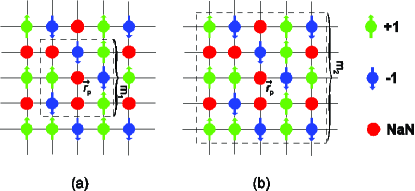
Figure 1: Schematic demonstrating the stencil selection. Arrows pointing up correspond to $+1$ spins, arrows pointing down to $-1$ spins, and the empty circles to the prediction location. In the first plot (a) a square stencil of size $m_{1}$=3 is used. Within the neighborhood marked by the dash-line square there is an equal number of $+1$ and $-1$ sites. In the second plot (b) a stencil of size $m_{2}=5$ is used to break the tie.

The algorithms thus require that only two parameters be set: $m_{\max}$ and $N_{c}$. The latter depends on the study’s objectives: if the goal is to determine exceedance levels of a pollutant concentration with respect to a regulatory threshold, a binary classification is adequate. For environmental monitoring and decision making purposes a moderate number of classes (e.g., eight) is often sufficient.

5 Case Study: Missing Data Reconstruction

To test the classification models we use a synthetic pollutant concentration data set derived from a digital elevation model of the Walker lake area in Nevada [26]. A two-dimensional projection of the pollution field is shown in Fig. 2(a). The units used for the $Z$ values are arbitrarily set to parts per million (ppm). Some summary statistics are as follows: number $N_{\tilde{G}}=78\ 000$ on a $260\times 300$ rectangular grid, $z_{\min}=0$, $z_{\max}=1631.2$, $\bar{z}=277.9$, $z_{0.50}=221.3$, $\sigma_{z}=249.9$, the skewness coefficient is $1.02$, and the kurtosis coefficient $3.78$. As evidenced from the above statistics and the histogram in Fig. 2(b), the distribution is clearly neither Gaussian nor log-normal.

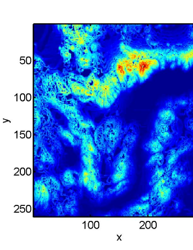
(a) Map

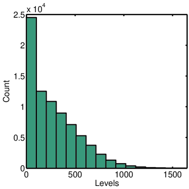
(b) Histogram

Figure 2: Map and histogram of the original complete data.

5.1 Computational details

¿From the complete data we draw a sample $Z\{G_{s}\}$ (training set) of size $N=(1-p)N_{\tilde{G}}$ by randomly removing $P=pN_{\tilde{G}}$ values (validation set), which are later used for prediction validation. For three degrees of thinning, $p=[0.33,0.50,0.66]$, we generate $100$ different configurations of the training and validation sets. The values at the prediction points are predicted (classified) using the I-NN-MLC and P-NN-MLC classification algorithms. The class indicator values at the prediction points $I_{Z}(G_{p})$ are then compared with the classification estimates $\hat{I}_{Z}(G_{p})$. To evaluate the classification performance, we calculate the misclassification rate as a fraction of misclassified pixels:

$$F=\frac{1}{P}\sum_{p=1}^{P}\left[1-\delta\big{(}I_{Z}(\vec{r}_{p}),\hat{I}_{Z}(\vec{r}_{p})\big{)}\right],$$ (12)

where $I_{Z}(\vec{r}_{p})$ is the true value at the validation points, $\hat{I}_{Z}(\vec{r}_{p})$ is the classification estimate and $\delta(I,I^{\prime})=1$ if $I=I^{\prime}$, $\delta(I,I^{\prime})=0$ if $I\neq I^{\prime}$. The standard deviation of the quantity $F$ is evaluated using the values obtained from all the configurations, as ${\rm STD}_{F}=\sqrt{\sum_{i=1}^{100}(F_{i}^{*}-\overline{F_{i}^{*}})^{2}/99}$. We also compare the class index variograms of the original and reconstructed patterns in the orthogonal lattice directions, defined by

$$\hat{\gamma}_{\iota}(h)=\frac{1}{2|N_{\iota}(h)|}\sum_{i,j\in N_{\iota}(h)}|I_{Z}(\vec{r}_{i})-I_{Z}(\vec{r}_{j})|^{2},$$ (13)

where $N_{\iota}(h)$ denotes the set of pairs of points in $\iota$ orthogonal lattice direction separated by distance $h$ (lag), and $|N_{\iota}(h)|$ denotes the number of pairs in the set.

Furthermore, we record the CPU time, the number of MC sweeps needed to reach equilibrium, and the residual values of the cost functions at termination. The procedure is repeated for $N_{c}=8$ and $N_{c}=16$. The computations are performed in the Matlab® programming environment on a desktop computer with 1.93 GB of RAM and an Intel®Core™2 CPU 6320 processor at 1.86 GHz.

(a) I-NN-MLC, $p=0.33$

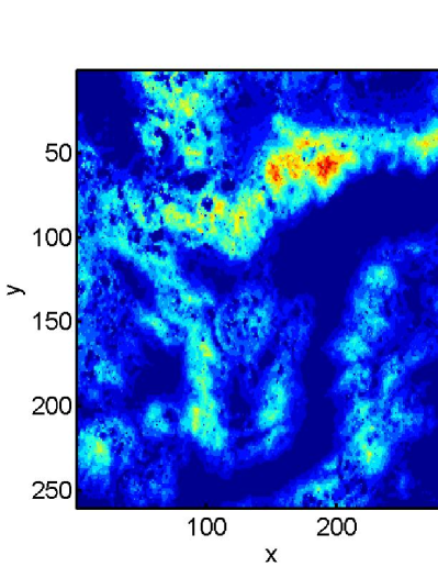
(b) I-NN-MLC, $p=0.66$

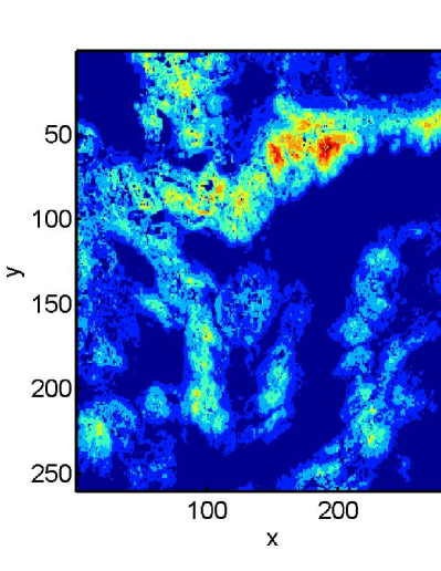
(c) P-NN-MLC, $p=0.33$

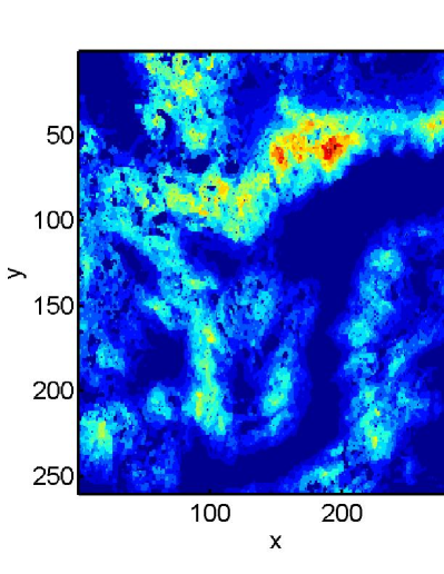
(d) P-NN-MLC, $p=0.66$

Figure 3: The reconstructed maps corresponding to the first realization obtained by (a) I-NN-MLC with $p=0.33$, (b) I-NN-MLC with $p=0.66$, (c) P-NN-MLC with $p=0.33$, and (d) P-NN-MLC with $p=0.66$.

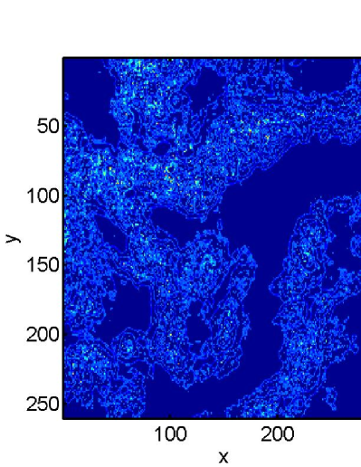
(a) I-NN-MLC, $p=0.33$

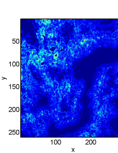
(b) I-NN-MLC, $p=0.66$

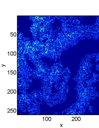
(c) P-NN-MLC, $p=0.33$

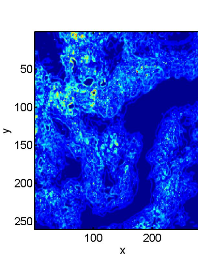
(d) P-NN-MLC, $p=0.66$

Figure 4: The standard deviations calculated based on the classification results obtained from $100$ realizations obtained by (a) I-NN-MLC with $p=0.33$, (b) I-NN-MLC with $p=0.66$, (c) P-NN-MLC with $p=0.33$, and (d) P-NN-MLC with $p=0.66$.

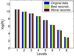
(a) I-NN-MLC, $p=0.33$

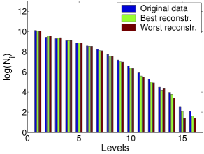
(b) I-NN-MLC, $p=0.66$

(c) P-NN-MLC, $p=0.33$

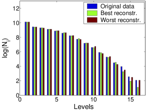
(d) P-NN-MLC, $p=0.66$

Figure 5: The log-histograms of the original, the best $(F^{*}_{min}),$ and the worst $(F^{*}_{max})$ reconstructed data, obtained by (a) I-NN-MLC with $p=0.33$, (b) I-NN-MLC with $p=0.66$, (c) P-NN-MLC with $p=0.33$, and (d) P-NN-MLC with $p=0.66$.

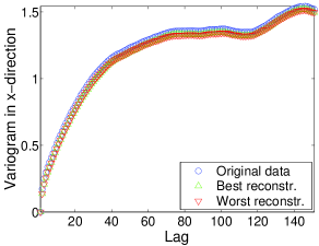
(a) I-NN-MLC, $p=0.33$

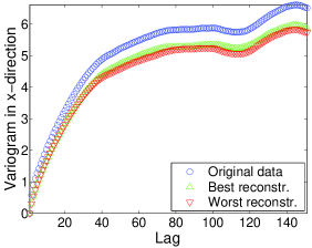
(b) I-NN-MLC, $p=0.66$

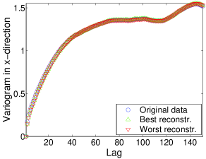
(c) P-NN-MLC, $p=0.33$

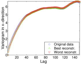
(d) P-NN-MLC, $p=0.66$

Figure 6: The x-axis direction variograms of the original, the best $(F^{*}_{min}),$ and the worst $(F^{*}_{max})$ reconstructed data, obtained by (a) I-NN-MLC with $p=0.33$, (b) I-NN-MLC with $p=0.66$, (c) P-NN-MLC with $p=0.33$, and (d) P-NN-MLC with $p=0.66$.

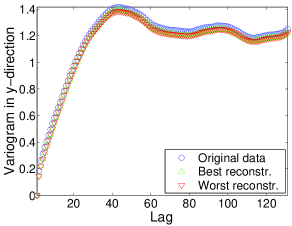
(a) I-NN-MLC, $p=0.33$

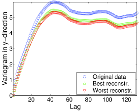
(b) I-NN-MLC, $p=0.66$

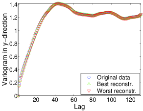
(c) P-NN-MLC, $p=0.33$

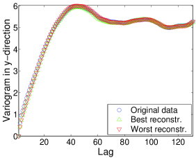
(d) P-NN-MLC, $p=0.66$

Figure 7: The y-axis direction variograms of the original, the best $(F^{*}_{min}),$ and the worst $(F^{*}_{max})$ reconstructed data, obtained by (a) I-NN-MLC with $p=0.33$, (b) I-NN-MLC with $p=0.66$, (c) P-NN-MLC with $p=0.33$, and (d) P-NN-MLC with $p=0.66$.

5.2 Analysis of Missing Data Reconstruction Results

In Figs. 3 - 7 the classification performance of the two spin-based models is demonstrated for two limiting cases: one with a low number of levels and low degree of thinning ($N_{c}=8$ and $p=0.33$), and the other one with a high number of levels and high degree of thinning ($N_{c}=16$ and $p=0.66$). The plots in these figures include: in Fig. 3, a 2D projection of the reconstructed isolevel map (shown for the first realization), in Fig. 4, the spatial distribution of the class index standard deviations based on the $100$ realizations, in Fig. 5, the histograms of the original data as well as the best (lowest $F^{*}$) and worst (highest $F^{*}$) reconstructions, and in Figs. 6 and 7, the variograms (along the directions of coordinate axes) of the original data versus those of the best and worst reconstructions. In all cases, there is good visual agreement between the spatial patterns of the original data and the reconstructions. However, at higher values of $p=0.66$ and $N_{c}=16$, closer inspection of the maps can reveal some degree of smoothing and small speckles of misclassified pixels. The higher misclassification in the $p=0.66$ and $N_{c}=16$ case is also manifested in the remaining quantities, in particular, poorer matching of the histograms, and larger deviations of the reconstructions’ variogram curves with respect to the original.

The histograms are displayed in log-lin scale in order to better visualize also the small frequency classes (in the tail). The natural logarithm of the class frequencies, $N_{i}$ $(i=1,\ldots,N_{c})$ is used. On the other hand, the logarithmic scale somewhat visually suppresses the differences in the high frequency classes. Nevertheless, in the I-NN-MLC model we can observe a systematic underestimation of the highest-frequency (first) class and the low-frequency classes (especially at larger $p$). Their underestimation (and overestimation of the classes closer to the mean $\bar{I}_{Z}^{16}\approx 3.3$) is reflected in the noticeable decrease in the class index variance of the reconstructed maps (as shown by the variogram plots). On the other hand, for the P-NN-MLC model, the frequencies of the most represented classes are reconstructed reasonably well, and the classes in the tail only represent a small portion of the total data (e.g., for $N_{c}=16$ the classes larger than 13 represent less than 0.1% of $N_{\tilde{G}}$) and, therefore, the variation in their frequencies have relatively little impact on the variograms.

Table 1: The mean values of the misclassification rate $\langle F^{*}\rangle$ and the standard deviations ${\rm STD}_{F^{*}}$ obtained by the I-NN-MLC and P-NN-MLC models are compared with the best results obtained by the $k$-NN classification ($\langle F^{*}_{knn}\rangle$ and ${\rm STD}_{F^{*}_{knn}}$). The additional statistics for the I-NN-MLC and P-NN-MLC models include: the mean numbers of Monte Carlo sweeps $\langle N_{MC}\rangle$, the mean values of the CPU time $\langle T_{cpu}\rangle$, and the mean values of the cost function at termination $\langle U^{*}\rangle$. The averaging is performed over 100 realizations.

# of classes	8 classes						16 classes
$p$	$0.33$	$0.5$	$0.66$	$0.33$	$0.5$	$0.66$	$0.33$	$0.5$	$0.66$	$0.33$	$0.5$	$0.66$
Model	k Nearest Neighbors
$\langle F^{*}_{knn}\rangle$ [%]	22.6	24.0	25.9	22.6	24.0	25.9	39.7	41.4	43.4	39.7	41.4	43.4
${\rm STD}_{F^{*}_{knn}}$	0.24	0.20	0.16	0.24	0.20	0.16	0.31	0.22	0.18	0.31	0.22	0.18
Model	I-NN-MLC			P-NN-MLC			I-NN-MLC			P-NN-MLC
$\langle F^{*}\rangle$ [%]	21.4	22.6	24.2	21.7	22.9	24.5	37.1	39.0	41.7	38.1	39.8	41.8
${\rm STD}_{F^{*}}$	0.23	0.19	0.17	0.23	0.20	0.17	0.28	0.22	0.21	0.29	0.21	0.17
$\langle N_{MC}\rangle$	5.9	7.5	9.1	31.8	35.9	41.4	13.8	17.4	19.4	65.8	74.6	85.0
$\langle T_{cpu}\rangle$ [s]	2.62	3.21	3.87	1.97	3.04	4.28	5.31	6.29	7.15	3.37	5.31	7.45
$\langle U^{*}\rangle$	5e$-4$	1e$-3$	2e$-3$	1e$-3$	2e$-3$	2e$-3$	4e$-4$	8e$-4$	1e$-3$	3e$-3$	6e$-3$	6e$-3$

The misclassification rate and its standard deviation of the two algorithms are compared in Table 1. In terms of the misclassification rate, the I-NN-MLC model performs uniformly better than the P-NN-MLC model. For the current set the differences are not large, but they can be significant for different data (see 5.4 below). Comparing the proposed spin models with the $k$-NN classifier, both models gave uniformly smaller misclassification rates than the best achievable by the $k$-NN algorithm.

5.3 Computational performance of classification methods

The computational performance of the proposed spin classifiers is compared to the $k-$NN classifier also in Table 1. Due to binary values of the Ising spins, the I-NN-MLC model requires a very small number of Monte Carlo sweeps over the grid to reach equilibrium. In the most “difficult” case ($N_{c}=16$ and $p=0.66$), it takes less than $20$ lattice sweeps. This implies short optimization CPU times at each level. A substantial fraction of the total CPU time is spent for the initial state assignments at each level. For the P-NN-MLC model the initial state is determined once. On the other hand, due to the significantly larger configuration space, the relaxation is much slower than for the I-NN-MLC model. Nevertheless, it is accomplished within maximum $32$ (fastest) and $85$ (slowest) MC sweeps in less than $2$ (fastest) and $8$ (slowest) seconds of CPU time. Optimizing the $k$-NN algorithm involved time-consuming multiple runs for each realization to test a wide range of $k$ values, leading to considerably higher CPU times (not reported). In practical applications, the optimal value of $k$ is often selected by heuristic techniques (e.g., cross-validation), which also require user input and computational resources. Overall, the I-NN-MLC and P-NN-MLC models can provide better classification accuracy more efficiently and without user intervention.

5.4 Reconstruction of synthetic Gaussian random field

To further investigate differences in the classification performance between the I-NN-MLC and P-NN-MLC models, we generated smooth synthetic data on a $50\times 50$ grid. The data represent a realization (see Fig. 8) from a Gaussian random field $Z\sim N(m=50,\sigma=10)$ with Whittle-Matérn correlations [27].

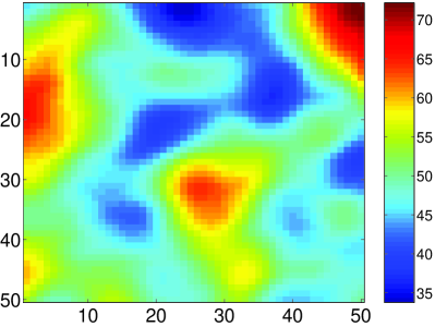
Figure 8: Synthetic random field with a Gaussian distribution $Z\sim N(m=50,\sigma=10)$ and Whittle-Matérn type correlations ($\nu=2.5$ and $\kappa=0.2$).

The correlation function is $c(r)=\sigma^{2}\,\frac{{2}^{1-\nu}}{\Gamma(\nu)}(\kappa r)^{\nu}K_{\nu}(\kappa r),$ where $\nu=2.5$ is the smoothness parameter, $\kappa=0.2$ is the inverse correlation length, and $K_{\nu}$ is the modified Bessel function of order $\nu$. The biggest difference in classification accuracy between the two models is obtained for $N_{c}=16$ and $p=0.33$: $F^{*}_{\rm{P-NN-MLC}}=35.1\%$, while $F^{*}_{\rm{I-NN-MLC}}=21.2\%$. We believe that the superior performance of the I-NN-MLC model results from the sequential strategy, in which points classified as $-1$ at lower levels are included in the sampling set at higher levels. Provided that the classification at lower levels is accurate, which is more likely for rather smooth and noise-free data (like the synthetic ones shown above), the included estimates can significantly improve the model’s performance. The sequential algorithm also reduces potential state degeneracy (i.e., spin configurations with the same energy). This feature is likely to occur in the spin models and it increases ambiguity in the identification of a particular spin configuration from the correlation energy. At the same time, the propagation of classification results from lower to higher levels can also be a weakness of the sequential algorithm, since low level classification errors influence the higher levels.

6 Conclusions and future research

We presented non-parametric approaches for spatial classification, inspired from the Ising and the Potts spin models, with a sequential and simultaneous classification strategy, respectively. The concept is based on the idea of matching the normalized correlation energies calculated from discretized data over the sampling grid and the entire area of interest. The matching is performed using Monte Carlo simulations, conditional on the sample values. The main advantage of the models is that they do not have any hypeparameters that need tuning; hence the classification is automatic, objective, competitive (in accuracy) and computationally efficient. The proposed methods are applicable to non-Gaussian distributions. In addition, they can incorporate non-stationary data, because even with a constant coupling strength the spin interactions imply a local impact of the sample values.

The future research includes the extension to scattered sampling patterns. One possible way is to define the interaction constant $J_{ij}$ in the Hamiltonians (3.1-3.2) through a kernel function (such as the radial basis function), and the interaction neighborhood (nearest neighbors), for example, as pairs of points whose Voronoi cells have a common boundary. Another way is to first use a simple interpolation method to place the irregularly spaced points on a regular grid with a specified resolution and then proceed as in the current study. The latter approach would allow vectorization and preserve the computational efficiency. Further possible extensions of the current models could also include further-neighbor or/and “higher-order” (e.g., three-point) correlation energy in the respective Hamiltonians. We could expect some elimination of the degeneracy, witnessed in the present models, and more faithful characterization of the nature of the spatial dependance. Both effects should contribute to the improvement of the classification performance. It would also be interesting to consider data sets with different patterns of missing data and investigate the effect of various gap patterns. Finally, it remains to be seen if the proposed methods can be used in the case of data sets containing a small number of extreme values, for example, two or three unusually elevated values detected by a monitoring network in the case of a radioactivity release.

References

References

- [1] P. M. Atkinson and N. J. Tate, (Eds.), Advances in Remote Sensing and GIS Analysis (John Wiley & Sons, 1999).
- [2] H. Wackernagel, Multivariate Geostatistics (Springer, 2003).
- [3] K. A. Hawick, Proc. of High Performance Computing and Networks Europe. LNCS 1401 (Springer, 1998).
- [4] P. J. Diggle and P. J. Ribeiro, Model-based Geostatistics. Series: Springer Series in Statistics (Springer, 2007).
- [5] D. T. Hristopulos, SIAM Journal in Scientific Computation 24, 2125 (2003).
- [6] R. N. Mantegna and H. E. Stanley, An Introduction to Econophysics: Correlations and Complexity in Finance (Cambridge University Press, Cambridge, 1999).
- [7] J. P. Bouchaud and M. Potters, Theory of Financial Risk (Cambridge University Press, Cambridge, 2000).
- [8] J. P. Bouchaud, P. Alstrom, and K. B. Lauritsen, (Eds.), Application of Physics in Financial Analysis, Int. J. Theor. Appl. Finance (special issue) 3 (2000).
- [9] M. Kardar, A. L. Stella, G. Sartoni, and B. Derrida, Phys. Rev. E 52, R1269 (1995).
- [10] M. Wouts, Stochastic Process. Appl., Online, arXiv:0705.1630v2, (2007).
- [11] Y. G. Zhenga, C. Lub, Y. W. Maib, H. W. Zhanga, and Z. Chenc, Science and Technology of Advanced Materials 7, 812 (2006).
- [12] F. Graner and J. A. Glazier, Physical Review Letters 69, 2013 (1992).
- [13] J. Besag, Journal of the Royal Statistical Society, Series B 48 259 (1986).
- [14] G. Gimel’farb, Pattern Recognition Letters 20 1123 (1999).
- [15] Z. Kato and Ting-Chuen Pong, Image and Vision Computing 24 1103 (2006).
- [16] J. Zhao and X. Wang, Third International Conference on Natural Computation, (ICNC 2007).
- [17] K. Tanaka and T. Morita, Physics Letters A 203, 122 (1995).
- [18] M. Blatt, S. Wiseman, and E. Domany, Physical Review Letters 76, 3251 (1996).
- [19] B. V. Dasarathy,(Ed.), Nearest Neighbor (NN) Norms NN Pattern Classification Techniques, (IEEE Computer Society Press, Los Alamitos, CA, 1991).
- [20] V. S. Cherkassky and D. Gehring, IEEE Trans. on Neural Networks 7, 969 (1996).
- [21] C. L. Y. Yeong and S. Torquato, Physical Review E 57, 495 (1998).
- [22] C. L. Y. Yeong and S. Torquato, Physical Review E 58, 224 (1998).
- [23] B. M. McCoy, T. T. Wu, The Two-Dimensional Ising Model (Harvard University Press, Cambridge Massachusetts, 1973).
- [24] F. Y. Wu, Reviews of Modern Physics, 54, 235 (1982).
- [25] C. H. Papadimitriou and K. Steiglitz Combinatorial Optimization (Prentice Hall, 1982).
- [26] Isaak E. and Srivastava R., An Introduction to Applied Geostatistics, Oxford University Press, New York, 1989.
- [27] P. Whittle, Biometrika, 41, 434 (1954).