Application of the Lifshitz theory to poor conductors

Abstract

The Lifshitz formula for the dispersive forces is generalized to the materials, which cannot be described with the local dielectric response. Principal nonlocality of poor conductors is related with the finite screening length of the penetrating field and the collisional relaxation; at low temperatures the role of collisions plays the Landau damping. The spatial dispersion makes the theory self consistent. Our predictions are compared with the recent experiment. It is demonstrated that at low temperatures the Casimir-Lifshitz entropy disappears as $T$ in the case of degenerate plasma and as $T^{2}$ for the nondegenerate one.

The Casimir-Lifshitz force is a dispersion interaction of electromagnetic origin acting between neutral bodies without permanent polarizations. The original Casimir formula Cas48 for the force between ideal metals was extended to real materials by Lifshitz and coworkers Lif55 ; DLP ; LP9 . Recently there was considerable progress in the experimental verification of the theory (see review Cap07 and references therein) and various applications to nanosciences were discussed Cap07 . The Lifshitz theory is extensively accepted as a common tool to deal with dispersive forces in physics, biology, chemistry, and technology.

The zero temperature contribution to the force originating from quantum fluctuations of the electromagnetic field is well understood. On the contrary, the classical or high temperature part of the thermal contribution (no dependence on $\hbar$) is the source of constant controversies. There is no continuous transition for the forces between ideal metals and real metals Bos00 . It is related with the transparency of real metals for s-polarized (transverse electric) low frequency field. It was found that for real metals there is a thermodynamic problem Bez02 : the Casimir-Lifshitz entropy is not going to zero at $T\rightarrow 0$. This problem is still in debate (for the latest publications see Nernst ) but a new controversy for poor conductors emerged Gey05 . In this case the reflection coefficient for p-polarization (transverse magnetic) is discontinuous in the transition from zero to arbitrarily small conductivity. This discontinuity again breaks the Nernst heat theorem. Obvious contradiction to the common sense shows that some important physics is missed.

In this paper we demonstrate that account for the spatial dispersion of the materials resolves the problems and make the theory self consistent. We formulate the condition at which the Lifshitz formula can be extended to the description of the forces between nonlocal materials. Special attention is paid to the case of poor conductors because the nonlocal effects are more important for them than for dielectrics or good metals.

For dielectrics the nonlocality can be neglected due to the absence of free charges except maybe the range near polariton resonances. For metals the local approximation is good because of the very short Thomas-Fermi screening length. Spatial dispersion for metals is important at low temperatures when the mean free path for electrons becomes larger than the field penetration depth and the anomalous skin effect plays role Sve03 ; Ser05 ; Sve05 .

Recently it was demonstrated by Pitaevskii Pit08 that the classical part of the Casimir-Polder force between a bad conductor and an atom is essentially nonlocal due to the finite screening length of free charges (Debye length). In Ref. Pit08 the force was found in the large distance limit. The formula for the force interpolates between good metals and dielectrics. It depends on the density of free carriers via the Debye length $l_{D}$.

The most general theory allowing the spatial dispersion was developed by Barash and Ginzburg Bar75 . The force was found to have an additional term in comparison with the Lifshitz formula related with the nonlocal material response. On this bases it was concluded in Ref. Kli07 that the Lifshitz formula cannot be used in the nonlocal case. However, this conclusion does not follow from Bar75 . The Lifshitz formula can be applied at least for plasma-like media. It was demonstrated Bar75 that if the long range interaction is taken into account in the plasma dielectric functions to the first order in the coupling constant $e^{2}$, then the Lifshitz formula holds true.

Below it is shown that the dielectric functions of the plasmas in metals and semiconductors calculated in the random phase approximation (RPA) can be used with the Lifshitz formula and give sufficient description of these materials for evaluation of the Casimir-Lifshitz force.

To account for the nonlocal response of metals it is possible Esq04 ; Ser05 to use the RPA (electrons are independent but respond not to the external field but to the screened one Ash76 ). This simple choice is good in the weak-coupling regime (rarefied plasma), but the plasmas in real metals are actually strongly coupled. However, significant deviations from RPA appear at large wavenumbers $k\sim k_{F}$ Gor80 , where $k_{F}$ is the Fermi wavenumber. For the bodies separated by the distance $a$ the important wavenumbers are $k\sim 1/a\ll k_{F}$. For this reason the use of the RPA dielectric functions is justified.

We can use the same approach to construct the nonlocal response of nondegenerate semiconductors. The difference with metals is that now electrons (holes) have to be considered as nondegenerate plasma and instead of the Fermi-Dirac distribution the Boltzmann distribution can be used. Technically the problem is equivalent to the weak-coupled nondegenerate plasma, for which one can use the textbook result LP10 .

Generalizing the situation we can consider two classes of plasmas: degenerate and nondegenerate. The first class (I) describes materials for which density of free charged particles stays finite at $T=0$. Metals, semimetals, degenerate semiconductors etc. belong to this class. Materials with the energy gap, for which density of free charges disappears with $T$ belong to the second class (II). Representatives of this class are nondegenerate semiconductors, ionic conductors, many disordered materials etc.

In the nonlocal case the dielectric function becomes a tensor, which has two independent components: transversal $\varepsilon_{t}$ and longitudinal $\varepsilon_{l}$ with respect to the wave vector ${\bf k}$. For very small relaxation frequency $\gamma\rightarrow 0$ (collisionless plasma) in RPA these components are

$$\varepsilon_{t,l}(\omega,k)=\varepsilon_{0}(\omega)-\frac{\omega_{p}^{2}}{\omega(\omega+i\gamma)}f_{t,l}(x).$$ (1)

Here the first term $\varepsilon_{0}(\omega)$ is introduced to account for the interband transitions since these processes are beyond the (quasi)free electron model. The variable $x$ is

$$x=\frac{\omega+i\gamma}{vk},\ \ \ v=\left\{\begin{array}[]{c}v_{F},\ {\rm for}\ I,\\ \sqrt{\frac{2T}{m^{*}}},\ {\rm for}\ II,\end{array}\right.$$ (2)

where $m^{*}$ is the effective mass of the charge carrier (electron or hole) and $v_{F}$ is the Fermi velocity. The plasma frequency $\omega_{p}$ in (1) and the Debye wavenumber $k_{D}$ (see below) are defined as

$$\omega_{p}=\sqrt{\frac{4\pi e^{2}N}{m^{*}}},\ \ \ k_{D}=\left\{\begin{array}[]{c}\sqrt{\frac{12\pi e^{2}N}{m^{*}v_{F}^{2}}}\ {\rm for}\ I,\\ \sqrt{\frac{4\pi e^{2}N}{T}}\ {\rm for}\ II,\end{array}\right.$$ (3)

where $N$ is the density of carriers. Note that $\varepsilon_{t}$ and $\varepsilon_{l}$ are of the first order in $e^{2}$ and can be used with the Lifshitz formula. The functions $f_{t,l}(x)$ are different for each class and can be found in the textbooks (see, for example, LP10 ). For the class I they are

$$f_{t}(x) = \frac{3x}{2}\left[x-\frac{1}{2}(x^{2}-1)\ln\frac{x+1}{x-1}\right],$$

$$f_{l}(x) = 3x^{2}\left[-1+\frac{x}{2}\ln\frac{x+1}{x-1}\right].$$ (4)

For the class II these functions are

$$f_{t}(x)=-F(x),\ \ \ f_{l}(x)=-2x^{2}\left(1+F(x)\right),$$ (5)

where $F(x)$ is defined as

$$F(x)=\frac{x}{\sqrt{\pi}}\int\limits_{-\infty}^{\infty}dz\frac{e^{-z^{2}}}{z-x}.$$ (6)

The dielectric functions (1) can be generalized to the case of finite relaxation frequency $\gamma$. For the transverse component $\varepsilon_{t}(\omega,k)$ this is an easy task since the collision integral in the relaxation time approximation gives the same result as (1) but with the finite value of the relaxation frequency $\gamma$.

Different procedure has to be used to account for the finite relaxation time in $\varepsilon_{l}(\omega,k)$. The longitudinal field influences the charge distribution. In this case the relaxation of the perturbed distribution toward ”equilibrium” will be to the local state of charge imbalance and not to the uniform distribution War60 . Mermin Mer70 used this idea to generalize $\varepsilon_{l}(k,\omega)$ calculated in RPA to the finite relaxation time:

$$\tilde{\varepsilon}_{l}(\omega,k)=\varepsilon_{0}(\omega)+\frac{(1+i\frac{\gamma}{\omega})\left[\varepsilon_{l}(\omega+i\gamma,k)-\varepsilon_{0}(\omega)\right]}{1+i\frac{\gamma}{\omega}\frac{\varepsilon_{l}(\omega+i\gamma,k)-\varepsilon_{0}(\omega)}{\varepsilon_{l}(0,k)-\varepsilon_{0}(0)}},$$ (7)

where we denote the dielectric functions with the finite relaxation frequency as $\tilde{\varepsilon}_{t,l}$.

The dielectric functions $\tilde{\varepsilon}_{l,t}(k,\omega)$ are defined for an infinite medium. The spatial dispersion close to the body surface needs special attention. Strictly speaking one can define the nonlocal dielectric function only for infinite body, but in special cases of specular and diffuse reflection of electrons on the surface of the body it is also possible to do. We will consider here the case of specular reflection. An electron reflected from the interface with vacuum cannot be distinguished from that coming from a fictitious medium on the vacuum side. In this way the specular condition continues the medium with the interface to the infinite medium.

For actual evaluation of the force in the case of materials with the spatial dispersion it is more convenient to use the surface impedances instead of the dielectric functions Esq04 . These impedances are connected with the dielectric functions by the relations

$$Z_{s}(q,\omega) = \frac{i\omega}{\pi c}\int\limits_{-\infty}^{\infty}\frac{dk_{z}}{\frac{\omega^{2}}{c^{2}}\tilde{\varepsilon}_{t}-k^{2}},$$ (8)

$$Z_{p}(q,\omega) = \frac{i\omega}{\pi c}\int\limits_{-\infty}^{\infty}\frac{dk_{z}}{k^{2}}\left[\frac{q^{2}}{\frac{\omega^{2}}{c^{2}}\tilde{\varepsilon}_{l}}+\frac{k_{z}^{2}}{\frac{\omega^{2}}{c^{2}}\tilde{\varepsilon}_{t}-k^{2}}\right],$$ (9)

where the wave vector is ${\bf k}=(q_{x},q_{y},k_{z})$ and the $z$-axis is perpendicular to the body surface.

The reflection coefficients are expressed via the impedances as

$$r_{s}(q,\omega)=-\frac{\omega/ck_{0}-Z_{s}}{\omega/ck_{0}+Z_{s}},\ \ \ r_{p}(q,\omega)=\frac{ck_{0}/\omega-Z_{p}}{ck_{0}/\omega+Z_{p}},$$ (10)

where $k_{0}=\sqrt{\omega^{2}/c^{2}-q^{2}}$. Now we can use the reflection coefficients (10) in the Lifshitz formula. This formula is usually presented via the imaginary Matsubara frequencies $\omega\rightarrow i\zeta_{n}=i2\pi Tn/\hbar$:

$$F(a,T)=\frac{T}{\pi}\sum\limits_{\mu=s,p}\sum\limits_{n=0}^{\infty}{}^{\prime}\int\limits_{0}^{\infty}dqq|k_{0}|\frac{r_{\mu 1}r_{\mu 2}e^{-2|k_{0}|a}}{1-r_{\mu 1}r_{\mu 2}e^{-2|k_{0}|a}},$$ (11)

where $r_{\mu i}=r_{\mu i}(q,\zeta_{n})$ is the reflection coefficient of the body $i$ ($i=1,2$) for the polarization $\mu$ ($\mu=s,p$).

Let us consider the influence of the spatial dispersion on the force. When $T$ is around room temperature typical values of the parameters are $\gamma\sim 10^{13}-10^{14}\;rad/s$, $k\sim 1/a$, and $v\lesssim 10^{6}\;m/s$. Then the natural value of $x$ in (2) is large, $|x|\gg 1$, for most of the materials in the interesting distance range 10-1000 nm. In this limit both dielectric functions become local:

$$\tilde{\varepsilon}_{t}=\tilde{\varepsilon}_{l}(k,i\zeta_{n})=\varepsilon_{0}(i\zeta_{n})+\frac{\omega_{p}^{2}}{\zeta_{n}\left(\zeta_{n}+\gamma\right)},\ \ \ n>0$$ (12)

This is true, however, for $n>0$. In the case $n=0$ or $\zeta\rightarrow 0$ the result is different:

$$\tilde{\varepsilon}_{t}(k,i\zeta)=\varepsilon_{0}+\frac{\omega_{p}^{2}}{\zeta\gamma},\ \ \ \tilde{\varepsilon}_{l}(k,i\zeta)=\varepsilon_{0}+\frac{k_{D}^{2}}{k^{2}},$$ (13)

where $\varepsilon_{0}=\varepsilon_{0}(0)$. In the real frequency domain this limit is realized for $\omega\ll\gamma$. As one can see $\tilde{\varepsilon}_{l}$ demonstrates the nonlocal character.

We can conclude that at room temperature all the $n>0$ terms in (11) can be calculated with the local dielectric functions. The $n=0$ term has to be corrected to take into account the nonlocality. Calculating the impedances (8) and (9) with the functions (13) and substituting them into the reflection coefficients (10) one finds

$$r_{s}\rightarrow 0,\ \ \ r_{p}=\frac{\varepsilon_{0}\sqrt{q^{2}+k_{D}^{2}/\varepsilon_{0}}-q}{\varepsilon_{0}\sqrt{q^{2}+k_{D}^{2}/\varepsilon_{0}}+q}.$$ (14)

Here $r_{s}$ is zero because in the static limit $s$-polarized field is reduced to pure magnetic field, which penetrates the nonmagnetic material. One can see that $r_{p}$ interpolates between a good metal and a pure dielectric. Really, important values of $q$ are $q\sim 1/a$, then for $a\ll l_{D}=\sqrt{\varepsilon_{0}}/k_{D}$ the reflection coefficient $r_{p}=(\varepsilon_{0}-1)/(\varepsilon_{0}+1)$ is as for a dielectric with the permittivity $\varepsilon_{0}$. In the opposite limit $r_{p}=1$ corresponds to good metals.

In the local theory the $n=0$ term in the Lifshitz formula (11) can be presented in the Lifshitz form DLP

$$F_{0}(a,T)=\frac{T}{16\pi a^{3}}\int\limits_{0}^{\infty}dx\frac{x^{2}Re^{-x}}{1-Re^{-x}},$$ (15)

where $R=r_{p1}r_{p2}$ is just a constant. For example, for two dielectrics with permittivities $\varepsilon_{1}$ and $\varepsilon_{2}$ it is

$$R=\frac{(\varepsilon_{1}-1)(\varepsilon_{2}-1)}{(\varepsilon_{1}+1)(\varepsilon_{2}+1)}.$$ (16)

In the more general theory, which takes into account the spatial dispersion of the materials, the $n=0$ term can be presented in the same form (15) but now $R$ is not a constant but a function of $q$ as follows from (14). Introducing for each material the parameter $\xi_{i}=2a/l_{iD}$ ($i=1,2$) we can present $R=r_{p1}r_{p2}$ as

$$R(x)=\frac{\varepsilon_{1}\sqrt{x^{2}+\xi^{2}_{1}}-x}{\varepsilon_{1}\sqrt{x^{2}+\xi^{2}_{1}}+x}\cdot\frac{\varepsilon_{2}\sqrt{x^{2}+\xi^{2}_{2}}-x}{\varepsilon_{2}\sqrt{x^{2}+\xi^{2}_{2}}+x}.$$ (17)

From (15) and (17) we can reproduce the main formula (34) in Pit08 . For that in the large distance limit we can consider the second body as rarefied $\varepsilon_{2}-1\ll 1$, $\xi_{2}\rightarrow 0$ and calculate the atom-body potential as $V=-F_{0}(a,T)$.

Our analysis of the Casimir-Lifshitz force for poor conductors at room temperature can be applied for the description of a recent experiment Che07a ; Che07b , the result of which did not found a reasonable explanation yet. In this experiment a p-type silicon membrane with the carrier density $N\approx 5\cdot 10^{14}\ cm^{-3}$ was excited by the laser light. The density of photogenerated carriers was varied in the range $N_{ph}=(1.4-2.1)\cdot 10^{19}\ cm^{-3}$. The force difference in the presence and in the absence of laser light was measured with an atomic force microscope (AFM) as a function of the distance between the membrane and the sphere at the end of the cantilever. It was found that the experimental results agree well with the dielectric membrane rather than with the semiconducting one. On this basis a controversial conclusion was made that one has to disregard the finite conductivity of silicon when the Casimir-Lifshitz force is evaluated.

The controversy manifests itself in the local variant of the theory as discontinuity of the $n=0$ term in the Lifshitz formula. For a dielectric (body 1) and metal (body 2) this term is given by (15) with $R=(\varepsilon_{1}-1)/(\varepsilon_{1}+1)$. Even for infinitely small conductivity of the dielectric this term has to be calculated with $R=1$ and the result will coincide with the $n=0$ term for two metals. The nonlocality smooth out this discontinuity allowing continuous transition from dielectric to metal in accordance with the common sense.

Figure 1 shows the experimental data for two densities of the photogenerated carriers Note that $N_{ph}$ in both cases are the same within the errors. Comparing figures 1(a) and 1(b) one can see that the experiment can hardly distinct between the nonlocal theory and the local theory with zero conductivity of Si.

The controversies of the local theory are closely related with the behavior of the entropy at $T\rightarrow 0$. Let us check the Nernst heat theorem in the nonlocal case. At low temperatures we cannot use the dielectric functions (12) and (13) since the variable $|x|$ now is not large. Actually, when $T$ is sufficiently small, the opposite limit is realized $|x|\ll 1$, for which the nonlocal effects are strong. This is because $\gamma(T)$ decreases with $T$ faster than linearly. Important imaginary frequencies contributing to the temperature dependent part of the free energy are $\zeta\sim 2\pi T/\hbar$. Now the nonlocality is important for many terms in the sum (11). In this limit the dielectric functions are

$$\tilde{\varepsilon}_{t}(i\zeta,k)=\varepsilon_{0}(i\zeta)+\frac{\alpha\omega_{p}^{2}}{\zeta vk},\ \ \ \tilde{\varepsilon}_{l}(i\zeta,k)=\varepsilon_{0}(i\zeta)+\frac{k_{D}^{2}}{k^{2}}.$$ (18)

Here we suppressed the index $n$ and $\alpha$ is $3\pi/4$ for the class I and $\sqrt{\pi}$ for II. Note that $\gamma$ falls out from the result; its role plays the Landau damping frequency $vk$.

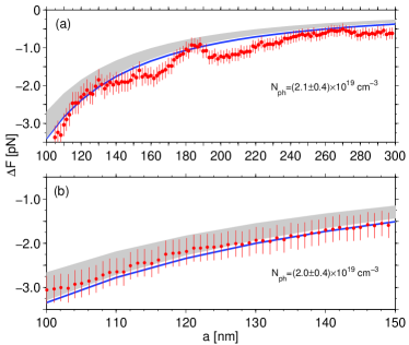
Figure 1: (Color online) Difference of the forces on the low-doped Si membrane in the presence and in the absence of photogenerated carriers (dots with bars). The gray stripes are predictions of this work accounted for errors in $N_{ph}$. The blue curves are predictions based on pure dielectric Si for the central values of $N_{ph}$. (a) and (b) correspond to different laser powers exciting the carriers (see Che07b ).

Luckily there is no need to calculate the free energy with (18); all the work was done before. For the class I materials the calculations were performed in Sve05 but the distance dependent leading term was presented in Sve06 :

$${\cal F}\approx-0.0193\;T^{2}\frac{a\omega_{p}^{2}}{\hbar v_{F}c^{2}},\ \ \ T\ll\frac{\hbar v_{F}c^{2}}{12\pi^{2}\omega_{p}^{2}a^{3}}.$$ (19)

The spatial dispersion changes the behavior of the free energy with $T$: instead of linear as in the local theory Bez02 it becomes quadratic. It ensures the right behavior of the entropy $S\sim+T$.

Different situation is realized for the class II materials. In this case the density of carriers $N(T)$ is a function of temperature. Due to presence of the energy gap for these materials at $T\rightarrow 0$ the dependence is exponential $N(T)\sim e^{-\Delta/T}$, where $\Delta$ is the gap. Because both parameters $\omega_{p}^{2}$ and $k_{D}^{2}$ are proportional to $N(T)$ their effect in the dielectric functions (18) is exponentially small. This conclusion is also true for the hopping mechanism of conductivity. In this case the effective density of charges, which are able to move, is $\sim e^{-\Delta/T}$ Lin79 . In the limit $T\rightarrow 0$ the class II materials become pure dielectric. For dielectrics the entropy disappears with $T$ as $S\sim T^{2}$ Gey05 .

In conclusion, the Lifshitz formula was generalized to materials, which cannot be described as local media. The spatial dispersion naturally resolves paradoxes appearing in the theory for local materials with finite conductivity.

When this work was finished a preprint Dal08 appeared where the Lifshitz theory was generalized to semiconductors. Ideologically the approach is similar to ours but less general and technically different.

Fruitful discussion with L. P. Pitaevskii is appreciated.

References

- (1) H.B.G. Casimir, Proc. K. Ned. Akad. Wet. 51, 793 (1948).
- (2) E.M. Lifshitz, Dokl. Akad. Nauk SSSR 100, 879 (1955).
- (3) I.E. Dzyaloshinskii, E.M. Lifshitz and L.P. Pitaevskii, Advances in Physics 38, 165 (1961).
- (4) E. M. Lifshitz and L. P. Pitaevskii, Statistical Physics (Pergamon Press, Oxford, 1980) Pt. 2.
- (5) F. Capasso, J. N. Munday, D. Iannuzzi, and H. B. Chan, IEEE J. Sel. Top. Quantum Electron. 13, 400 (2007).
- (6) M. Boström and B.E. Sernelius, Phys. Rev. Lett. 84, 4757 (2000).
- (7) V. B. Bezerra, G. L. Klimchitskaya, and V. M. Mostepanenko, Phys. Rev. A 65 , 052113 (2002).
- (8) G. L. Klimchitskaya and V. M. Mostepanenko, Phys. Rev. E 77, 023101 (2008); J. S. Høye, I. Brevik, S. A. Ellingsen, and J. B. Aarseth, Phys. Rev. E 77, 023102 (2008).
- (9) B. Geyer, G. L. Klimchitskaya, and V. M. Mostepanenko, Phys. Rev. D 72, 085009 (2005).
- (10) V. B. Svetovoy and M. V. Lokhanin, Phis. Rev. A 67, 022113 (2003).
- (11) Bo E. Sernelius, Phys. Rev. B 71, 235114 (2005); Phys. Rev. B 75, 036102 (2007).
- (12) V.B. Svetovoy and R. Esquivel, Phys. Rev. E 72, 036113 (2005).
- (13) L. P. Pitaevskii, arXiv: 0801.0656.
- (14) Y. S. Barash and V. L. Ginzburg, Usp. Fiz. Nauk 116, 5 (1975) [Sov. Phys. Uspekhi 18, 305 (1975)].
- (15) G. L. Klimchitskaya and V. M. Mostepanenko, Phys. Rev. B 75, 036101 (2007).
- (16) R. Esquivel and V. B. Svetovoy, Phys. Rev. A 69, 062102 (2004).
- (17) N. W. Ashcroft and N. D. Mermin, Solid State Physics (Thomson Learning, Toronto, 1976).
- (18) V. D. Gorobchenko and E. G. Maksimov, Usp. Fiz. Nauk 130, 65 (1980) [Sov. Phys. Usp. 23, 35 (1980)].
- (19) E. M. Lifshitz and L. P. Pitaevskii, Physical Kinetics (Pergamon Press, Oxford, 1981).
- (20) V.B. Svetovoy and R. Esquivel, J. Phys. A: Math. Gen. 39, 6777 (2006).
- (21) J. L. Warren and R. A. Ferrell, Phys. Rev. 117, 1252 (1960).
- (22) N. D. Mermin, Phys. Rev. B 1, 2362 (1970).
- (23) F. Chen, G. L. Klimchitskaya, V. M. Mostepanenko, and U. Mohideen, Opt. Express 15, 4823 (2007).
- (24) F. Chen, G. L. Klimchitskaya, V. M. Mostepanenko, and U. Mohideen, Phys. Rev. B 76, 035338 (2007).
- (25) M. E. Lines, Phys. Rev. B 19, 1183 (1979).
- (26) D. A. R. Dalvit and S. Lamoreaux, arXiv: 0805.1676.