Radio Bursts Associated with Flare and Ejecta in the 13 July 2004 Event

Abstract

We investigate coronal transients associated with a GOES M6.7 class flare and a coronal mass ejection (CME) on 13 July 2004. During the rising phase of the flare, a filament eruption, loop expansion, a Moreton wave, and an ejecta were observed. An EIT wave was detected later on. The main features in the radio dynamic spectrum were a frequency-drifting continuum and two type II bursts. Our analysis shows that if the first type II burst was formed in the low corona, the burst heights and speed are close to the projected distances and speed of the Moreton wave (a chromospheric shock wave signature). The frequency-drifting radio continuum, starting above 1 GHz, was formed almost two minutes prior to any shock features becoming visible, and a fast-expanding piston (visible as the continuum) could have launched another shock wave. A possible scenario is that a flare blast overtook the earlier transient, and ignited the first type II burst. The second type II burst may have been formed by the same shock, but only if the shock was propagating at a constant speed. This interpretation also requires that the shock-producing regions were located at different parts of the propagating structure, or that the shock was passing through regions with highly different atmospheric densities. This complex event, with a multitude of radio features and transients at other wavelengths, presents evidence for both blast-wave-related and CME-related radio emissions.

1 Introduction

Decimetric–metric radio emission is usually associated with plasma waves excited by accelerated electrons, where the observed emission frequency is directly related to the plasma density in the affected region [Melrose (1980)]. Fast-drifting structures in radio dynamic spectra, such as type III bursts, are normally attributed to electron beams propagating outward in the solar atmosphere. The type III burst-associated acceleration usually happens in connection with flaring processes, by for example, reconnecting field lines. A slower drift and a broader instantaneous emission band in a radio burst can indicate a moving shock front that accelerates electrons. Some of these bursts can be classified as type II bursts, in particular when both fundamental and second harmonic emission bands are visible (e.g., Nelson and Melrose, 1985; Mann, Classen, and Aurass, 1995; Cairns et al., 2003). Although type II bursts indicate the existence of shock waves, their origin is not always so clear. Shocks can basically be flare related or coronal mass ejection (CME) related, but coronal (metric) type II bursts do not necessarily have the same origin as the longer wavelength (interplanetary) type II bursts (Mancuso and Raymond, 2004; Cane and Erickson, 2005; Lin, Mancuso, and Vourlidas, 2006, and references therein).

Theoretically, shocks can be freely propagating (blast) waves, piston-driven shocks formed either at the nose or the flanks of an expanding body, or bow shocks ahead of a projectile Warmuth (2007). A freely propagating shock can also develop if a piston stops or slows down considerably. One characteristic of piston-driven shocks is that the speed of the propagating shock is different from the speed of the driver, and the shock speed should be higher. For bow shocks ahead of a projectile, the speeds should be roughly the same, see, for example, vrsnak05.

Frequency-drifting continuum emissions at centimeter to meter wavelengths, also known as type IV bursts, have been associated with outward moving plasmoids, see review on solar radio emission in, for example, dulk85. At decimetric wavelengths, the usually smooth type IV continuum may include pulsating structures Kundu (1965). In some cases decimetric pulsating structures can be taken as precursors to type II bursts Klassen et al. (1999), and identified as a signature of reconnection processes above expanding soft X-ray loops Klassen, Pohjolainen, and Klein (2003).

This study presents a flare–CME event on 13 July 2004, during which a rich variety of radio bursts were observed from centimeter to meter wavelengths. In this paper, we concentrate on the type II and type IV bursts observed at decimeter–meter wavelengths. During this event, quasi-periodic pulsations were observed in microwaves and decimeter waves, but they will be discussed in another paper. We compare the timing, heights, and structural evolution of the observed features and discuss conditions that are needed for the radio emissions to appear.

2 Observations

Full-disk EUV images at 195 Å  during the 13 July 2004 event were provided by the SOHO EUV Imaging Telescope (EIT) instrument Delaboudinière et al. (1995), and high resolution, limited field of view images at 171 Å by the Transition Region and Coronal Explorer (TRACE) satellite Handy et al. (1999). Big Bear Solar Observatory (BBSO; part of the global high-resolution H$\alpha$ network at 656.3 nm wavelength) observed the event in H$\alpha$ with a cadence of 1 – 3 images per minute. White-light coronagraph images were obtained from the SOHO Large Angle Spectrometric Coronagraph (LASCO) instrument Brueckner et al. (1995), and the Reuven Ramaty High Energy Solar Spectroscopic Imager (RHESSI) provided hard X-ray data Lin et al. (2002). Coronal mass ejections are listed in the LASCO CME Catalog at http://cdaw.gsfc.nasa.gov/CME_list/.

Nobeyama radio polarimeters (NoRP) observed radio flux densities at seven single frequencies between 1 and 80 GHz Nakajima et al. (1985). Simultaneous radio imaging was obtained at 17 and 34 GHz with the Nobeyama Radioheliograph, NoRH Nakajima et al. (1994). At decimetric-metric wavelengths dynamic spectra were recorded by the HiRAS radiospectrograph, which covers a frequency range from 25 MHz to 2.5 GHz, and with the Radio Solar Telescope Network (RSTN) instruments operated by the U.S. Air Force at four different sites, observing at 25–180 MHz. For comparison, NoRP and HiRAS have two overlapping frequencies, at 1 and 2 GHz.

2.1 Flare, Ejecta and EIT Wave

On 13 July 2004 a GOES M6.7 class flare was observed in the NOAA active region 10646, located at N14 W45. The GOES soft X-ray flux started to rise at 00:08 UT, and there were two impulsive rises after that, at 00:11:40 and 00:13:05 UT. Flux peak was recorded at 00:17 UT.

The first signs of a filament eruption were visible in the TRACE EUV image at 00:12:45 UT. At about the same time, quasi-periodic pulsations in hard X-rays and microwaves started. H$\alpha$ flare ribbons appeared in the images at 00:14:25 UT.

A large EUV loop structure was observed over the active region before the flare started, and this structure began to rise at about 00:14 UT. The arc-shaped front is indicated with white arrows in the TRACE difference images in Figure 1 (top row). The structure moved outside the TRACE field of view at about 00:18 UT. The projected plane-of-the-sky rise velocity of the front is estimated to be between 235 and 330 km s^-1. Some caution is needed when interpreting propagating loop-like features, as some of them can be shock waves driven by erupting filaments Pomoell, Vainio, and Kissmann (2008), but in this case the pre-event EUV loop and the slow rise velocity suggest that it was a rising loop.

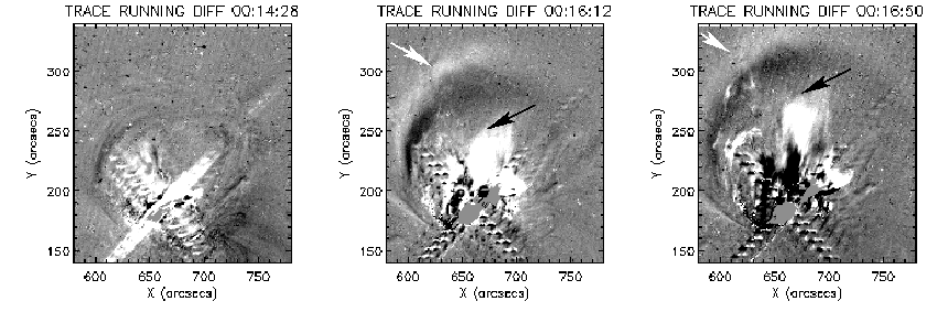
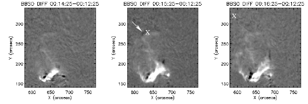
Figure 1.: Top: TRACE difference images showing a rising loop-like structure (white arrows; projected speed 235 – 330 km s^-1) above the active region at N14W45, and a following ejecta (black arrows; projected speed of 660 km s^-1). Bottom: BBSO H$\alpha$ difference images of the same region. A chromospheric disturbance is observed near the location of the rising EUV loop-like structure (white arrow). Crosses mark the locations of the H$\alpha$ Moreton wave front (which are too faint to be observed in these images, see text for details).

At about 00:15 UT, below the rising loop-like structure, a bright EUV ejecta started to move upward. The ejecta front is indicated with black arrows in Figure 1 (top row). The projected rise speed is estimated to be about 660 km s^-1.

H$\alpha$ difference images show a disturbance at the chromospheric level at about 00:15 UT (at a location indicated with a white arrow in Figure 1, bottom row). This feature is very near the location of the EUV loop-like structure, and also near the front of a faint H$\alpha$ Moreton wave (Figure 1, with locations indicated with crosses); see details and a movie in grechnev08. The H$\alpha$ wave was propagating toward North–Northeast from the active region and the projected speed estimate is about 700 km s^-1. H$\alpha$ (Moreton) waves are generally thought to be direct signatures of propagating blast wave shocks in the chromosphere Uchida (1974).

Later on, the erupting H$\alpha$ filament was observed to move toward the Northwest. The filament trajectory, at three different times between 00:19 and 00:27 UT traced from the BBSO H$\alpha$ observations, is marked in Figure 2.

In the full-disk EUV images (SOHO EIT) brightenings and dimmed regions can be observed from 00:24 UT onward. The brightenings in the EIT difference images are the so-called EIT-waves Thompson et al. (1999), and we can estimate the wave front distances from the active region at two different times. The estimated (projected) speed of the front, measured from the running difference images at 00:24 and 00:36 UT, is approximately 300 km s^-1. Figure 2 shows the outlines of the farthermost fronts toward the Northeast at 00:24 and 00:36 UT, and also the backward-extrapolated front distance at 00:12 UT, if the wave speed had remained constant. However, in the EIT image at 00:12 UT no EIT wave can be detected. Either the EIT wave had formed some distance away from the active region or the wave had decelerated after formation. The rising EUV loop front locations at 00:14 and 00:17 UT, along with the erupting filament trajectory, are indicated in Figure 2 for comparison.

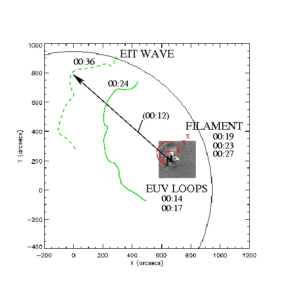
Figure 2.: EIT wave locations at 00:24 and 00:36 UT, with an estimate of the wave location at 00:12 UT if it had moved at a constant speed. Note that the EIT image at 00:12 UT does not show any signatures of an EIT wave. The expanding and rising loop-like structure observed by TRACE in EUV is shown in the insert image (outlined in black solid lines) and Xs mark the path of the erupting H$\alpha$ filament observed by BBSO.

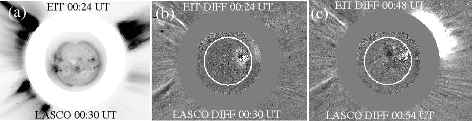
Figure 3.: LASCO C2 image at (a) 00:30 UT showing a strong streamer region in the Northwest direction. LASCO C2 running difference images at (b) 00:30 UT and (c) 00:54 UT, with the EIT difference images inside the occulted disk, showing the early evolution of the CME. (Images courtesy of the LASCO CME Catalog)

2.2 Coronal Mass Ejection

A CME was first detected in white-light in the LASCO C2 difference image at 00:54 UT, over the solar northwestern limb (Figure 3) at a heliocentric height of 3.07 $R_{\odot}$. In the previous LASCO image at 00:30 UT the CME front is not yet visible, but the SOHO EIT running difference image at 00:24 UT shows brightenings on the disk and above the limb in the same direction as the later-observed CME. In the pre-eruption images an intense streamer region is visible over the northwestern limb (Figure 3, left panel).

The projected plane-of-the-sky speed of the CME was approximately 450 km s^-1, measured from the LASCO images at 00:54 and 01:31 UT. Later on, the CME decelerated to a speed of about 400 km s^-1 (LASCO CME Catalog, linear fit to all later CME observations and second order fit to all data). The CME Catalog also lists another event during the same period, with a plane-of-the sky speed of 600 km s^-1, but from the LASCO images this leading edge is hard to identify.

2.3 Radio Emission

HiRAS radio dynamic spectrum shows that radio emission at decimetric–metric wavelengths consist of several emission features (Figure 4). First, it shows a faint, frequency-drifting continuum starting above 1 GHz. At 1 GHz, the continuum flux starts to rise at about 00:13:20 UT. Metric type III bursts that continue to decameter –hectometer wavelengths (Wind WAVES observations) are observed soon after the appearance of the drifting continuum. This indicates that at this early phase some field lines connected to the flaring region had opened, along which electrons could stream into the interplanetary space.

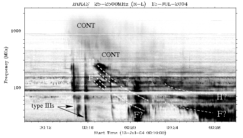
Figure 4.: HiRAS dynamic radio spectrum at 00:10 – 00:30 UT at 25 MHz – 2.5 GHz. At least two type II burst lanes, with emission at the fundamental (F) and second harmonic (H) frequencies, can be found in the spectrum. The emission lanes of the first type II burst are also band-split. Frequency-drifting continuum emission (labeled CONT) is visible below $\approx$ 2 GHz.

About three minutes after the start of continuum emission, a metric type II burst appears in the dynamic spectrum, at 00:16:40 UT. The burst shows emission both at the fundamental ($\approx$ 120 MHz) and second harmonic ($\approx$ 240 MHz) plasma frequencies. RSTN observations show that the emission lanes are band-split. Type II burst lanes are again observed at about 00:24 UT, now with emission at 50 MHz and just above 100 MHz. The emission bands of these bursts are outlined with dashed lines in Figure 4. In between these two burst lanes, we see a pair of bursts that look like disturbed type III emission. The lower emission patch is located around 40 MHz at 00:21 UT. There have been reports on disturbed type III burst lanes, possibly formed when outward-streaming electrons travel through a turbulent shock region Reiner et al. (2000); Lehtinen et al. (2008). So in our case the bursts probably trace the path of a propagating shock, when the shock no longer produces a continuous type II burst lane.

The frequency drift of the first visible type II burst is approximately 0.4 MHz s^-1. The drift rate of the second type II burst is about 0.1 MHz s^-1. Both values are within the usual 0.1 – 1.0 MHz s^-1 drift rate for typical type II bursts Nelson and Melrose (1985). No interplanetary type II bursts were observed associated with this event and no continuations of the metric type II bursts are visible in the dynamic spectra below 14 MHz (Wind WAVES observations).

3 Analysis of the Radio Emission

As plasma emission at the fundamental emission frequency $f_{p}$ is directly related to electron density $n_{e}$, we can use radio observations to estimate shock heights and speeds under the assumption of a coronal density model. One should be aware that height estimates depend strongly on the density models used. By calculating heights with more than one model and by taking into account the local coronal conditions, it is possible to give reliable height ranges for the emission sources. Different models and their characteristics are explained in detail in, for example, mann03, Appendix A of vrsnak04, and pohjolainen06. Direct observations of the densities of the pre-shocked coronal plasma are still rare, (e.g., Mancuso, 2007).

First, we calculate burst heights with three different atmospheric density models, which describe different types of atmospheres. The basic (1$\times$) Saito (1970) model is often used for equatorial regions in the corona, and also at large distances from the Sun, where active region densities no longer dominate. A two-times Newkirk (1961) density model is often used for densities in streamer regions and in active region solar corona. A ten-times Saito model can be used when a shock is propagating through high-density loops in the low corona. Since the LASCO images show a streamer region in the northwestern part of the Sun where the CME appears (Figure 3), high-density models should be more applicable. The estimated source heights at the start of the two bursts, and the derived velocities along the burst lanes, are given in Table 1.

Table 1.: Estimated heliocentric source heights and radio burst velocities

Time	$f_{p}$	$n_{e}$	Drift rate	$h$	$h$	$h$
UT	MHz	cm-3	MHz s-1	Saito	2$\times$Newkirk	10$\times$Saito
00:16:40	120	1.77$\times$108	0.4	1.09 $R_{\odot}$	1.30 $R_{\odot}$	1.46 $R_{\odot}$
Velocity				1100 km s-1	1700 km s-1	2300 km s-1
00:24:00	50	3.08$\times$107	0.1	1.34 $R_{\odot}$	1.68 $R_{\odot}$	2.0 $R_{\odot}$
Velocity				700 km s-1	1000 km s-1	1200 km s-1

We note that the radio source height given by the basic Saito model at 00:16:40 UT, is very near the projected EUV ejecta height at 00:16:50 UT (0.095 $R_{\odot}$ from the center of eruption). However, radio imaging observations at 164 MHz and frequencies above it usually show type II features near heights of 0.3 – 0.4 $R_{\odot}$ above the limb Klassen et al. (1999); Dauphin, Vilmer, and Krucker (2006). There are on-the-disk observations Klassen, Pohjolainen, and Klein (2003) of smaller projected distances from the flaring region, $\approx$ 0.2 $R_{\odot}$, but compared to these the height of $\approx$ 0.1 $R_{\odot}$ given by the basic Saito model for a source emitting at 120 MHz is uncommonly low. The heights given by the ten-times Saito model are also unrealistic at these frequencies, since the source heights are in conflict with the densities observed above active regions (see, e.g. Figure 2 in warmuth05).

The values in Table 1 suggest that the two type II bursts were propagating at different speeds. However, a change in the coronal conditions in between the bursts may change the speeds as well. For example, if the burst source first propagated in a low-density (Saito) atmosphere in the low corona and then entered a high-density streamer (2$\times$Newkirk) region, the shock speed would basically remain the same ($\approx$ 1 000 km s^-1), see the values in Table 1. Transitions between different regions are possible since the shock can be spatially large, but in this case a low-density (basic) Saito model atmosphere very low above the active region is not probable.

Type II burst velocities can also be estimated with the scale height method, see, e.g., demoulin00. Shock velocity $v$ can be calculated from the observed plasma frequency $f_{p}$ (MHz), the measured frequency drift $df/dt$ (MHz s^-1), and the scale height $H$ (km) as

$$v=2\frac{1}{f}\frac{df}{dt}H.$$ (1)

koutchmy94 discovered that the hydrostatic isothermal scale height in a 1.5 MK coronal temperature describes well the measured density profiles in the solar atmosphere, regardless of the base density. Since the source heights presented in Table 1 and the discussion on the values suggest that heights near 0.2 – 0.4 $R_{\odot}$ above the photosphere are possible for a radio source emitting at 120 MHz, we calculate the speeds using the scale height method. At a heliocentric height 1.2 $R_{\odot}$ the scale height is then 109 000 km. The emission frequency at the start of the first type II burst was 120 MHz and the observed frequency drift was 0.4 MHz s^-1, which gives a speed of 725 km s^-1. If we assume that the radio source was located higher, at 1.4 $R_{\odot}$, the scale height is 148 000 km and the corresponding speed is 985 km s^-1. If the shock propagated at 725 km s^-1 from a height 1.2 $R_{\odot}$, it would have reached the height of 1.66 $R_{\odot}$ at the time when the second type II burst started. But, the burst velocity calculated from the emission frequency of 50 MHz and the frequency drift of 0.1 MHz s^-1 at that height does not match with the first type II burst (being in fact higher). If, however, the second type II burst originated from a lower height, at 1.55 $R_{\odot}$, the calculated shock speeds for the first and second type II bursts would be the same. This implies that a deceleration of the shock would not be able to produce the observed frequency drift of the second type II burst, but a driver propagating at a constant speed and producing shocks at different parts (heights) of the expanding body could explain the two separate type II bursts.

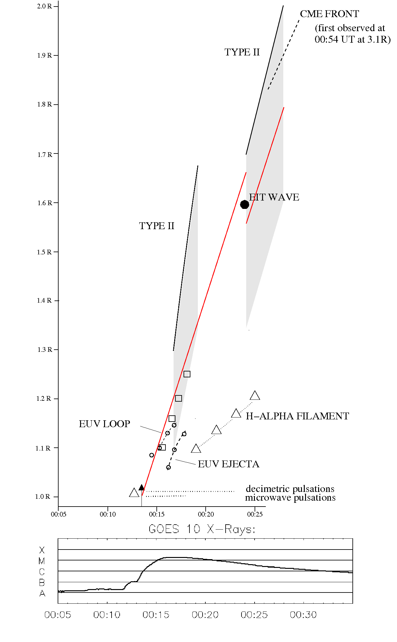
Figure 5.: Estimated (projected) distances of the rising EUV loop and ejecta (circles), H$\alpha$ Moreton wave (boxes), EIT wave (visible at 00:24 UT, but no wave detected in the previous image at 00:12 UT), backward-extrapolated CME front locations, and estimated heights for the type II bursts using a 2 $\times$ Newkirk density model (solid black lines). The shaded areas for the type IIs represent height values that can be obtained with less-dense atmospheric density models. The lower limits are when using the basic Saito density model (see text for details). Red lines give the height–time trajectories for a disturbance traveling at a speed of 725 km s^-1 and appearing at a height of 1.2 $R_{\odot}$ at 00:16:40 UT and at a height of 1.55 $R_{\odot}$ at 00:24 UT (calculated from the frequency drifts and scale heights). The time periods for the microwave and decimetric pulsations are indicated with dotted lines, and black arrow marks the start time of the drifting continuum emission near 1 GHz. Triangles indicate the start time of the filament eruption and the estimated later heights obtained from the H$\alpha$ observations. The GOES soft X-ray flux curve at 3 – 25 keV is shown at the bottom.

Figure 5 summarizes the height versus time relations for the metric type II bursts. Height ranges are shown from the basic Saito and two-times Newkirk atmospheric models. Figure 5 also shows the height–time trajectory for a disturbance traveling at 725 km s^-1, passing the height of 1.2 $R_{\odot}$ at the time of the first type II burst appearance. A disturbance propagating at the same speed would have to be located at a lower height at the time of the second type II burst. The projected distances for the EUV loop front, EUV ejecta, Moreton wave, apparent front of the ejected H$\alpha$ filament, EIT wave, and the backward-extrapolated CME front are also given. In the plot, the time periods of radio pulsations, start time of the drifting continuum emission, and the GOES soft X-ray flux are shown for reference.

To analyze the drifting continuum emission we cannot calculate height estimates, since the frequency drifts can indicate both expanding volume (decreasing density within the volume) and/or rising structures (decreasing atmospheric density). We compared the HiRAS dynamic spectrum with the six NoRP single-frequency observations at 1, 2, 3.75, 9.4, 17, and 35 GHz. We interpolated the radio intensity over 1 – 100 GHz using a least squares fit for the six frequencies. The interpolated data suggest a possible expansion front – defined here as the leading front or border of a fast-expanding structure – and visible as the leading edge of the continuum emission (Figure 6). This leading edge is marked with stars in the plot. Electrons may have been trapped in, for example, an expanding solar magnetic arch and emitted gyrosynchrotron radiation. The continuum could then reveal radiation from nonthermal electrons confined within the plasma volume, which drives a shock. An expansion front would be located at the outer boundary of the expanding volume, and the shock would be located ahead of it. The distance between the driver and the shock is discussed more in Section 4.

The continuum appeared at about the time of the filament eruption, at 00:13 UT, which is almost two minutes before eruption or shock signatures at other wavelengths were observed. The computed kinematics presented by grechnev08 for the Moreton and EIT waves, also suggest that the waves were formed later, around 00:15 UT.

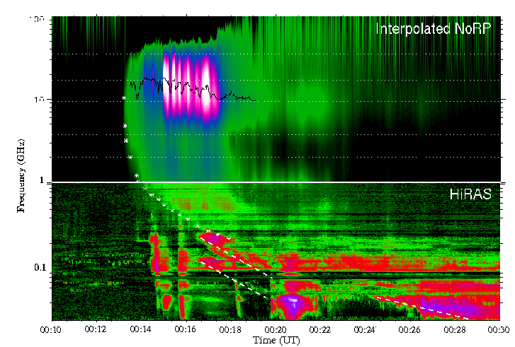
Figure 6.: Interpolation of NoRP single-frequency observations above 1 GHz (with the dotted horizontal lines showing the observing frequencies) combined with the HiRAS dynamic spectral data. The plot shows a possible expansion front (marked with stars), which can be associated with the CME and the type II bursts. The first type II burst (with fundamental and second harmonic emission lanes indicated with dashed lines) appears in a region with lower electron density/lower plasma frequency), and the later second type II burst (with only one emission lane marked here) falls approximately within the drifting continuum. Emission at microwaves show quasi-periodic pulsations (not discussed in this paper).

4 Results and Discussion

We can summarize the multi-wavelength analysis of the 13 July 2004 event with the following results:

1. The event started with a filament eruption, followed closely by the appearance of a frequency-drifting radio continuum. The constructed microwave–meterwave dynamic spectrum (Figure 6) suggests that an expansion front was formed at the time of the filament eruption, almost two minutes prior to any signatures of shock wave formation at other wavelengths. This expanding plasma volume could have been driving a shock wave.

2. The first type II burst was observed in the dynamic spectrum soon after the EUV ejecta lifted off (from below the EUV loop system) and the Moreton wave appeared. The estimated type II burst velocity is similar to the Moreton wave velocity ($\approx$ 700 km s^-1), if the type II burst source height is set untypically low, $\lesssim$ 0.2 $R_{\odot}$ above the photosphere. The type II burst heights then match with the projected distances of the Moreton wave front. We do not expect the Moreton wave and type II burst speeds to be exactly the same. According to Uchida’s model Uchida (1974), the H$\alpha$ Moreton wave is created when the "skirt" of a shock wave sweeps the chromosphere. The shock velocity upward probably differs from the horizontal velocity, but the observed velocities can still be used as rough estimates for the shock speed (like the type II speeds). The backward-extrapolation of a shock propagating with a constant speed of 725 km s^-1 suggests a common start time with the frequency-drifting radio continuum (Figure 5). For comparison, at more typical type II heights, $\approx$ 0.3 – 0.4 $R_{\odot}$, the calculated burst velocities get much higher, $\approx$ 1 000 – 1 700 km s^-1, and no correlation with the heights of other features can be found.

3. The second type II burst had a frequency drift that suggests a speed different from that of the first type II burst, thus implying a different driver for the shock. Calculations show that the type II bursts could have been formed by one shock only, if the shock propagated at a constant speed and the later shocked region was located lower in the shock driver structure (e.g., if the first type II burst was created at the nose of expanding loops and the second one on the sides). The estimated height separation, $\approx$ 0.1 $R_{\odot}$, is not large enough to indicate a separation between, for example, a shock in front of a CME and at the flanks. A decelerating shock would not have been able to produce the observed frequency drift of the second type II burst. A single shock propagating through regions with very different densities, such as first through low density structures and later through high-density streamer regions, would also produce similar jumps in the type II source heights. Despite these different interpretations, the estimated heights for the second type II burst are close to the observed EIT wave distance and the backward-extrapolated CME front distances, although the speeds differ considerably.

Freely propagating shock waves can be formed in flare blasts or when a piston is stopped or it slows down (e.g., vrsnak01). The speed of the propagating shock and the speed of the initial driver can then differ considerably. Also the shock should be spatially well separated from the driver. (In CME-driven shocks observed near Earth, the standoff distance between the shock and its driver has grown to 20 – 50 R_⊙, see Reiner et al., 2007). pomoell08 have shown in their simulations how the speed of the shock (and hence the corresponding type II burst speed) can far exceed the speed of the driver, and the shock can continue propagation through the corona even if the driver speed falls below the local magnetosonic speed. Recent radio imaging observations Dauphin, Vilmer, and Krucker (2006) show a type II burst located ahead of a rising soft X-ray loop. The speed of the rising loop was only 650 km s^-1 at the start time of the type II burst. As stated in their paper, and in another paper analyzing the same event Vrs̆nak et al. (2006), the derived speeds for the type II shocks (obtained with different methods, but in the range of 1 100 – 1 800 km s^-1) are much higher than those of their assumed drivers.

Based on the theory and our calculations for burst heights and speeds, and the observation of the Moreton wave, it is possible that the first type II burst was formed by a blast wave. The earlier start of the frequency-drifting radio continuum suggests that a shock wave may also have been ignited by a fast-expanding structure. Loop-like fronts, such as the rising EUV loop in this case, can be the low-coronal signatures of CMEs Rust and Hildner (1976); Vrs̆nak et al. (2004); Temmer et al. (2008), that drive the shock. gary84 presented a case where a shock is driven by rising loops and a type II burst is due to a flare blast that starts later. In this scenario the type II burst source is located within the ejecta material. Type II emission can also be produced when a flare shock overtakes regions of principal density pile-up near the base and sides of an expanding transient Wagner and MacQueen (1983). This could also explain our low radio source heights.

subra06 have analyzed statistically several doublet type II bursts, and concluded that usually the second type II burst starts at a lower frequency than the first one and the drift rate is only about half of the first one. In our event the frequency drift of the second type II burst is slower by a factor of 4. The rare imaging observations of multiple type II bursts Robinson and Sheridan (1982) suggest that a single shock may exist, but as the shock propagates at different locations the type II bursts may have different characteristics. To verify this, imaging observations are needed at radio and other wavelengths, to determine source locations and corresponding electron densities.

We have presented analysis of a very complex flare-CME event, with a multitude of radio features and transients at other wavelengths, and obtained evidence for both blast wave shock and CME-related emissions during the initial phase. However, definite conclusions will rely on future radio imaging. It is unfortunate that radio imaging currently exists only at very narrow frequency ranges, leaving out plasma emission above 500 MHz and below 150 MHz. For the identification of the source locations in decimetric–metric radio emission, future radio imaging instruments such as the Frequency-Agile Solar Radiotelescope (FASR) will be needed, together with high-cadence multi-wavelength observations. Statistical analyses with comparison to eruption characteristics could also clarify the processes involved.

We wish to thank K-L. Klein for discussions on the use of coronal density models and Victor Grechnev for additional information and discussions on the analysed event. The anonymous referees and Guest Editor K-L. Klein are thanked for valuable comments and suggestions on how to improve the paper. The Global High Resolution H$\alpha$ Network is operated by the Big Bear Solar Observatory, New Jersey Institute of Technology, and we are grateful to V. Yurchyshyn for providing the H$\alpha$ data. We have used in this study radio observations obtained from the Hiraiso Solar Observatory (National Institute of Information and Communications Technology) and Nobeyama Solar Radio Obsevatory (National Astronomical Observatory of Japan), and we thank their staff for making the data available. Wind WAVES data can be obtained from their web archive. SOHO is a project of international cooperation between ESA and NASA. The SOHO LASCO CME Catalog is generated and maintained at the CDAW Data Center by NASA and the Catholic University of America in cooperation with the Naval Research Laboratory. We are grateful to the TRACE, SOHO EIT, LASCO, and MDI teams for making the data available at their Web archives. S.P. and K.H. acknowledge travel grants for this work from the Academy of Finland Project No. 104329.

References

- Brueckner et al. (1995) Brueckner, G.E., Howard, R.A., Koomen, M.J., Korendyke, C.M., Michels, D.J., Moses, J.D., et al.: 1995, Solar Phys. 162, 357.
- Cairns et al. (2003) Cairns, I.H., Knock, S.A., Robinson, P.A., Kuncic, Z.: 2003, Space Sci. Rev. 107, 27.
- Cane and Erickson (2005) Cane, H.V., Erickson, W.C.: 2005, Astrophys. J. 623, 1180.
- Dauphin, Vilmer, and Krucker (2006) Dauphin, C., Vilmer, N., Krucker, S.: 2006, Astron. Astrophys. 455, 339.
- Delaboudinière et al. (1995) Delaboudinière, J.-P., Artzner, G.E., Brunaud, J., Gabriel, A.H., Hochedez, J.F., Millier, F., et al.: 1995, Solar Phys. 162, 291.
- Démoulin and Klein (2000) Démoulin, P., Klein, K.-L.: 2000, in J.-P. Rozelot, L. Klein, J.-C. Vial (Eds.): Transport and Energy Conversion in the Heliosphere, Lecture Notes in Physics 553, 99.
- Dulk (1985) Dulk, G.A.: 1985, Ann. Rev. Astron. Astrophys. 23, 169.
- Gary et al. (1984) Gary, D.E., Dulk, G.A., House, L., Illing, R., Sawyer, C., Wagner, W.J., et al.: 1984, Astron. Astrophys. 134, 222.
- Grechnev et al. (2008) Grechnev, V.V., Uralov, A.M., Slemzin, V.A., Chertok, I.M., Kuzmenko, I.V., Shibasaki, K.: 2008, Solar Phys., in press, DOI 10.1007/s11207-008-9178-8.
- Handy et al. (1999) Handy, B.N., Acton, L.W., Kankelborg, C.C., Wolfson, C.J., Akin, D.J., Bruner, M.E., et al.: 1999, Solar Phys. 187, 229.
- Koutchmy (1994) Koutchmy, S.: 1994, Adv. Space Res. 14, (4)29.
- Klassen, Pohjolainen, and Klein (2003) Klassen, A., Pohjolainen, S., Klein, K.-L.: 2003, Solar Phys. 218 197.
- Klassen et al. (1999) Klassen, A., Aurass, H., Klein, K.-L., Hofmann, A., Mann, G.: 1999, Astron. Astrophys. 343, 287.
- Kundu (1965) Kundu, M.R.: 1965, Solar Radio Astronomy, Interscience.
- Lehtinen et al. (2008) Lehtinen, N.J., Pohjolainen, S., Huttunen-Heikinmaa, K., Vainio, R., Valtonen, E., Hillaris, A.E.: 2008, Solar Phys. 247, 151.
- Lin, Mancuso, and Vourlidas (2006) Lin, J., Mancuso, S., Vourlidas, A.: 2006, Astrophys. J. 649, 1110.
- Lin et al. (2002) Lin, R.P., Dennis, B.R., Hurford, G.J., Smith, D.M., Zehnder, A., Harvey, P.R., et al.: 2002, Solar Phys. 210, 3.
- Mancuso (2007) Mancuso, S: 2007, Astron. Astrophys. 463, 1137.
- Mancuso and Raymond (2004) Mancuso, S., Raymond, J.C.: 2004, Astron. Astrophys. 413, 363.
- Mann, Classen, and Aurass (1995) Mann, G., Classen, T., Aurass, H.: 1995, Astron. Astrophys. 295, 775.
- Mann et al. (2003) Mann, G., Klassen, A., Aurass, H., Classen H.-T.: 2003, Astron. Astrophys. 400, 329.
- Melrose (1980) Melrose, D.B.: 1980, Space Sci. Rev. 26, 3.
- Nakajima et al. (1985) Nakajima, H., Sekiguchi, H., Sawa, M., Kai, K., Kawashima, S.: 1985, Pub. Astron. Soc. Japan 37, 163.
- Nakajima et al. (1994) Nakajima H., Nishio M., Enome S., Shibasaki, K., Takano T., Hanaoka, Y., et al.: 1994, Proc. IEEE 82, 705.
- Nelson and Melrose (1985) Nelson, G.J., Melrose, D.B.: 1985, in Solar Radiophysics, D.J. McLean and N.R. Labrum (eds.), Cambridge Univ. Press, 333.
- Newkirk (1961) Newkirk, G.Jr.: 1961, Astrophys. J. 133, 983.
- Pohjolainen et al. (2007) Pohjolainen, S., van Driel-Gesztelyi, L., Culhane, L., Manoharan, P.K., Elliott, H.A.: 2007, Solar Phys. 244, 167.
- Pomoell, Vainio, and Kissmann (2008) Pomoell, J., Vainio, R., Kissmann, R.: 2008, Solar Phys., in press, DOI 10.1007/s11207-008-9186-8.
- Reiner et al. (2000) Reiner, M.J., Karlický, M., Jiika, K., Aurass, H., Mann, G., Kaiser, M.L.: 2000, Astrophys. J. 530, 1049.
- Reiner, Kaiser, and Bougeret (2007) Reiner, M.J., Kaiser, M.L., Bougeret, J.-L.: 2007, Astrophys. J. 663, 1369.
- Robinson and Sheridan (1982) Robinson, R.D., Sheridan, K.V.: 1982, Proc. ASA 4, 392.
- Rust and Hildner (1976) Rust, D.M., Hildner, E.: 1976, Solar Phys., 48, 381.
- Saito (1970) Saito, K.: 1970, Ann. Tokyo Astr. Obs. 12, 53.
- Subramanian and Ebenezer (2006) Subramanian, K.R., Ebenezer, E.: 2006, Astron. Astrophys. 451, 683.
- Temmer et al. (2008) Temmer, M., Veronig, A.M., Vrs̆nak, B., Rybák, J., Gömöry, P., Stoiser, S., Maric̆ić, D.: 2008, Astrophys. J. 673, L95.
- Thompson et al. (1999) Thompson, B.J., Gurman, J.B., Neupert, W.M., Newmark, J.S., Delaboudiniére, J.-P., St. Cyr, O.C. et al.: 1999, Astrophys. J. 517, L151.
- Uchida (1974) Uchida, Y: 1974, Solar Phys., 39, 431.
- Vrs̆nak (2001) Vrs̆nak, B.: 2001, J. Geophys. Res. 106, 25291.
- Vrs̆nak (2005) Vrs̆nak, B.: 2005, EOS Transactions 86, 112.
- (40) Vrs̆nak, B., Magdalenic̆, J., Zlobec, P.: 2004, Astron. Astrophys. 413, 753.
- Vrs̆nak et al. (2004) Vrs̆nak, B.; Maric̆ić, D., Stanger, A.L., Veronig, A.: 2004, Solar Phys., 225, 355.
- Vrs̆nak et al. (2006) Vrs̆nak, B., Warmuth, A., Temmer, Veronig, A., Magdalenic̆, J., Hillaris, A., Karlicky, M.: 2006, Astron. Astrophys. 448, 739.
- Wagner and MacQueen (1983) Wagner, W.J., MacQueen, R.M.: 1983, Astron. Astrophys. 120, 136.
- Warmuth (2007) Warmuth, A. 2007, in The High Energy Solar Corona: Waves, Eruptions, Particles, ed. K.-L. Klein, A.L. MacKinnon, Lect. Notes Phys. 725, Springer, 107.
- Warmuth and Mann (2005) Warmuth, A., Mann, G.: 2005, Astron. Astrophys. 435, 1123.