Soft processes at high energy without soft Pomeron:
a QCD motivated model.

Abstract:

In this paper we develop a QCD motivated model for both hard and soft interactions at high energies. In this model the long distance behavior of the scattering amplitude is determined by the approximate solution to the non-linear evolution equation for parton system in the saturation domain. All phenomenological parameters for dipole-proton interaction were fitted from the deep inelastic scattering data and the soft processes are described with only one new parameter, related to the wave function of hadron. It turns out that we do not need to introduce the so called soft Pomeron that has been used in high energy phenomenology for four decades. The model described all data on soft interactions: the values of total, elastic and diffractive cross sections as well as their $s$ and $t$ behavior. The value for the survival probability of the diffractive Higgs production is calculated being less 1% for the LHC energy range.

1 Introduction

For three decades our microscopic theory-QCD, has been unable to describe soft (long distance) interactions. It happens, partly, because of the embryonic stage of our understanding of the most challenging problem in QCD: confinement of quarks and gluons. We believe, however, that the main features of high energy scattering at long distances can be described in the framework of QCD, and such a description is based on the phenomenon of saturation of the parton densities in QCD [1, 2, 3]. Indeed, at short distances the parton densities increase with the growth of energy due to gluon emission, which is described by the QCD linear evolution equations [4, 5]. Such an emission is proportional to the density of emitters (partons). The process of annihilation is suppressed since it’s strength is proportional to the parton density squared, reflecting the fact that two partons have to meet each other in the small volume of interaction. However, at high energy the density of partons becomes so large that the annihilation term tends to be of the same order as the emission term. It leads to a slow down in the increase of the parton density, and the system of partons lives in the dynamical equilibrium with the critical value of density (it is saturated). We have several theoretical approaches for a QCD description of the parton system in the saturation domain (see Ref. [1, 2, 3, 6, 7, 8, 9, 10, 11, 12], but the equations that have been proposed turn out to be so complicated, that our knowledge about this domain mostly stems from numerical solutions of these equations [13].

The alternative approach that has been developed during the past decade is to build models [14, 15] that incorporate the main qualitative properties of these solutions, such as the geometrical scaling behavior of the scattering amplitude [19, 20, 21] and the existence of the new dimensional scale (the so called saturation scale) [1, 2, 3], which increases in the region of low $x$ (high energy). Such models successfully described all the data on deep inelastic scattering, including the behavior of inclusive and diffractive cross sections, at a low value of photon virtuality [14].

The main goal of this paper is to describe the processes that occur at long distances (soft processes), where we cannot apply perturbative QCD, using the saturation model. In this model all the needed phenomenological parameters, in particular the energy behavior and the value of the saturation scale, were fitted using the DIS data. The main ingredient of the high energy phenomenology during the past four decades, namely the soft Pomeron, is not introduced in this model. In simple words, we replace the soft Pomeron by the scattering amplitude that describes the behavior of the saturated parton system. The idea, that the matching between soft and hard interaction occurs in the saturation region, and can be described by the amplitude that originates from the high density QCD approach, is not new. This idea has been in the air for a number of years and have been advocated in several lectures on the subject [22]. The first attempt of a practical application of this idea was done in Ref. [24] (see also Ref. [25]). The result of this paper was encouraging since the estimates gave a reasonably good agreement with the experimental data on the total cross section of the pion, kaon, and proton interaction with the proton target. In this paper we continue to develop these ideas and we give the comparison with the experiment data for the full set of the experimental data of soft interactions, that include the energy behavior of the total, elastic and diffraction cross sections as well as a $t$- behavior of the elastic cross sections, and the mass behavior for the cross sections of diffraction production.

2 The main idea

As has been mentioned, our main idea is to describe the so called ‘soft’ interaction in the high parton density QCD (hdQCD). In hdQCD we are dealing with the dense system of partons which cannot be treated in the perturbative QCD approach. Being non-perturbative in its nature, hdQCD leads to typical distances $r=1/Q_{s}(x)\ll R\sim 1/\Lambda_{QCD}$ where $R$ is the size of a hadron. The saturation momentum $Q_{s}(x)$ is a new dimensionful scale which increases with the growth of the energy ( or at $x\to 0$)[1, 2, 3]. Therefore, the QCD coupling $\alpha_{S}\left(Q_{s}(x)\right)$ is small and, because of this, we are able to develop a theoretical approach for such a dense system having only a limited input from the unknown confinement region. To illustrate the limitation of our approach, it is enough to look at the expression for the saturation scale in hdQCD[1, 26]

$$Q^{2}_{s}(Y)\,\, = \,\,Q^{2}_{s}(Y_{0})\,\exp\left(\bar{\alpha}_{S}\,\frac{\chi(\gamma_{cr})}{1-\gamma_{cr}}\,\,(Y-Y_{0})\,\,-\,\,\frac{3}{2(1-\gamma_{cr})}\,\ln(Y/Y_{0})-\right.$$

$$- \,\left.\frac{3}{(1-\gamma_{cr})^{2}}\,\sqrt{\frac{2\,\pi}{\bar{\alpha}_{S}\,\chi^{\prime\prime}(\gamma_{cr})}}\,(\frac{1}{\sqrt{Y}}\,-\,\frac{1}{\sqrt{Y_{0}}}\,)\,,+\,O(\frac{1}{Y})\right)$$ (2.1)

In Eq. (2) the energy dependence of $Q_{s}(Y=\ln(1/x))$ is predicted from hdQCD, ($\chi(\gamma)$ is the Mellin transform of the BFKL kernel) but the scale $,Q^{2}_{s}(Y_{0})$ stems from the confinement region, demonstrating a need for some input from this theoretically unknown region. Our hope that such input will be a limited number of constants.

Let us consider the deep inelastic electron-proton scattering (DIS), to illustrate our point. If the virtuality of the photon $Q^{2}$ is very large, $Q^{2}\gg Q^{2}_{s}(x)$, the typical distances $r\approx 1/Q$, and we can safely apply the perturbative QCD approach based on the operator product expansion, and the DGLAP evolution equation. However, if $\Lambda^{2}_{QCD}\ll Q^{2}\ll Q^{2}_{s}(x)$, the situation changes crucially. All terms in the operator product expansion become of the same order, and we have to use the hdQCD approach. In this approach, the cross section $\sigma^{\gamma^{*}p}$ shows a geometrical scaling behaviour[27], namely, $\sigma^{\gamma^{*}p}=\left(1/Q^{2}_{s}(x)\right)\,F\left(Q^{2}/Q^{2}_{s}(x)\right)$ which has been confirmed experimentally. This means that the typical distances $r\approx 1/Q_{s}(x)\ll 1/\Lambda_{QCD}$, which are short.

Our idea is that we can describe $Q^{2}\approx\Lambda^{2}_{QCD}$, in the framework of the same hdQCD approach. Having the geometrical scaling behavior in mind, such an idea does not look crazy. However, in DIS we are dealing with the total cross sections which are related to the amplitude integrated over the impact parameters ($b$). For a treatment of the soft interaction observables, we need to know the $b$ dependence. As was shown in Ref. [28], hdQCD predicts the power-like decrease at large value of $b$, which contradicts both the theoretical estimates and experimental observations. Therefore, we need an input from the confinement region to specify the $b$ dependence of the scattering amplitude. Let us first discuss large $b\geq 1/\Lambda_{QCD}\gg 1/Q_{s}(x)$. The scattering amplitude for DIS $A\left(Q^{2},W;t\right)$ depends on the photon virtuality $Q^{2}$, energy $W=\sqrt{s}=Q/\sqrt{x}$ and on the momentum transferred $t=-q^{2}<0$. Using the dispersion relation in the $t$-channel we have

$$A\left(Q^{2},W;t\right)\,\,=\,\,\frac{1}{\pi}\,\int^{\infty}_{4m^{2}_{\pi}}\,\frac{dt^{\prime}\,Im_{t}A\left(Q^{2},W;t^{\prime}\right)}{t^{\prime}+q^{2}}$$ (2.2)

Calculating the amplitude in the impact parameter representation we can reduce Eq. (2.2) to the form

$$A\left(Q^{2},W;b\right)\,\, = \,\,\frac{1}{(2\pi)^{2}}\,\int\,d^{2}\vec{q}\,A\left(Q^{2},W;t\right)\,e^{i\vec{q}\cdot\vec{b}}\,\,=\,\,\frac{1}{2\pi^{2}}\,\int^{\infty}_{4m^{2}_{\pi}}\,dt^{\prime}\,Im_{t}A\left(Q^{2},W;t^{\prime}\right)\,\int\,\frac{q\,dq\,\,J_{0}\left(qb\right)}{t^{\prime}+q^{2}}\,$$

$$= \,\,\frac{1}{2\pi^{2}}\,\int^{\infty}_{4m^{2}_{\pi}}\,dt^{\prime}\,K_{0}\left(\sqrt{t^{\prime}}\,b\right)\,\,Im_{t}A\left(Q^{2},W;t^{\prime}\right)\,\,\ \stackrel{{\scriptstyle b\geq 1/(2m_{\pi})}}{{\longrightarrow}}\,C\,Im_{t}A\left(Q^{2},W;t^{\prime}=4m^{2}_{\pi}\right)\,K_{0}\left(2m_{\pi}b\right)$$

where in the constant $C$, all the numerical factors have been absorbed.

In Eq. (2), the $b$-dependence is determined by the mass of the lightest hadron (pion), and cannot not be reproduced in perturbative or/and high density QCD. However, one can see from Eq. (2) that we have a factorization of the $b$ dependence, and the dependence on the photon virtuality and energy.

As it is well known (see Ref. [12] and references therein), in the kinematic region $\alpha_{S}\,\leq\alpha_{S}\,\ln(1/x)\leq 1/\alpha_{S}$ in the saturation region the hdQCD approach reduces to the BFKL Pomeron calculus. We generalize Eq. (2) for the BFKL Pomeron in the following way

$$A_{BFKL}\left(Q^{2},x;b\right)\,\,\,=\,\,\,\stackrel{{\scriptstyle\mbox{ \small short distances}}}{{A_{BFKL}\left(Q^{2},x;t=0\right)}}\,\times\,\stackrel{{\scriptstyle\mbox{\small long distances}}}{{S(b)}}$$ (2.4)

One can see that Eq. (2.4) claims a kind of factorization between short and long distances. The short distance part we can describe in hdQCD, while the long distance part has to be taken from the confinement domain. In a more general way, we can re-write Eq. (2.4) in the form

$$A_{BFKL}\left(Q^{2},x;\vec{b}\right)\,\,\,=\,\,\,\int d^{2}\vec{b^{\prime}}\stackrel{{\scriptstyle\mbox{ \small short distances}}}{{A_{BFKL}\left(Q^{2},x;\vec{b^{\prime}}\right)}}\,\times\,\stackrel{{\scriptstyle\mbox{\small long distances}}}{{S(\vec{b}-\vec{b}^{\prime})}}$$ (2.5)

where $b^{\prime}$ in the short distance part is of the order of $b^{\prime}\approx 1/Q_{s}(x)$.

The approach of Eq. (2.4) and Eq. (2.5), at first sight contradicts the high energy phenomenology based on the soft Pomeron and Reggeons, as well as well as the lattice calculations [30]. In both approaches, the Pomeron trajectory has $\alpha^{\prime}_{{I\!\!P}}>0$, and at positive $t$ the glueballs lie on this trajectory. In Eq. (2.4) and Eq. (2.5), the Pomeron slope $\alpha^{\prime}_{{I\!\!P}}=0$. We will show below that we will be able reproduce the experimental data on energy dependence of the elastic slope which used to consider as the argument for $\alpha^{\prime}_{{I\!\!P}}=0.25\,GeV^{-2}$. On the theoretical side, the only theory which can treat at the moment on the same footing both short and long distances: N=4 SYM with AdS/CFT correspondence, leads to a picture which is in striking agreement with our approach[29]. Namely, in this approach at $t>0$ ( resonance region) we have a normal soft Pomeron with $\alpha^{\prime}_{{I\!\!P}}>0$ while at $t<0$ (scattering region) $\alpha^{\prime}_{{I\!\!P}}=0$.

3 The model

3.1 Motivation

Our building of the model is based on the dipole approach to high energy QCD [31]. In this approach, the evolution of the parton (colorless dipole) system can be written in the form of the equation for the generating functional, with a transparent probabilistic interpretation for them. The generating functional is defined as [31]

$$Z\left(Y\,-\,Y_{0};\,[u]\right)\,\,\equiv\,\,\sum_{n=1}\,\int\,\,P_{n}\left(Y\,-\,Y_{0};\,x_{1},y_{1};\dots;x_{i},y_{i};\dots;x_{n},y_{n}\right)\,\,\prod^{n}_{i=1}\,u(x_{i},y_{i})\,d^{2}\,x_{i}\,d^{2}\,y_{i}$$ (3.6)

where $u(x_{i},y_{i})\equiv u_{i}$ is an arbitrary function of $x_{i}$ and $y_{i}$. The coordinates $(x_{i},y_{i})$ describe the colorless pair of gluons or a dipole. $P_{n}$ is a probability density to find $n$ dipoles with the size $x_{i}-y_{i}$, and with impact parameter $(x_{i}+y_{i})/2$. Assuming that we have only a decay of one dipole to two dipoles, directly from the physical meaning of $P_{n}$ it follows [31, 32, 33]

$$\frac{\partial\,P_{n}(Y;\dots;x_{i},y_{i};\dots;x_{n},y_{n})}{\partial Y}\,\,\,=$$ (3.7)

$$=\,\,\sum_{i}\ V_{1\to 2}\bigotimes\left(P_{n-1}(Y;\dots;x_{i},y_{i};\dots;x_{n},y_{n})\,-\,P_{n}(Y;\dots;x_{i},y_{i};\dots;x_{n},y_{n})\right)$$

where $\bigotimes$ denotes all necessary integrations and $V_{1\to 2}$ is the vertex for the decay of one dipole to two dipoles. This vertex is equal to

$$V_{1\to 2}\left((x,y)\to(x,z)+(z,y)\right)\,\,=\,\,\frac{\bar{\alpha}_{S}}{2\pi}\,\frac{(\vec{x}-\vec{y})^{2}}{(\vec{x}-\vec{z})^{2}\,(\vec{z}-\vec{y})^{2}}$$ (3.8)

Eq. (3.7) is a typical Markov’s chain which takes into account the $s$ - channel unitarity on each step of evolution since it has two terms: the birth of the new dipole due to the decay of the parent dipole (positive term in Eq. (3.7)) and the death of the dipole due to the same process.

Eq. (3.7) can be rewritten as the equation for the generating functional [32, 33], namely,

$$\frac{\partial\,Z\,\left(Y-Y_{0};[\,u\,]\right)}{\partial\,Y}\,\,=\,\,\int\,d^{2}x\,d^{2}y\,d^{2}z\,\,V_{1\to 2}\left((x,y)\to(x,z)+(z,y)\right)\,\frac{\partial}{\partial\,u(x,y)}\,\,Z\,\left(Y-Y_{0};[\,u\,]\right)$$ (3.9)

$Z\,\left(Y-Y_{0};[\,u\,]\right)$ satisfies the initial and boundary conditions:

Initial         conditions: $$Z\,\left(Y-Y_{0}=0;[\,u\,]\right) =\,\,\,u(x,y)\,;$$ (3.10)

Boundary conditions: $$Z\,\left(Y-Y_{0};[\,u=1\,]\right) =\,\,\,1\,;$$ (3.11)

The advantage of the generating functional is that we can write it in terms of this simple functional formulae for the scattering amplitude, which has an obvious partonic interpretation. Indeed, the scattering amplitude in the lab. frame can be written in the form [6, 32, 33]

$$N\left(Y-Y_{0};r,b\right)\,\,=$$ (3.12)

$$\,\,\sum^{\infty}_{n=1}\,\frac{(-1)^{n}}{n!}\,\,\int\,\prod^{n}_{i=1}\,\,d^{2}\,x_{i}\,d^{2}\,y_{i}\,\,\rho_{n}\left(r,b;\{x_{i},y_{i}\},Y-Y_{0}\right)\gamma_{n}\left(r,b;\{x_{i},y_{i}\},Y_{0}\right)$$

where $Y-Y_{0}\,\,\gg\,\,1$ but $Y_{0}\,\,\approx\,\,1$ and

$$\rho_{n}\left(Y-Y_{0},\{x_{i},y_{i}\}\right)\,\,\,=\,\,\,\prod^{n}_{i=1}\,\frac{\delta}{\delta u(x_{i},y_{i})}Z\,\left(Y-Y_{0};\{\,u(x_{i},y_{i})\,\}\right)|_{u(x_{i},y_{i})=1}$$ (3.13)

and $\gamma_{n}$ is the amplitude of interaction of $n$ dipoles at low energy ( small values of rapidity $Y_{0}$) with the coordinates $x_{i},y_{i}$ with the target with size $r$ and impact parameter $b$. In the parton language the generating functional determines the parton wave function for which we have the evolution equation Eq. (3.9) in QCD. $\gamma_{n}$ can have a non-perturbative origin. We assume that $\gamma_{n}\left(r,b;\{x_{i},y_{i}\},Y_{0}\right)\,\,=\,\,\prod^{n}_{i=1}\gamma(x_{i},y_{i};Y_{0})$. This assumption means that the dipoles inside the target have no correlation, which is correct, as far as we know, only for a nucleus target.

In spite of the transparent physics behind our equations, the equation for the generating functional is difficult to solve analytically, especially if we generalize Eq. (3.9) to the case of the so called Pomeron loops [35, 36, 37]. As has been mentioned, we wish to find a model solution to Eq. (3.9). We will do this using two key observations of Ref.[12]. The first one is the fact that in the huge kinematic region of $\bar{\alpha}_{S}Y\,\leq 1/\bar{\alpha}_{S}$, the system of partons that we are dealing with turns out to be a system of non-interactive partons. In other words, it means that the generating functional of Eq. (3.6) can be rewritten in a simpler form, namely.

$$Z\,\left(Y-Y_{0};\{\,u(x_{i},y_{i})\,\}\right)\,\,\,=\,\,\,\sum^{\infty}_{n=1}\,\frac{C_{n}}{n!}\,\,\left(\int\,d^{2}x^{\prime}\,d^{2}y^{\prime}\,P(Y-Y_{0};x,y;x^{\prime},y^{\prime})\,\,\left(u(x^{\prime},y^{\prime})\,-\,1\right)\right)^{n}$$ (3.14)

where $P(Y-Y_{0};x,y;x^{\prime},y^{\prime})$ is the amplitude for one BFKL Pomeron exchange, between dipoles $(x,y)$ and $(x^{\prime},y^{\prime})$.

In Ref.[12] it was shown , using the analytical solution of Ref. [34] , that actually $C_{n}\,=\,1$ for the dipoles with the size $r\sim 1/Q^{2}_{s}$ where $Q_{s}$ is the saturation momentum.

Therefore, Eq. (3.14) can be simplified and rewritten in the form

$$Z\,\left(Y-Y_{0};\{\,u(x_{i},y_{i})\,\}\right)\,\,\,=\,\,\,\exp\left(\int\,d^{2}x^{\prime}\,d^{2}y^{\prime}\,P(Y-Y_{0};x,y;x^{\prime},y^{\prime})\,\left(u(x^{\prime},y^{\prime})\,-\,1\right)\right)$$ (3.15)

and the amplitude has the form

$$N\left(Y-Y_{0};x,y\right)\,\,=\,\,1-\exp\left(-\int\,d^{2}x^{\prime}\,d^{2}y^{\prime}\,\,P\left(Y-Y_{0};x,y;x^{\prime},y^{\prime}\right)\gamma\left(Y_{0};x^{\prime},y^{\prime}\right)\right)$$ (3.16)

where $\gamma\left(Y_{0};x^{\prime},y^{\prime}\right)$ is the scattering amplitude of the dipole $(x^{\prime},y^{\prime})$, with the target at low energy.

3.2 Main formulae and assumptions

Eq. (3.16) is the main formula for constructing our model. The first ingredient of the model is the choice of the amplitude $\gamma$ and the value of $Y_{0}$. We choose this amplitude in the form [38]

$$\gamma\left(Y_{0};x^{\prime},y^{\prime}\right)\,\,=\,\,\gamma_{mod}\left(Y_{0};x^{\prime},y^{\prime}\right)\,\,=\,\,\,\,\frac{\pi^{2}\,\alpha_{S}(\mu^{2})}{3}\,r^{2}\,x_{0}G^{DGLAP}(x_{0},\mu^{2})\,S(b)$$ (3.17)

where $\vec{r}\,=\,\vec{x}-\vec{y}$ and $\vec{b}=\frac{1}{2}\,(\vec{x}+\vec{y})$ with $x_{0}=10^{-2}$. $xG$ in Eq. (3.17) is the solution of the DGLAP evolution equation which describes the DIS experimental data. $\mu$ is equal to

$$\mu^{2}\,\,=\,\,\mu^{2}_{0}\,\,+\,\,\frac{C}{r^{2}}$$ (3.18)

where $\mu_{0}$ and $C$ are phenomenological parameters which has to be found fitting the experimental data on DIS (see Ref.[15] for details). Eq. (3.18) means that $\gamma_{mod}\left(Y_{0};x^{\prime},y^{\prime}\right)$ at large dipole size $r\mu_{0}\gg 1$ is determined by the following expression

$$\gamma_{mod}\left(Y_{0};x^{\prime},y^{\prime}\right)\,\,=\,\,\,\,\frac{\pi^{2}\,\alpha_{S}(\mu^{2}_{0})}{3}\,r^{2}\,x_{0}G^{DGLAP}(x_{0},\mu^{2}_{0})\,S(b)$$ (3.19)

Of course Eq. (3.19) has no theoretical basis, and our hope is that the amplitude at low $x$ will be not very sensitive to this kinematic region, in the initial condition.

$S(b)$ is the impact parameter profile function, which is chosen as the Fourier image of the proton form factor, namely,

$$S(b)\,\,=\,\,\frac{2}{\pi\,R^{2}}\left(\frac{\sqrt{8}\,b}{R}\right)\,K_{1}\left(\frac{\sqrt{8}\,b}{R}\right)$$ (3.20)

where $R$ is the proton radius ($R=0.89\,fm$).

In Eq. (3.16) $P\left(Y-Y_{0};x,y;x^{\prime},y^{\prime}\right)$ stands for the BFKL Pomeron Green’s function. This Green’s function describes the energy ($x$) evolution of the gluon system in the region of high energy (low $x$). This evolution allows us to find the dipole scattering amplitude or parton density at low $x$ from the initial condition: the amplitude at lower $x=x_{0}$, but for any value of the dipole size ($r$).

However, we know that the BFKL Pomeron alone cannot describe the experimental data, since it determines the anomalous dimension only at low $x$. The experimental data shows a good agreement with the DGLAP evolution equation, which is written as the evolution in $\ln(\mu^{2})$ (see Eq. (3.17)), which gives us the parton density from the boundary condition: the parton density at $\mu^{2}=\mu^{2}_{0}$ but at any value of $x$ including the region of low $x$. Strictly speaking, it cannot be used in Eq. (3.16), but assuming Eq. (3.18) for the scale $\mu^{2}$, we impose the condition that at long distances, the typical momentum scale in the linear evolution equation is equal to $\mu^{2}_{0}$. In the framework of this assumption, it looks reasonable to assume that

$$\Omega(Y,r,b)\,\,\, = \,\,2\,\int\,d^{2}x^{\prime}\,d^{2}y^{\prime}\,\,P\left(Y-Y_{0};x,y;x^{\prime},y^{\prime}\right)\gamma\left(Y_{0};x^{\prime},y^{\prime}\right)\,\,$$ (3.21)

$$= \frac{\pi^{2}\,\alpha_{S}(\mu^{2})}{3}\,r^{2}\,xG^{DGLAP}(x,\mu)\,S(b)$$

Finally, we can write the following model expression for the scattering amplitude;

$$N\left(x;r,b\right)\,\,\,=\,\,1\,\,\,-\,\,\exp\left(-\frac{1}{2}\Omega\left(x,r,b\right)\right)$$ (3.22)

where $\Omega\left(x,r,b\right)$ is given by Eq. (3.21).

3.3 Fixing the values of the phenomenological parameters

In Eq. (3.18) we have introduced two phenomenological parameters: $\mu^{2}_{0}$ and $C$. The first determines the value of the virtuality of the probe in DIS processes from which we can start using the perturbative QCD evolution equations. The second ($C$) gives the relation between scales in the momentum representation and in the coordinate representation. In the case of the DGLAP evolution, $C=4$ ( see Ref. [38]), but since the amplitude has a more complicated form than Eq. (3.22), the value of $C$ can be different.

Two more parameters stem from the initial condition for the gluon density in Eq. (3.21), namely,

$$xG^{DGLAP}\left(x,Q_{0}^{2}\right)\,\,\,=\,\,\frac{A}{x^{\omega_{0}}}(1-x)^{6}\,$$ (3.23)

which corresponds to the exchange of the soft Pomeron with the intercept $\omega_{0}$ at the initial hard scale $\mu^{2}=Q^{2}_{0}$ in traditional high energy phenomenology, and the factor $(1-x)^{6}$ reflects the valence quark dependance. In our approach we do not assume that the soft Pomeron exists, and we view Eq. (3.23) just as the simplest function that reflects the behavior of the experimental data in DIS.

We use the observation of Ref. [39], that the anomalous dimension in the leading order can be written in a very simple form, namely,

$$\gamma(\omega)\,\,=\,\,\bar{\alpha}_{S}\left(\frac{1}{\omega}\,\,-\,\,1\right)$$ (3.24)

The explicit solution to the DGLAP evolution equation with $\gamma(\omega)$ of Eq. (3.24), and with the initial condition of Eq. (3.23), has been found in Ref. [15] and looks as follows

$$xG^{DGLAP}(x,t)\,=\,\sum_{k=0}^{6}\binom{6}{k}\,(-1)^{k}\,xG^{(k)}(x,t,\omega_{k})$$ (3.25)

where

$$xG^{(k)}\left(y\equiv\ln(1/x),t,\omega_{k}\right)\,\,=\,\,A\,e^{-t\,+\,\omega_{k}\,y}\,\,\left\{\int^{y}_{0}\,\,dy^{\prime}\,e^{-\omega_{k}\,y^{\prime}}\,\sqrt{\frac{t}{y^{\prime}}}\,\,I_{1}\left(2\sqrt{t\,y^{\prime}}\right)\,\,\,+\,\,\,1\right\}$$ (3.26)

with

$$\omega_{k}=\omega_{0}-k\,;\;\;\;\;t\,\,\,\equiv\,\,\,\frac{4N_{c}}{b_{0}}\,\ln\frac{\ln\left(\mu^{2}/\Lambda^{2}\right)}{\ln\left(\mu^{2}_{0}/\Lambda^{2}\right)}\,;\,\,\,\,\,\,\,\,b_{0}\,\,=\,\,11-\frac{2n_{f}}{3}\,\,\,\,\,\mbox{and}\,\,\,\,\,\,\,\,y\,=\,\ln(1/x)$$ (3.27)

In Eq. (3.21) the typical scale of hardness in the gluon structure function is determined by the process of gluon emission while the factor $\alpha_{S}\,r^{2}$ takes into account the integration over the wave function of the dipole with the size $r$. Having this in mind, we introduce a different scale for $\alpha_{S}$ in Eq. (3.21). Finally, we use

$$\Omega(x,r,b)\,\,\,=\,\,\,\frac{\pi^{2}\,\alpha_{S}(\tilde{\mu}^{2})}{3}\,r^{2}\,xG^{DGLAP}(x,\mu)\,S(b)\,\,\,\mbox{with}\,\,\,\tilde{\mu}^{2}\,\,=\,\,\tilde{\mu}^{2}_{0}\,\,+\,\,\frac{C}{r^{2}}$$ (3.28)

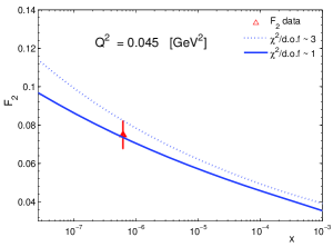
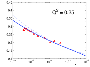
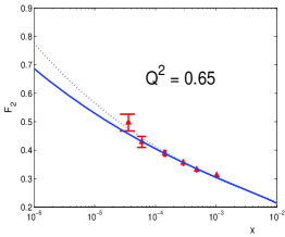
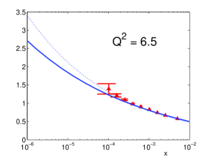
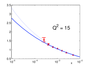
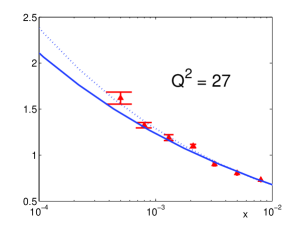
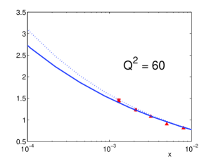
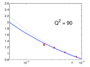
where $xG^{DGLAP}(x,\mu)$ is given by Eq. (3.26) and the initial hard scale $\widetilde{\mu}^{2}_{0}$ is different from that of $\mu_{0}^{2}$. We perform a fit of the saturation model, to the DIS experimental data and fixing the parameters, we wish to describe the soft data without using the concept of the ”soft” pomeron. The fit procedure was performed by using the minuit routine, the statistical and systematical errors have been added in quadrature. We have used all of the recent data on deep inelastic scattering processes, from different collaborations. The most suitable were H1 [16] and ZEUS [17, 18]. It was observed, that H1 data for medium and large values of $Q^{2}$ coincides with that from the ZEUS col., but up to a scaling factor of 1.05. Hence, for the fitting procedure, we took only the ZEUS data for vary small, medium and large values of $Q^{2}$. Since we are interested in the high energy description, we took data below $x<0.01$ and $0.045<Q^{2}<150GeV^{2}$. The upper limit on virtuality is originated from the upper limit on the $x$ variable. Fitting with H1 scaled data, yields almost the same result. The total number of experimental points was 170. During the fitting procedure, we observed a strong correlation between different parameters, so we decided to fix a number of them. We choose to fix a parameter $C$ and the initial hard scale $Q^{2}_{0}$. The masses of the quarks were taken as follows: $m_{light}\;=\;0.25\;GeV$ and $m_{charm}\;=\;1.3\;GeV$. $\chi^{2}$ for this parametrization is $\thicksim 1.05$. The summary of the fitting procedure is given in the table 1

Model	$\widetilde{\mu}_{0}^{2}$	$\mu_{0}^{2}$	$Q_{0}^{2}$	$C$	$\omega_{0}$	$A$	$\chi^{2}/d.o.f.$
A	0.23	1.23	1.0	1.0	0.028	1.81	1.04
B	0.069	1.23	0.58	1.0	0.087	0.6	3.08

Table 1: Resulting parameters from the fit to DIS data Model A gives a very good description of the DIS data, while model B reproduces quite well the data on soft processes.

The bolded font corresponds to the fixed parameters $C$ and $Q^{2}_{0}$, which were chooses to be equal to $1.0$. The value of the hard scale $\mu^{2}_{0},\;\widetilde{\mu}_{0}^{2}$. is in the units of energy $GeV$.

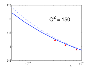
As one can see, $\chi^{2}/d.o.f.$ is close to 1 and fit gives very good description of all experimental data on DIS (see Fig. 1). However, we present in Table 1 a second fit which leads to worse $\chi^{2}/d.o.f.$ but reproduces the data on soft interaction quite well as we will see below. It should be stressed that both fits describe the DIS data at large values of photon virtualities with small $\chi^{2}/d.o.f.$ . Therefore, we can consider model the A as an attempt to describe the experimental data on DIS and soft processes, assuming that Eq. (3.22) is correct in the saturation region. In model B we explore a different idea: Eq. (3.22) is only approximate formula that incorporates the main qualitative properties of scattering amplitude for both DIS and soft scattering in the saturation region. The question which we try to answer using model B is the following: is it possible to give the unique description of long distance physics both in DIS and soft interaction based on the QCD amplitudes at short distances.

Figure 1: Description of the DIS experimental data in our models. Dotted line describes the model B while solid line corresponds to Model A.

4 Cross sections of hadron-hadron interaction at high energy

4.1 General approach

Eq. (3.22) gives a smooth continuation to the long distance physics describing the DIS data at very low values of the photon virtualities. We wish to extend this description to the hadron-hadron interaction without assuming something in addition, for example, the existence of the soft Pomeron. The simplest formula we can write for the total cross section, is a straightforward generalization of the formula for the DIS cross section with the replacement of $\Psi_{\gamma^{*}}(r)\to\Psi_{hadron}(\{r_{i}\})$ , namely

$$\sigma_{tot}\,\,=\,\,2\,\int\,d^{2}b\,\int\prod^{n}_{i=1}\,d^{2}r_{i}\,\sum^{n}_{i=1}\,\,|\Psi_{hadron}(\{r_{i}\})|^{2}\,\,N(x,r_{i};b)$$ (4.29)

where $n$ is the number of dipoles that we need to introduce to describe a hadron. For example, for a meson we need only one dipole, while for the proton we have to introduce at least two colorless dipoles.

The total elastic cross section can be written in the form:

$$\sigma_{el}\,\,=\,\,\int\,d^{2}b\left(\int\prod^{n}_{i=1}\,d^{2}r_{i}\,\sum^{n}_{i=1}\,\,|\Psi_{hadron}(\{r_{i}\})|^{2}\,\,N(x,r_{i};b)\right)^{2}$$ (4.30)

For the differential elastic cross section we have the following expression

$$\frac{d\sigma_{el}}{dt}\,\,=\,\,\left(\frac{1}{(2\pi)^{2}}\,\int J_{0}(qb)d^{2}b\int\prod^{n}_{i=1}\,d^{2}r_{i}\,\sum^{n}_{i=1}\,\,|\Psi_{hadron}(\{r_{i}\})|^{2}\,\,N(x,r_{i},b)\right)^{2}$$ (4.31)

where $J_{0}$ is the Bessel function. It is even easier to calculate the slope in $t$ at $t=0$. It is equal to

$$B_{el}\,\,=\,\,\frac{d\ln d\sigma_{el}/dt}{dt}|_{t=0}\,\,=\,\,\frac{1}{2}\,\frac{\int\,b^{2}\,d^{2}b\,\int\prod^{n}_{i=1}\,d^{2}r_{i}\,\sum^{n}_{i=1}\,\,|\Psi_{hadron}(\{r_{i}\})|^{2}\,\,N(x,r_{i};b)}{\int\,d^{2}b\,\int\prod^{n}_{i=1}\,d^{2}r_{i}\,\sum^{n}_{i=1}\,\,|\Psi_{hadron}(\{r_{i}\})|^{2}\,\,N(x,r_{i};b)}$$ (4.32)

The process of diffractive dissociation is a more complicated phenomenon. Indeed, the eikonal type formula of Eq. (3.22) leads to diffractive dissociation in the state of $n$ free dipoles which, being a system with a limited number of dipoles, cannot create a system of hadrons with large mass. In other words, this diffractive production falls down as a function of produced mass. Therefore, we can calculate diffraction in the region of the small mass using the Good-Walker formula [41] , namely

$$\sigma^{low\;M}_{diff}\,\,\,=\,\,\,$$ (4.33)

$$\int\,d^{2}b\,\int\prod^{n}_{i=1}\,d^{2}r_{i}\,\sum^{n}_{i=1}\,\,|\Psi_{hadron}(\{r_{i}\})|^{2}\,\,N^{2}(x,r_{i};b)\,\,-\,\,\int\,d^{2}b\left(\int\prod^{n}_{i=1}\,d^{2}r_{i}\,\sum^{n}_{i=1}\,\,|\Psi_{hadron}(\{r_{i}\})|^{2}\,\,N(x,r_{i};b)\right)^{2}$$

the first term is the cross section for the production of the system of $n$ free dipoles, while the second is the elastic cross section. We subtracted this term to find the cross section of the hadron state, which is different from the initial one.

Figure 2: Simple Pomeron diagrams for the total cross section (Fig. 2-a) and for the diffractive production in the region of large mass ($Y-Y_{1}=\ln(M^{2}/s_{0})$, Fig. 2-b). The dashed line shows the cut Pomeron.

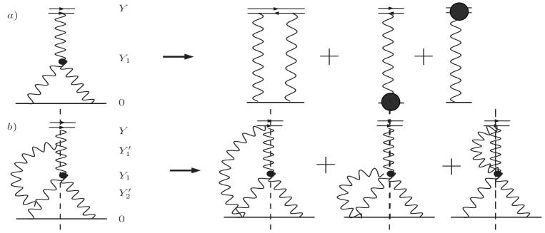
. For large mass diffraction, we have to develop a new approach. The simple form of the generating functional of Eq. (3.15) stems from the fact that the system of interacting Pomerons can be reduced to the exchange of non-interacting Pomerons after integration over rapidity $Y_{1}$, as it is shown in Fig. 2-a. In the case of diffractive production we can also calculate the Pomeron diagrams with one cut Pomeron (shown by dashed line in Fig. 2-b) but the value of $Y-Y_{1}$ is fixed, namely, $Y-Y_{1}=\ln(M^{2}/s_{0})$ where $M$ is the mass of the diffractively produced system and $s_{0}$ is the energy scale ($s_{0}\approx 1GeV^{2}$). In more complicated diagrams, we have to integrate over rapidities (for example, over $Y^{\prime}_{1}$ and $Y^{\prime}_{2}$ in Fig. 2-b). For the Pomeron with the intercept larger than 1, as in our case, these integrations result in three diagrams in Fig. 2-b. It should be stressed that the integral over the produced mass gives the dominant contribution at $Y-Y_{1}=\ln(M^{2}/s_{0})\,\approx 1/\bar{\alpha}_{S}$. However, it has not been taken into account in our eikonal - type model, which only describes the G-W contribution to the region of small mass.

Therefore, for $d\sigma/dM^{2}$ at large $M^{2}\gg s_{0}$, for one dipole $(x,y)$ we can write a generic formula (see Refs. [44])

$$M^{2}\,\frac{d\sigma^{high\;M}_{diff}}{dM^{2}}\,\,\,=\,\,\,V_{1\to 2}\left((x^{\prime},y^{\prime})\to(x^{\prime},z)+(z,y^{\prime})\right)\,\,\bigotimes\,\,\,\,\exp\left(-\Omega(s;x,y)\right)$$ (4.34)

$$\left(1-\exp\left(-\tilde{\Omega}(M^{2};x,y;x^{\prime},y^{\prime})\right)\right)\,\left[\exp\left(-\frac{1}{2}\left\{\Omega(s/M^{2};x^{\prime},z)+\Omega(s/M^{2};z,y^{\prime})\right\}\right)\,-\,\exp\left(-\frac{1}{2}\Omega(s;x^{\prime},y^{\prime})\right)\right]^{2}$$

where $\bigotimes$ denotes all needed integrations, and $\tilde{\Omega}$ is a new opacity for the interaction of two dipoles: $(x,y)$ and $(x^{\prime},y^{\prime})$, which we can build using the same approach as in Eq. (3.21). We start to analyze Eq. (4.34) considering the emission of an extra gluon (see Fig. 4).

Figure 3: The process of diffractive production in the region of large mass in perturbative QCD.

Figure 4: Feedback to the process of elastic scattering of dipole$(x,y)$ due to the emission of an extra gluon.

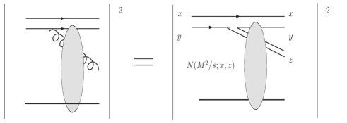
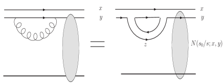
One can see that our process has three well separated stages. The first one is a penetration of the dipole $(x,y)$ through the target without inelastic interaction. We introduce the factor ”$\exp\left(-\Omega\right)$” to describe this stage. This factor sums all Pomeron diagrams with Pomerons that carry the total energy of the process( rapidity $Y$). See the second diagram in Fig. 2-b. The second stage is the emission of one extra gluon. The dipole decay is responsible for this stage with the probability given by Eq. (3.8). The last, third stage is the interaction of two produced dipoles $(x^{\prime},z)$ and $z,y^{\prime})$ with the target. This stage is taken into account in Eq. (4.34) by the factor in the brackets. This factor has been discussed in Ref. [43].

In the first diagrams (see Fig. 4) the second stage is very simple: it is just the perturbative emission of one extra gluon. The simplified formula for this diagram has the same structure as Eq. (4.34), but with a simple expression for $\exp\left(-\Omega(s;x,y)\right)\left(1-\exp\left(-\tilde{\Omega}(M^{2};x,y;x^{\prime},y^{\prime})\right)\right)$, namely

$$\sigma^{high\;M}_{diff}({Fig.~{}\ref{gem1}})\,\,=\,\,\frac{\bar{\alpha}_{S}\,n}{2}\,\,\int^{\infty}_{M^{2}_{0}}\,\frac{dM^{2}}{M^{2}}\,\,\,\int d^{2}b\int\prod^{n}_{i=1}\,dr^{2}_{i}\,\,\exp\left(-\sum^{n}_{i=2}\Omega(s/s_{0};r_{i},b)\right)\,|\Psi_{hadron}(\{r_{i}\})|^{2}\,$$

$$\left\{\exp\left(-\Omega(s/s_{0};r_{1},b)\right)\,\,r^{2}_{1}\int^{\infty}_{r^{2}_{1}}\frac{dr^{2}}{r^{4}}\,\left(1-\exp\left(-\left\{\Omega(s/M^{2};r;b)\,-\,\frac{1}{2}\Omega(s/M^{2},r_{1};b)\right\}\right)\right)^{2}\,\,\right.$$

$$\left.-\,\,r^{2}_{1}\,\int\frac{d^{2}r}{2\pi\,r^{2}\,(\vec{r}_{1}-\vec{r})^{2}}\,\left(1\,\,-\,\,\exp\left(-\Omega(s/s_{0};r_{1},b)\right)\right)^{2}\right\}$$ (4.35)

where $n$ is the number of dipoles in a proton and $\vec{r}=\vec{x}-\vec{z}$ . In Eq. (4.1) we consider the region of integration where $r_{i}\ll r$. The second term in curly brackets takes into account a change for elastic scattering of the dipole $r_{1}$ due to the emission of one extra gluon (see Fig. 4.) Eq. (4.1) is written in the leading log approximation of perturbative QCD in which we consider $\bar{\alpha}_{S}\ln(M^{2}/s_{0})\,\approx\,1$ while $\alpha_{S}\ll 1$. Factor $\left(1-\exp\left(-\Omega(s/M^{2};r)+\frac{1}{2}\Omega(s/M^{2},r_{l};b)\right)\right)$ is the amplitude of gluon-dipole scattering that has been discussed in Ref. [43]. The formulae for diffraction production is well known (see Refs. [44] for details). In the same approximation Eq. (4.34) has the form

$$M^{2}\,\frac{d\sigma^{high\;M}_{diff}}{dM^{2}}\,\,\,=\,\,\,\frac{\bar{\alpha}_{S}\,n}{2}\,\,\,\int\,d^{2}b\,\int\prod^{n}_{i=1}\,d^{2}r_{i}\,\,\,|\Psi_{hadron}(\{r_{i}\})|^{2}\,\left(\exp\left(-\Omega(s/s_{0};r_{i},b)\right)\right)\,$$ (4.36)

$$\int\,d^{2}r\,\,r^{2}\,\,\int d^{2}b^{\prime}\,\,\,\left(1-\exp\left(-\Omega^{BFKL}\left(M^{2}/s_{0};r_{i},r\right)\right)\right)\,\,\int^{\infty}_{r^{2}_{i}}\frac{dr^{\prime 2}}{r^{\prime 4}}\,\,\,\left(1-\exp\left(-\Omega(s/M^{2};r^{\prime};b)\right)\right)^{2},$$

where $\Omega^{BFKL}\left(M^{2}/s_{0};r_{i},r\right)$ is the solution of the BFKL equation with the initial condition:

$$\frac{d\,\,\Omega^{BFKL}\left(M^{2}/s_{0}=1;r_{i},r\right)}{d\ln(M^{2}/s_{0})}\,\,\,=\,\,\,\frac{\bar{\alpha}_{S}}{2}\,\delta(\vec{r}-\vec{r}^{\prime})$$ (4.37)

This $\Omega$ is equal to [5]

$$\Omega^{BFKL}\left(M^{2}/s_{0}=1;r_{i},r\right)\,\, = \,\,\int\frac{d\gamma}{2\pi\,i\,\omega(\gamma)}\,e^{\omega(\gamma)\ln(M^{2}/s_{0})\,\,+\gamma\ln(r^{2}_{i}/r^{2})}\,\,$$

$$= \,\,\sqrt{\frac{r_{i}^{2}}{r^{2}}}\,\frac{1}{\omega(0)}\,\sqrt{\frac{2\pi}{\omega"(0)\ln(M^{2}/s_{0})}}\,\,e^{\omega(0)\ln(M^{2}/s_{0})\,\,-\,\,\frac{\ln^{2}(r^{2}/r^{2}_{i})}{2\omega"(0)\,\ln(M^{2}/s_{0})}}$$

where the eigenvalues of the BFKL equation $\omega(\nu)$ can be found in Ref. [5].

The factor $1-\exp\left(-\Omega^{BFKL}\right)$ describes the inelastic cross section which in terms of the Pomeron diagrams of Fig. 2, reflects the possibility that in the fourth of Fig. 2-b, we can have two cut upper Pomerons.

We would like to stress again that Eq. (4.1) describes the dependence of the diffractive production cross section, in the region of large mass, while Eq. (4.33) is written for the low mass diffractive cross section. Therefore, to calculate the cross section for diffractive production, we need to calculate

$$\sigma_{diff}\,\,\,=\,\,\sigma^{low\;M}_{diff}\left({Eq.~{}(\ref{SDXSSM})}\right)\,\,+\,\,\sigma^{high\;M}_{diff}({Eq.~{}(\ref{SDLM})})$$ (4.39)

4.2 Hadronic wave functions

As seen from the formulae in the previous subsection, we need to know the hadronic wave functions. We have made an assumption in writing these formulae, that the correct degrees of freedom at long distances are the colorless dipoles at least at high energy[23, 24]. This is one of the strongest assumptions in our approach. It is enough to recall that for a long time the constituent quarks have been considered as a good candidate for the correct degrees of freedom in the entire range of energy. The only support for such an approach, can be seeen in the success of the Heildelberg group (see Refs. [23] and references therein), in the description of soft interactions using this ansatz.

In the case of mesons, we have only one colorless dipole and we take the transverse wave function in the form of a simple Gaussian, namely

$$|\Psi_{meson}\left(r\right)|^{2}\,\,\,=\,\,\frac{1}{\pi S^{2}_{M}}\,e^{-\frac{r^{2}}{S^{2}_{M}}}$$ (4.40)

where $S_{M}$ is a parameter that can be found from the electromagnetic radii, namely, $R_{\pi}=0.66\pm 0.01fm$ and $R_{K}=0.58\pm 0.04fm$ [40]. Using $S_{M}=\sqrt{\frac{8}{3}}R_{M}$ we obtain $S_{\pi}=1.08fm$ and $S_{K}=0.95fm$.

Figure 5: Electromagnetic (Fig. 5-a) and two gluon (Fig. 5-b) form factors. for a meson. Fig. 5-c shows the interaction of a virtual photon with a parton.

However, electromagnetic form factors gives us the space distribution of the electric charge inside of the hadron, while in our case the distribution of the density of partons (dipoles) is probed by the two gluon interaction (see Fig. 5-b). This distribution could be different from the charged one. We prefer to find the value of $S_{M}$ from the experimental data and, therefore, $S_{M}$ as well as $S_{p}$ (see below), will be the only fitting parameters in our description of the soft experimental data.

For the baryon, the situation is more complicated: we can have two or even three dipoles. Follow Ref. [23], we choose the proton wave function in the simple form for the two dipole model

$$|\Psi_{proton}(r_{1},r_{2})|^{2}\,\,=\,\,\frac{1}{(\pi\,S_{p})^{2}}\,\,e^{-\frac{r^{2}_{1}+r^{2}_{2}}{S^{2}_{p}}}$$ (4.41)

where two dipoles are defined as $\vec{r}_{1}=\vec{R}_{1}-\vec{R}_{2}$ and $\vec{r}_{2}=\vec{R}_{3}-\frac{1}{2}\left(\vec{R}_{1}+\vec{R}_{2}\right)$ where $\vec{R}_{i}$ is the position of the constituent quark $i$. In Eq. (4.41) $S_{P}=\sqrt{\frac{3}{2}}\,R_{p}\,=\,1.05fm$ for $R_{p}=0.862\pm 0.012fm$[40].

However, for large $N_{c}$ it is proven that the baryon consists of $N_{c}$ dipoles [42]. Therefore, we consider the alternative assumption for $\Psi_{proton}(r_{1},r_{2},r_{3})$, namely

$$|\Psi_{proton}(r_{1},r_{2},r_{3})|^{2}\,\,=\,\,\frac{1}{(\pi\,S_{p})^{3}}\,\,e^{-\frac{r^{2}_{1}+r^{2}_{2}\,+\,r^{2}_{3}}{S^{2}_{p}}}$$ (4.42)

where dipoles have the size $\vec{R}_{i}-\frac{1}{3}(\vec{R}_{1}+\vec{R}_{2}+\vec{R}_{3})$. In this case, from the electromagnetic radius of the proton, follows the value of $S_{p}=R_{p}=0.862\pm 0.012fm$.

In Eq. (4.41), we take the size of two dipoles to be equal. We did this for simplicity, since even in the constituent quark model (CQM), $<|r^{2}_{2}|>=4/3<|r^{2}_{1}|>$. Our hope is that the hadron interaction will be determined by the behavior of the dipole amplitude in the saturation domain, where the sensitivity to the size of dipoles is expected to be weak. On the other hand, the experimental ratio $\sigma_{tot}(\pi-p)/\sigma_{tot}(p-p)\,\approx\,2/3$ in the CQM stems from quark counting. In our approach, the dipole counting leads to the value of this ration $1/2$ (for the two dipole model for a proton) or even 1/3 (in the three dipole model) which contradicts the experimental data. The only way to obtain a reasonable description, is to hope that the perturbative QCD dependence of the dipole cross section on the size of the dipoles $\sigma\propto r^{2}$ will remain in the entire accessible range of energies. Fortunately, Ref. [24] demonstrates that this is the case, and this result encourages us to search for the description of the soft processes using the dipole hypothesis for the hadronic wave functions.

4.3 Energy variable in the model

In section 2.2 and 2.3 we have discussed our approach introducing the typical energy variable for deep inelastic scattering: $x_{Bjorken}\equiv x=Q^{2}/s$ where $Q^{2}$ is the photon virtuality and $s$ is the energy. However, with this variable we cannot discuss the soft processes which have $Q^{2}=0$. We reconsider the derivation of the Bjorken variable to introduce a new energy variable which will have a limit $x_{soft}\to x$ at $Q^{2}\gg\mu^{2}$ where $\mu$ is the scale for the soft processes. From Fig. 5-c we have a relation

$$(q+k)^{2} =-Q^{2}+x_{soft}s\,\,+\,\,k^{2}\,\,=\,\,0; x_{soft} =\left(Q^{2}+k^{2}_{\perp}\right)/s$$ (4.43)

where $q$ is the momentum of virtual photon ($q^{2}-Q^{2}$).

In Eq. (4.43) we used the fact that at high energy, $k^{2}=-k^{2}_{\perp}$. Since in the saturation domain $k^{2}_{\perp}\,\,=\,\,Q^{2}_{s}(x)$, we obtain the final expression for our energy variable

$$x_{soft} \,\,=\,\,\frac{Q^{2}+Q^{2}_{s}\left(x_{soft}\right)}{s}\,\,\xrightarrow{Q^{2}\rightarrow 0}\,\,\frac{Q^{2}_{s}\left(x_{soft}\right)}{s}; x_{soft} \,\,=\,\,\frac{Q^{2}+Q^{2}_{s}\left(x_{soft}\right)}{s}\,\,\xrightarrow{Q^{2}\gg Q^{2}_{s}}\,\,x_{Bjorken};$$ (4.44)

We believe that one of the main advantages of the saturation approach is the natural choice of the energy variable given by Eq. (4.44), which depends on the new scale: the saturation momentum.

The value of the saturation momentum in our model, we find by resolving the following equation:

$$\Omega\left(x_{soft},r^{2}_{sat}\,b=0\right)\,\,=\,\,1\,\,\,\mbox{with}\,\,r^{2}_{sat}=4/Q^{2}_{S}\left(x_{soft}\right)$$ (4.45)

Partons (dipoles) with size $r_{sat}$ are populated densely in the hadron disc, and $Q_{s}$ gives the new scale which shows that at $Q^{2}<Q^{2}_{s}$ the hard process reaches the saturation domain.

4.4 Final formulae for proton (antiproton) - proton scattering

Using the form of the proton wave function given by Eq. (4.41), we can rewrite Eq. (4.29) - Eq. (4.32) in a more accurate form, taking into account the simultaneous interaction of two dipoles (see Eq. (6)).

Figure 6: Total cross section for proton( antiproton) -proton collision taking into account the interaction of two dipoles.

For the total cross section, the general formula has the form which follows directly from Fig. 6, namely

$$\sigma_{tot}\,\,=\,\,2\,\int\,d^{2}b\,d^{2}r_{1}\,d^{2}r_{2}\,\,|\Psi_{proton}\left(r_{1},r_{2}\right)|^{2}$$ (4.46)

$$\,\,\left(N(x,r_{1};\vec{b}-\frac{1}{3}\vec{r}_{2})\,\,+\,\,N(x,r_{2};\vec{b}-\frac{1}{6}\vec{r}_{2})\,\,-\,\,N(x,r_{1};\vec{b}+\frac{1}{3}\vec{r}_{2})\,N(x,r_{2};\vec{b}+\frac{1}{6}\vec{r}_{2})\right)$$

where $\vec{b}$ is the impact parameter or the distance between $\frac{1}{3}(\vec{R}_{1}+\vec{R}_{2}+\vec{R}_{3})$ and the position of the target nucleon. One can see that we need to replace

$$\sum^{n}_{i=1}\,\,|\Psi_{hadron}(\{r_{i}\})|^{2}\,\,N(x,r_{i};b)\,\,\longrightarrow\,\,\,|\Psi_{hadron}(r_{1},r_{2})|^{2}$$ (4.47)

$$\left(N(x,r_{1};\vec{b}-\frac{1}{3}\vec{r}_{2})\,\,+\,\,N(x,r_{2};\vec{b}-\frac{1}{6}\vec{r}_{2})\,\,-\,\,N(x,r_{1};\vec{b}+\frac{1}{3}\vec{r}_{2})\,N(x,r_{2};\vec{b}+\frac{1}{6}\vec{r}_{2})\right)$$

in all of the equations of section 3.1.

Using the explicit form of the proton wave function of Eq. (4.41), we can easily rewrite the integrals in Eq. (4.29) - Eq. (4.32), in the form

$$\int\,d^{2}b\,d^{2}r_{1}\,d^{2}r_{2}\,\,|\Psi_{proton}\left(r_{1},r_{2}\right)|^{2}$$

$$\left(N(x,r_{1};\vec{b}-\frac{1}{3}\vec{r}_{2})\,\,+\,\,N(x,r_{2};\vec{b}-\frac{1}{6}\vec{r}_{2})\,\,-\,\,N(x,r_{1};\vec{b}+\frac{1}{3}\vec{r}_{2})\,N(x,r_{2};\vec{b}+\frac{1}{6}\vec{r}_{2})\right)$$

$$= \int dr^{2}_{1}\,db^{2}_{1}\,db^{2}_{2}\,\frac{1}{S_{p}^{2}}\,\exp\left(-\frac{r^{2}_{1}+4\,b^{2}_{1}+4\,b^{2}_{2}}{S^{2}_{p}}\right)\,I_{0}\left(\frac{4}{S^{2}_{p}}b_{1}\,b_{2}\right)\,\,$$

$$\times \left(N(x,r_{1};b_{1})\,\,\,+\,\,\,N(x,r_{1};b_{2})\,\,\,-\,\,N(x,r_{1};b_{1})\,\,N(x,r_{1};b_{2})\right)$$

In Eq. (4.4), we used the formula 8.431(3) of Ref. [61].

Since the typical impact parameter increases with energy, (see the next section) and the $r^{2}/3$ is small (about $1/3\,fm$ ), we can safely neglect the shift in the definition of the impact parameters in different amplitudes, replacing

$$\sum^{n}_{i=1}\,\,|\Psi_{hadron}(\{r_{i}\})|^{2}\,\,N(x,r_{i};b)\,\,\longrightarrow\,\,\,$$ (4.49)

$$|\Psi_{hadron}(r_{1},r_{2})|^{2}\,\,\left(N(x,r_{1};\vec{b})\,\,+\,\,N(x,r_{2};\vec{b})\,\,-\,\,N(x,r_{1};\vec{b})\,N(x,r_{2};\vec{b})\right)$$

$$|\Psi_{hadron}(r_{1},r_{2})|^{2}\,\,\left(1\,\,\,-\,\,\,\exp\left[-\frac{1}{2}\left(\Omega\left(x,r_{1};\vec{b}\right)+\Omega\left(x,r_{2};\vec{b}\right)\right)\right]\right)$$ (4.50)

This simplified formula works quite well in all the observables of section 3.1, except for $d\sigma_{el}/dt$ at large values of $t$. The formula of Eq. (4.50) has a simple generalization to the case of the three dipole proton model . In the three dipole model, for a proton the cross section has the form:

$$\sigma_{tot}\,\,=$$ (4.51)

$$2\,\int\,d^{2}b\,d^{2}r_{1}\,d^{2}r_{2}\,\,|\Psi_{proton}\left(r_{1},r_{2},r_{3}\right)|^{2}\,\,\left(1\,\,\,-\,\,\,\exp\left[-\frac{1}{2}\left(\Omega\left(x,r_{1};\vec{b}\right)+\Omega\left(x,r_{2};\vec{b}\right)+\Omega\left(x,r_{3};\vec{b}\right)\right)\right]\right)$$

It should be stressed that the second term in Eq. (4.46) plays a very important role at high energies, since it provides the observation that the cross section approaches a black disc limit. Indeed, only with this non-linear term in the region where the dipole amplitude tends to unity, ($N\to 1$) the factor in parenthesis ($2N-N^{2}$) also approaches 1 leading in the black disc regime.

4.5 Description of the soft cross sections

In the previous sections we have built our model and fitted all needed parameters using the DIS experimental data. In this section, we compare the model with the experimental data without any additional fitting parameters.

4.5.1 Total cross sections

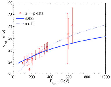
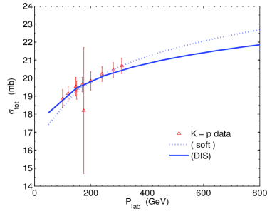
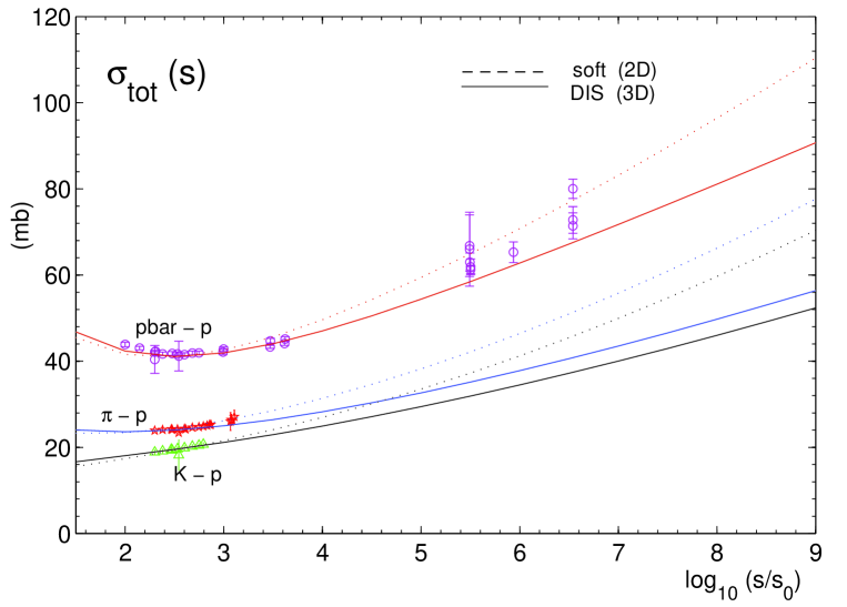
Using Eq. (4.29) , Eq. (4.40) and Eq. (4.41) we calculate the cross sections of pion-proton, kaon -proton, proton-proton and antiproton - proton scattering. The results are presented in Fig. 7 and Fig. 8. In addition to Eq. (4.29), we add a contribution of the secondary Regge trajectories using the Donnachie and Landshoff parametrization [45]. The agreement with the data is good, and shows that the saturation can replace the soft Pomeron, which has been used for fitting the soft experimental data. However, as has been mentioned, we still have one fitting parameter, namely, $S_{M}$ and $S_{p}$ in the hadron wave function. The values of $S_{\pi}$,$S_{K}$ and $S_{p}$ is given in Table 2. It is interesting to notice that the relation between the fitted values of $S$, is the same since it stems from the electromagnetic radii.

Model	$S_{\pi}$ (fm)	$S_{K}$ (fm)	$S_{p}$(fm)
A(2D)	0.515	0.552	0.561
A(3D)	0.515	0.552	0.458
B(2D)	0.556	0.597	0.615
B(3D)	0.556	0.597	0.519

Table 2: Values of parameters in hadronic wave function that give description of the soft data.

One can see that we are able to describe both the value and the energy behavior of the total cross section for meson-proton and baryon - proton interaction in our two models. However,the model B leads to a better description demonstrating, in our opinion, that the main idea to replace the phenomenological soft Pomeron by the behavior of the ’hard’ amplitude in the saturation region, is fruitful . As has been discussed in the previous subsection, the most surprising fact is that the model describes both the proton-proton and meson-proton cross sections.

Fig. 7 - a	Fig. 7 -b

Figure 7: Total cross section for $\pi-p$ (Fig. 7-a) and $K-p$ (Fig. 7-b) as a function of energy. The solid line (DIS) corresponds to the model A which describes the DIS data with $\chi^{2}/d.o.f.\,<\,1$, while the dotted line presents the model B (soft) with a worse $\chi^{2}/d.o.f.\,\approx 3$, but which leads to a better description for DIS, and soft processes data together. The number of dipoles in the proton wave function is shown in the legend.

Figure 8: Total cross section for $p\bar{p}$ scattering versus energy in our approach. Solid lines correspond to the model A, which describes the DIS data with $\chi^{2}/d.o.f.\,<\,1$, while the dotted lines present the model B (soft) with worse $\chi^{2}/d.o.f.\,\approx 3$ but which leads to a better description for DIS, and soft processes data together.

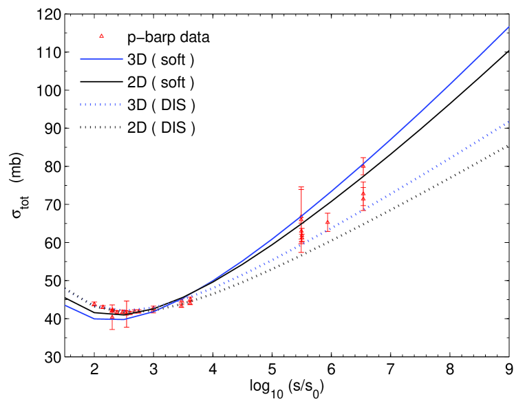
This fact can be explained only by the dependence of the dipole cross section, on the size of the dipole which the model reproduces. Since such a sensitivity can be only outside the saturation region, or close to the boundary between the saturation domain, and the perturbative QCD region. Therefore, we conclude that the soft data allow us to obtain new information on this very important transition region between the saturation and perturbative QCD region. It should be noticed that we also reproduce the difference between the interaction of pions and kaons. Since our QCD dipole cross section does not depend on the mass of the quarks, this difference also reflects the difference in the size of the dipoles, inside pion and kaon.

Figure 9: Elastic cross section for proton-proton scattering versus energy in our approach. Solid line shows the comparison with the model A with 3 dipoles in the proton wave function which described DIS with $\chi^{2}/d.o.f.\,<\,1$ while in the dotted line we plot the comparison with the experimental data the model B with $\chi^{2}/d.o.f.\,\approx\,3$ for DIS data for the two dipole model of proton.

Figure 10: Slope for the cross section for proton-proton scattering versus energy in our approach. Notations are the same as in Fig. 9.

4.5.2 Elastic cross section: energy dependence

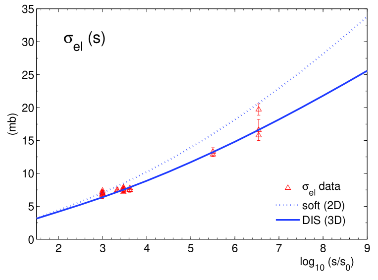
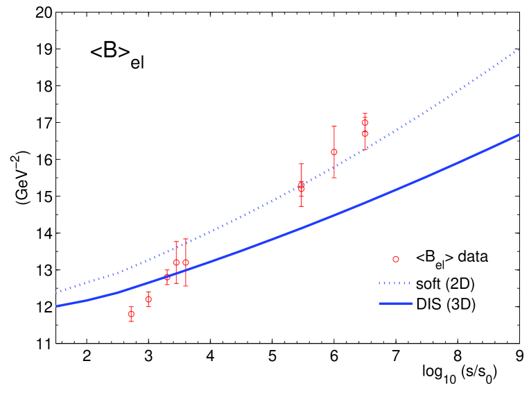
We concentrate our efforts on the proton(antiproton) interactions since meson-proton collisions have been studied experimentally only in the limited energy range (see Fig. 8). The energy dependence of the elastic cross section is presented in Fig. 9. We use Eq. (4.30) for performing our calculations. In Fig. 9 - a we compare with the experimental data our model B, while in Fig. 9 - b, is plotted our prediction for model A (three quarks). One can see that we obtain a good agreement with the experimental data, without any fitting parameter.

4.5.3 Elastic cross section: t-dependence

Using Eq. (4.32) we calculate the slope for the elastic cross section (see Fig. 10). One can see that in the model B, we reproduce the value and energy behavior of the slope at high energy, but overshoot the experimental value of this slope at sufficiently low energy. We did not include the secondary Reggeons, since we need a piece of information on the slope of the contribution of the secondary Reggeons. We also need to take into account the fact that our profile function $S(b)$ corresponds to a power-like form factor in the $t$ representation, and the value of the slope for such a function is sensitive on the range of $t$, where the slope was found experimentally. We calculate the slope at $t=0$, while the slope at an average value of $|t|=|t_{0}|>0$ is less than at $t=0$. Therefore, it is better to compare with the experimental data the $t$ dependence of the differential elastic cross section, given by Eq. (4.31). Such a comparison, one can see in Fig. 11, where the data at small $t$ is described by our model even at low energies ($\sqrt{s}=23.5GeV\,\,\mbox{and}\,\,62.5GeV$). Notice that at such low energies, the slope, that we predict, exceeds the experimental one (see Fig. 10). However, in model A, the slope is too small and, actually, this is the key difference between the two approaches. The origin for such a difference in the framework of our approach is clear: a different energy dependence of the dipole-proton amplitude in the transition region between the saturation domain, and the perturbative QCD region. Indeed, Fig. 1 shows that model B has a steeper behavior in this region in comparison with model A.

In Fig. 10 we compare our prediction with the standard phenomenological parametrization for the slope in the soft Pomeron model: $B_{el}=B_{0}+2\alpha^{\prime}\ln(s/s_{0})$ with $\alpha^{\prime}=0.25\,GeV^{-2}$ [45] and $B_{0}=9\,GeV^{-2}$. One can see that our prediction in model B is in perfect agreement with this model at high energies, while we predict a large slope at low energies. However, model A leads to a smaller slope than is seen in experiment. It should be noticed, the comparison with the experimental data (see Fig. 11) shows that model A fits the experimental data.

Figure 11: $t$-dependence of the elastic cross section for different energies at $t\,\leq\,0.6GeV^{2}$. The solid line corresponds to Model A predictions, while the dotted line describes Model B behavior of the differential cross section. Both models reproduce small $t$ behavior of the experimental data in spite of the poor description of the elastic slope in model A.

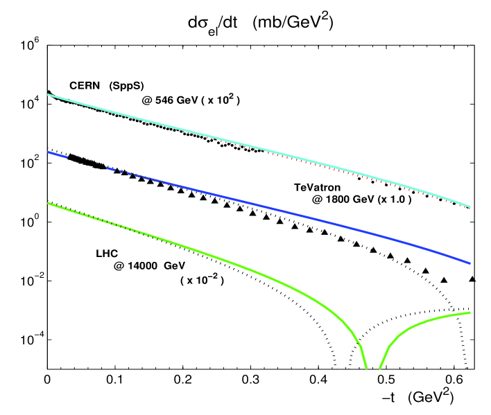
In Fig. 11 we plot the $t$-dependence for the different energy. We would like to draw your attention to two interesting features of our model B: it describes the experimental data quite well at small values of ${t}\leq 0.6\,GeV^{2}$; and it predicts the minimum at the LHC energy at rather small values of $t$ ($|t|\approx 0.45\,GeV^{2}$). The appearance of this minimum shows that our model reproduces the effective shrinkage of the diffractive peak which results in moving the typical diffractive minima in the region of smaller $t$, in comparison with lower energies. Since we did not include the real part of our scattering amplitude, we see a deep minimum. However, the real part of the amplitude will make our minima more shallow. Model A leads to a smaller value of $B_{el}$, which actually leads to a dip at large values of $t$, as compared to model B. For our rather crude models, such a description looks successful and , we hope, will encourage others to look seriously into attempts involving the description of the experimental, data based on the saturation regime of QCD.

4.5.4 Diffraction production: energy behavior of the cross section

Figure 12: Total cross section for meson-proton and proton(antiproton)-proton scattering scattering at high energies (extrapolation). Notations are the same as in Fig. 9.

In Fig. 13 the total cross section (integrated over the masses of the produced particles) of diffractive production is plotted. We use Eq. (4.34) to calculate this cross section. However, we multiply this formula by 2 since the two protons: projectile and target, can dissociate diffractively. One can see from this picture that we reproduce values and energy dependence in agreement with the experimental data. The qualitative behavior of the experimental data on $\sigma_{diff}$ versus energy is characterized by the slow dependence on energy in the region of high energies. This fact is perfectly reproduced by our model.

Figure 13: Cross section for single diffraction production for proton(antiproton)-proton scattering versus energy. The upper curves are the total cross section for diffractive production while the low curves show the energy behavior of the low mass contribution to the diffractive cross section from Eq. (4.33). Notations are the same as in Fig. 9.

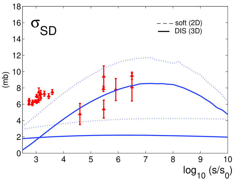
However, one can see from Fig. 13 that our approach cannot reproduce $\sigma_{SD}$ in the region of low energies (small values of produced mass). There are at least two reasons for such a failure: first, we do not take into account the exchange of the secondary Reggeons whose contribution is essential, as we see on the example of the energy behavior of the total cross section, and, second, the contribution of the one extra gluon emission has been calculated in leading log(1/x) order, which cannot describe the low mass diffraction. The experimental data on single diffraction (see Refs. [53, 52]) can be described assuming, in addition to the triple Pomeron vertex, that we modeled by extra gluon emission, a significant contribution from the Reggeon-Pomeron-Reggeon vertex in Regge phenomenology, which we cannot include in our approach.

4.6 Predictions for the LHC range of energies

As we have seen, the model is able to describe the available experimental data quite satisfactorily (and Model B even quite well) both for soft and hard interactions. Therefore, we can rely on the model B for the predictions in the LHC energy range. From Fig. 8-Fig. 13 we see that at the LHC energy we have $\sigma_{tot}=101.3\,mb$, $\sigma_{el}=28.84\,mb$ , $B_{el}=18.4\,GeV^{-2}$ and $\sigma_{diff}=10.5\,mb$ .

Model	$\sigma_{tot}$	$\sigma_{el}$	$\sigma_{diff}$	$B_{el}$	$A_{el}(b=0)$	$A_{el}(b=0)$
	mb	mb	mb	$GeV^{-2}$	(Tevatron)	(LHC)
Our A(3D)	83.0	23.54	10	16.67	0.94	0.98
Our B(2D)	101.3	28.84	10.5	18.4	0.94	0.98
GLM1[25]	110.5	25.3	11.6	20.5	0.6	0.7
GLM2[56]	91.7	20.9	11.8	17.3	0.94	0.95
RMK[55]	88.0 (86.3)	20.1 (18.1)	13.3 (16.1)	19	0.89	0.92

Table 3: Cross sections and elastic slope at the LHC energy in different models. For the RMK model, we put two parameterizations and the value for $B_{el}$ directly from the curve in Fig.18 of Ref.[55]

Table 3 shows that our prediction for LHC energy is close to ones that are given by the models that fitted the experimental data. The RMK and GLM2 models are based on soft Pomeron phenomenology while the GLM1 model is close to our approach: in this model the existence of soft Pomeron is not assumed and the parametrization was chosen for from the same ideas as our approach here. However, in the GLM1 model all parameters are found from fitting soft data. In spite the fact that the values of cross section are close the different models are different in more detailed characteristics. For example, one can see from the Table 1 they predict different values for $A_{el}(b=0)$ . From unitarity $A_{el}(b=0)\,\leq\,1$. Our model predicts that at the LHC energy our proton-proton collision is close to the black disc regime. The same we can see in GLM2 model, but in the RMK model we are not so close to this regime at the LHC, while in the GLM1 models the proton-proton interaction is far away from the black disc limit.

As you can see from Eq. (8)-c we have some information on the total cross section from the cosmic ray experiment. However, to extract the value of the total cross section from such an experiment, we need to know the meson-proton cross section as well. In Fig. 12, we plotted our predictions which we hope will be useful for discussing the cosmic ray experiment.

5 Survival probability for diffractive Higgs production

Figure 14: Diffractive Higgs production.

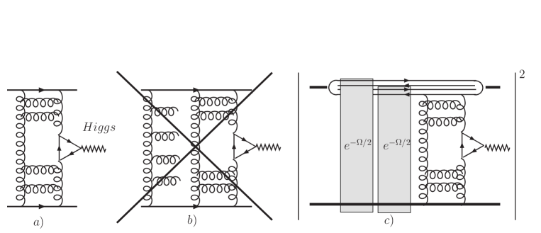
The diffractive Higgs production, is the reaction which has the best experimental signature for the discovery of the Higgs boson at the LHC. At fist sight this process occurs at short distances of the order of $1/M_{H}$, where $M_{H}$ is the mass of Higgs boson ($M_{h}\geq 100GeV$) and can be calculated in perturbative QCD (see Fig. 14-a and Ref.[46] for calculations). However, as was noticed a long ago [47, 48] that it is not enough to calculate the diagram of Fig. 14-a which describes the Higgs boson production from one parton shower. We have to multiply this cross section by a probability that two parton showers (or more) will not interact with the target since they could produced hadrons that will fill up the large rapidity gaps between Higgs and protons in the final state (see Fig. 14-b). This probability we call the survival probability. In the case of our model with the eikonal type formula for the scattering amplitude, the expression for the survival probability is very simple (see Fig. 14-c), namely,[47, 48]

$$\langle|S^{2}|\rangle\,\,\,=\,\,\frac{\int d^{2}b\,\,\left(\int d^{2}r_{1}d^{2}r_{2}|\Psi_{proton}(r_{1},r_{2})|^{2}\,e^{-\frac{1}{2}\Omega(s,r_{1},b)}\right)^{4}\,\sigma_{H}(b;{Fig.~{}\ref{spH}}-a)}{\int d^{2}b\,\sigma_{H}(b;{Fig.~{}\ref{spH}}-a)}$$ (5.52)

The appearance of the factor $\exp\left(-\frac{1}{2}\Omega(s,r_{1},b)\right)$ in Eq. (5.52) is clear from Fig. 14-c) but the power of 4 requires discussion. Actually this power reflects the fact that we have to find the probability that neither dipole 1 nor dipole 2 could scatter inelastically. The probability that one dipole does not scatter inelastically is equal to

$$\left(\int d^{2}r_{1}d^{2}r_{2}|\Psi_{proton}(r_{1},r_{2})|^{2}\,e^{-\frac{1}{2}\Omega(s,r_{1},b)}\right)^{2}\,\,\equiv\,\,\left(\langle|e^{-\frac{1}{2}\Omega(s,r_{1},b)}|\rangle\right)^{2}$$

Therefore for the probability that two dipoles cannot scatter inelastically we obtain $\left(\langle|e^{-\frac{1}{2}\Omega(s,r_{1},b)}|\rangle\right)^{4}$.

Figure 15: The value of the survival probability for diffractive Higgs production versus energy. Solid lines show the survival probability in Model A that describes the DIS data with a very good $\chi^{2}/d.o.f<1$, while dashed lines correspond to $<S^{2}>$ in Model B which gives a good description of all soft data.

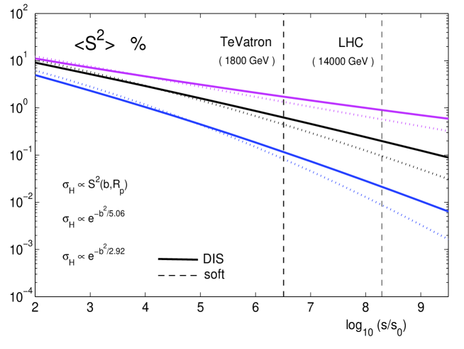
We can see from Eq. (5.52) that for the calculation of the survival probability we need to know the $b$ - dependence of the hard cross section. This dependence has been discussed in detail in Ref.[49], where it was extracted from the process of diffraction production of J$/\Psi$ with the proton (elastic) and the state with mass larger than the proton (inelastic). These two processes have two different slopes in the $t$ behavior: $B_{el}=4\,GeV^{-2}$ and $B_{in}=1.86\,GeV^{-2}$[50] . The dependence of the vertex for photon to J/$\Psi$ transition was extracted from these reactions in Ref. [51] leading to the values of slopes for the vertices of the transition of proton to proton (elastic), and proton to non-proton final state (inelastic): $B_{el}=3.6\,GeV^{-2}$ and $B_{in}=1.46\,GeV^{-2}$. In our model, the projectile proton first goes to the state of two free dipoles (see Fig. 14-c) , these two dipoles can produce two and more parton showers; and finally two free dipoles in hard processes create a proton. Therefore, at least the upper vertex is the same as in the inelastic diffractive production of J$/\Psi$ in DIS. Considering the lower vertex being elastic, we can write $\sigma_{H}(b;{Fig.~{}\ref{spH}}-a)$ in the form

$$\sigma_{H}(b;{Fig.~{}\ref{spH}}-a)\,\,\,=\,\,\,\frac{\sigma_{0}}{\pi R_{H}}\,e^{-\frac{b^{2}}{R^{2}_{H}}}$$ (5.53)

with $R^{2}_{H}=B_{in}+B_{el}=5.06\,GeV^{-2}$. However, it is our model disadvantage that we describe differently projectile and target protons. In any case the eikonal type model that we use, does not mean that only the elastic rescattering contributes to the shadowing corrections. Treating both protons on the same ground we take $R^{2}_{H}=2B_{in}=2.92\,GeV^{-2}$.

Since our model naturally includes both soft and hard interactions we can hope that the hard process of diffractive Higgs production can be described in the same way as we did in the model using the same amplitude $\Omega$. However, we need to take into account that in this case

$$\sigma_{H}(b;{Fig.~{}\ref{spH}}-a)\,\,\,=\,\,\sigma_{0}\,S^{2}(b)$$ (5.54)

where $S(b)$ is given by Eq. (3.20).

Our results on the survival probability is shown in Fig. 15, and in Table 2. Table 2 demonstrates that our value for the survival probability turns out to be much smaller than the values in the phenomenological models, that fitted the experimental data using the soft Pomeron approach (see Table 2, the review of [54] and Ref. [55]). We think that the difference stems not from the details of the models, but from the key ingredient of our model: the fact that we took into account the interaction at short distances. Therefore, we confirm that the short distances give a substantial contribution to the value of survival probability, as has been noticed in Refs. [57, 58]. The Table 2 also shows that the value of the survival probability crucially depends on the model for the $b$-dependence of the hard cross section. Our model with Eq. (5.54) for the hard cross section is similar to the one that was used in the GLM model [25]. It is interesting that our model confirms the general tendency to obtain a smaller value for the survival probability advocated in Ref. [25].

Model	$\sigma_{H}(b)$	$\langle|S^{2}|\rangle$
Our Model A(3D)	Eq. (5.53) $R^{2}_{H}=5.06\,GeV^{-2}$	0.24%
	Eq. (5.53) $R^{2}_{H}=2.92\,GeV^{-2}$	0.02%
	Eq. (5.54)	0.89%
Our Model B(2D)	Eq. (5.53) $R^{2}_{H}=5.06\,GeV^{-2}$	0.24%
	Eq. (5.53) $R^{2}_{H}=2.92\,GeV^{-2}$	0.096%
	Eq. (5.54)	0.57%
GLM1[25]	Two channel model for $\sigma_{H}$	2% (0.7%)
GLM2[56]	Two channel model for $\sigma_{H}$	0.21%
RMK[55]	Eq. (5.53) $R^{2}_{H}=11\,GeV^{-2}$	3.2% (2.3%)
	Eq. (5.53) $R^{2}_{H}\,=\,8\,GeV^{-2}$	1.7% (1.2%)

Table 4: The survival probability for diffractive Higgs production at the LHC energy, in different models. In the GLM model, for $\sigma_{H}(b)$ is used in the two channel model, with the same $B_{in}$ and $B_{el}$ for the diffractive production of J/$\Psi$ in DIS.

6 Lessons from the model

Long distance physics is very complicated, non-perturbative phenomenon, and we certainly do not pretend that we are able to describe it in its full richness. However, we demonstrate in this paper that the gap between this physics and the short distance physics which is under full control of perturbative QCD, is not so huge that it would be a hopeless task to build a bridge. Comparing this with the experimental data, we showed that the soft data depends on the transition region between saturation domain and perturbative QCD region and, therefore, can give valuable information on this transition, checking our theoretical approaches to it. The widely used, phenomenological soft Pomeron do not appear in our approach, and we hope that the reader will ask the question: do we need a soft Pomeron, having in mind our negative answer.

Our description of the experimental data, is not worse (in the case of Model B) than the one in the models which fitted the data on the basis of the soft Pomeron phenomenology (see Refs. [60, 59, 55, 25]). Recalling that we fitted all parameters of our model from DIS processes, we interpret this success in the way that the high energy soft scattering processes are determined by QCD, at short distances of the order of $1/Q_{s}$, where $Q_{s}$ is the saturation momentum. Model A describes the data worse than Model B, but we consider this description quite satisfactory remembering the crude character of this approach. It should be stressed, once more that the difference between our model A and model B, is in our attitude to the simple formula of Eq. (3.22): in model A we trust Eq. (3.22) in the entire kinematic region of accessible distances, while in model B we view this formula as a kind of qualitative description, that includes the main features of the saturation regime. Therefore, we were searching for the parameters of model B, in the way that describes all the data both on DIS, and on soft interactions, in the best possible way.

In our model, we used several assumptions which have a different theoretical status. The first assumption is the exponential form of the dipole scattering amplitude (see Eq. (3.16) and Eq. (3.22). We have discussed the theoretical arguments for such an assumption, namely, this form has been proven for the transition region between perturbative QCD, and the saturation domain (see also Ref. [12]). It should be stressed that the soft data, are sensitive to the transition region as we have discussed.

The second assumption, is the expression of Eq. (3.21) for $\Omega\left(x,r,b\right)$. This assumption is a compromise between what we should do, and what we can do. We can check it by describing the DIS experimental data, at large values of the photon virtualities, where the difference between our formula for $\Omega$, and the DGLAP expression for it should be large.

The third assumption is the impact parameter dependence of $\Omega\left(x,r,b\right)$ (see Eq. (3.19) and Eq. (3.20)). This is a pure phenomenological ansatz, since the current stage of our theory does not allow us to find $b$ dependence [28]. Actually, only soft data allows us to check this dependence. Indeed, our $\Omega$ describes the $t$-dependence of the elastic cross section while , for example, the Gaussian $b$ dependence results in the appearance of the structure of maxima and minima, at small values of $t$, which contradicts the experimental behavior of $d\sigma_{el}/dt$.

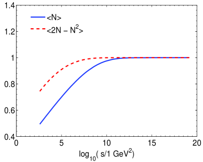
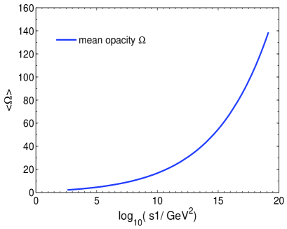
In Fig. 16-a we plot the dipole amplitude averaged with the parton wave function

$$\langle|N|\rangle|\,\,\,\equiv\,\,\,\int d^{2}r_{1}d^{2}r_{2}|\Psi_{proton}(r_{1},r_{2})|^{2}N(x,r_{1},\vec{b}=0)$$ (6.55)

One can see, that this amplitude increases and it approaches 1. However, it happens at ultra high energies and at the Tevatron energy, for example, this amplitude is only $0.8$ at $b=0$. Such an average scattering amplitude, leads to the elastic amplitude of proton-proton scattering $2N-N^{2}=0.96$. The averaged slowly increases with energy, and reaches 1 at energy. At the LHC we expect $\langle|N|\rangle=0.915$ and the average elastic amplitude is close to unity $\langle|2N-N^{2}|\rangle=0.99$. Such a behavior shows, that the values as well as the dependence on energy crucially depends on the behavior of our dipole amplitude, in the vicinity of the saturation scale. To illustrate the strength of the saturation effect, we plot the average $\Omega$ at $b=$ as a function of energy (see Fig. 16-b), which is a considerably overshoots the average scattering amplitude. It should be stressed, that in spite of the fact that the elastic amplitude is very close to unity at the LHC energy, one can see from Fig. 16-a that $\langle|N|\rangle$ is only 0.9. and the asymptotic behavior with $\langle|N|\rangle$ close to 1, starts from $s=10^{12}\,GeV^{2}$.

Fig. 16-a	Fig. 16-b

Figure 16: Average dipole amplitude ($\langle{N}\rangle$ see Eq. (6.55)), average proton- proton amplitude (both in Fig. 16-a) and average opacity $\Omega$(see Fig. 16-b) at $b=0$ as a function of energy in our model.

The principle difference between our models and the models of soft interactions, is the fact that we predict all observables fitting all parameters from the DIS data. The GLM1 model[25] is close to our approach ideologically, because it does not assume the existence of the soft Pomeron. However, at first sight this model has two major shortcomings: minima at small $t$ which have not been seen experimentally; and the slow fall down of the cross section of diffractive production, as a function of the mass of produced system of hadrons. Our model shows, that the $t$ dependence can be easily heeled by assuming the exponential form for the profile function, instead of the Gaussian one that has been used in the GLM1 model. As far as large mass diffraction that has been neglected in the GLM1 model[25], we show that this diffraction is essential. In this respect, we are close to the RMK model[55] and to the GLM2 model [56] which are based on the soft Pomeron exchange. Our model can be considered as an argument that the multi Pomeron exchanges, and the Pomeron interactions could be essential for high mass diffraction.

In general we demonstrated in this paper that the distances, essential in so called soft interactions, is not so long, but rather about $1/Q_{s}\ll R_{h}$, where $R_{h}$ is the hadron radius. This conclusion stems both from the success of our model in the description of the data, using the parameters fitted in DIS, and from the use of the energy variable $x_{soft}$, which is determined by the saturation scale.

We hope that our model will generate deeper theoretical ideas on the matching between soft and hard interactions, based on high parton density QCD.

References

- [1] L. V. Gribov, E. M. Levin and M. G. Ryskin, Phys. Rep. 100, 1 (1983).
- [2] A. H. Mueller and J. Qiu, Nucl. Phys.,427 B 268 (1986) .
- [3] L. McLerran and R. Venugopalan, Phys. Rev. D 49,2233, 3352 (1994); D 50,2225 (1994); D 53,458 (1996); D 59,09400 (1999).
-
[4]
V. N. Gribov and L. N. Lipatov, Sov. J. Nucl. Phys 15 (1972)
438;
G. Altarelli and G. Parisi,Nucl. Phys. B 126 (1977) 298;
Yu. l. Dokshitser, Sov. Phys. JETP 46 (1977) 641. - [5] E. A. Kuraev, L. N. Lipatov, and F. S. Fadin, Sov. Phys. JETP 45, 199 (1977); Ya. Ya. Balitsky and L. N. Lipatov, Sov. J. Nucl. Phys. 28, 22 (1978).
- [6] I. Balitsky, [arXiv:hep-ph/9509348]; Phys. Rev. D60, 014020 (1999) [arXiv:hep-ph/9812311] Y. V. Kovchegov, Phys. Rev. D60, 034008 (1999), [arXiv:hep-ph/9901281].
- [7] J. Jalilian-Marian, A. Kovner, A. Leonidov and H. Weigert, Phys. Rev. D59, 014014 (1999), [arXiv:hep-ph/9706377]; Nucl. Phys. B504, 415 (1997), [arXiv:hep-ph/9701284]; J. Jalilian-Marian, A. Kovner and H. Weigert, Phys. Rev. D59, 014015 (1999), [arXiv:hep-ph/9709432]; A. Kovner, J. G. Milhano and H. Weigert, Phys. Rev. D62, 114005 (2000), [arXiv:hep-ph/0004014] ; E. Iancu, A. Leonidov and L. D. McLerran, Phys. Lett. B510, 133 (2001); [arXiv:hep-ph/0102009]; Nucl. Phys. A692, 583 (2001), [arXiv:hep-ph/0011241]; E. Ferreiro, E. Iancu, A. Leonidov and L. McLerran, Nucl. Phys. A703, 489 (2002), [arXiv:hep-ph/0109115]; H. Weigert, Nucl. Phys. A703, 823 (2002), [arXiv:hep-ph/0004044].
- [8] A. Kovner and M. Lublinsky, Phys. Rev. D 71, 085004 (2005) [arXiv:hep-ph/0501198].
- [9] Y. Hatta, E. Iancu, L. McLerran, A. Stasto and D. N. Triantafyllopoulos, Nucl. Phys. A764, 423 (2006) [arXiv:hep-ph/0504182].
- [10] E. Iancu, A. H. Mueller and S. Munier, Phys. Lett. B606 (2005) 342 [arXiv:hep-ph/0410018]; E. Brunet, B. Derrida, A. H. Mueller and S. Munier, arXiv:cond-mat/0603160; Phys. Rev. E73 (2006) 056126 [arXiv:cond-mat/0512021].
- [11] R. Enberg, K. Golec-Biernat and S. Munier, Phys. Rev. D72 (2005) 074021 [arXiv:hep-ph/0505101]. S. Munier, Phys. Rev. , D 75 (2007) 034009 [arXiv:hep-ph/0608036].
- [12] E. Levin, J. Miller and A. Prygarin, “Summing Pomeron loops in the dipole approach,” Nucl.Phys. A (in press); arXiv:0706.2944 [hep-ph].
- [13] N. Armesto and M. A. Braun, Eur. Phys. J. C20, 517 (2001) [arXiv:hep-ph/0104038]; M. Lublinsky, Eur. Phys. J. C21, 513 (2001) [arXiv:hep-ph/0106112]; E. Levin and M. Lublinsky, Nucl. Phys. A712, 95 (2002) [arXiv:hep-ph/0207374]; Nucl. Phys. A712, 95 (2002) [arXiv:hep-ph/0207374]; Eur. Phys. J. C22, 647 (2002) [arXiv:hep-ph/0108239]; M. Lublinsky, E. Gotsman, E. Levin and U. Maor, Nucl. Phys. A696, 851 (2001) [arXiv:hep-ph/0102321]; Eur. Phys. J. C27, 411 (2003) [arXiv:hep-ph/0209074]; K. Golec-Biernat, L. Motyka and A.Stasto, Phys. Rev. D65, 074037 (2002) [arXiv:hep-ph/0110325]; E. Iancu, K. Itakura and S. Munier, Phys. Lett. B590 (2004) 199 [arXiv:hep-ph/0310338]. K. Rummukainen and H. Weigert, Nucl. Phys. A739, 183 (2004) [arXiv:hep-ph/0309306]; K. Golec-Biernat and A. M. Stasto, Nucl. Phys. B668, 345 (2003) [arXiv:hep-ph/0306279]; E. Gotsman, M. Kozlov, E. Levin, U. Maor and E. Naftali, Nucl. Phys. A742, 55 (2004) [arXiv:hep-ph/0401021]; K. Kutak and A. M. Stasto, Eur. Phys. J. C41, 343 (2005) [arXiv:hep-ph/0408117]; G. Chachamis, M. Lublinsky and A. Sabio Vera, Nucl. Phys. A748, 649 (2005) [arXiv:hep-ph/0408333]; J. L. Albacete, N. Armesto, J. G. Milhano, C. A. Salgado and U. A. Wiedemann, Phys. Rev. D71, 014003 (2005) [arXiv:hep-ph/0408216]; E. Gotsman, E. Levin, U. Maor and E. Naftali, Nucl. Phys. A750 (2005) 391 [arXiv:hep-ph/0411242].
- [14] K. J. Golec-Biernat and M. Wusthoff, Phys. Rev. D 59 (1999) 014017 [arXiv:hep-ph/9807513] ,̇ Phys. Rev. D 60 (1999) 114023 [arXiv:hep-ph/9903358] ; E. Gotsman, E. Levin, M. Lublinsky, U. Maor, E. Naftali and K. Tuchin, J. Phys. G 27 (2001) 2297 [arXiv:hep-ph/0010198] ; H. Kowalski and D. Teaney, Phys. Rev. D 68 (2003) 114005 [arXiv:hep-ph/0304189] ; J. Bartels, K. J. Golec-Biernat and H. Kowalski, Phys. Rev. D 66 (2002) 014001 [arXiv:hep-ph/0203258].
- [15] A. Kormilitzin, “Saturation model in the non-Glauber approach,” arXiv:0707.2202 [hep-ph].
- [16] C. Adloff et al. [H1 Collaboration], Eur. Phys. J. C 21, 33 (2001) [arXiv:hep-ex/0012053].
- [17] S. Chekanov et al. [ZEUS Collaboration], Eur. Phys. J. C 21, 443 (2001) [arXiv:hep-ex/0105090].
- [18] J. Breitweg et al. [ZEUS Collaboration], Phys. Lett. B 487, 53 (2000) [arXiv:hep-ex/0005018].
- [19] J. Bartels and E. Levin, Nucl. Phys. B387 (1992) 617.
- [20] J. Kwiecinski and A. M. Stasto, Acta Phys. Polon. B33 (2002) 3439; Phys. Rev. D66 (2002) 014013 [arXiv:hep-ph/0203030]; A. M. Stasto, K. Golec-Biernat and J. Kwiecinski, Phys. Rev. Lett. 86 (2001) 596 arXiv:hep-ph/0007192].
- [21] E. Iancu, K. Itakura and L. McLerran, Nucl. Phys. A708 (2002) 327 [arXiv:hep-ph/0203137].
- [22] L. McLerran, “Some comments about the high energy limit of QCD,” Acta Phys. Polon. B 37 (2006) 3237 [arXiv:hep-ph/0702] and references therein; E. Ferreiro, E. Iancu, K. Itakura and L. McLerran, Nucl. Phys. A 710 (2002) 373 [arXiv:hep-ph/0206241]; E. Iancu, A. Leonidov and L. McLerran, “The colour glass condensate: An introduction,” arXiv:hep-ph/0202270; E. Levin, “Saturation 2005 (mini-review),” AIP Conf. Proc. 792 (2005) 536 [arXiv:hep-ph/0506161]; “An introduction to pomerons,” arXiv:hep-ph/9808486; E. Laenen and E. Levin, “Parton Densities At High-Energy,” Ann. Rev. Nucl. Part. Sci. 44 (1994) 199; E. M. Levin and M. G. Ryskin, “High-Energy Hadron Collisions In QCD,” Phys. Rept. 189 (1990) 267.
- [23] H. G. Dosch, E. Ferreira and A. Kramer, Phys. Rev. D 50 (1994) 1992 [arXiv:hep-ph/9405237] and references therein.
- [24] J. Bartels, E. Gotsman, E. Levin, M. Lublinsky and U. Maor, Phys. Rev. D 68 (2003) 054008 [arXiv:hep-ph/0304166]; Phys. Lett. B 556 (2003) 114 [arXiv:hep-ph/0212284].
- [25] E. Gotsman, E. Levin and U. Maor, “A Soft Interaction Model at Ultra High Energies: Amplitudes, Cross Sections and Survival Probabilities,” arXiv:0708.1506 [hep-ph].
- [26] S. Munier and R. Peschanski, “Universality and tree structure of high energy QCD,” arXiv:hep-ph/0401215; Phys. Rev. D69 (2004) 034008 [arXiv:hep-ph/0310357]; Phys. Rev. Lett. 91 (2003) 232001 [arXiv:hep-ph/0309177]; A. H. Mueller and V. N. Triantafyllopoulos, Nucl.Phys. B640, 331 (2002); D. N. Triantafyllopoulos, Nucl. Phys. B 648, 293 (2003).
- [27] J. Bartels and E. Levin, Nucl. Phys. B387 (1992) 617; A. M. Stasto, K. Golec-Biernat and J. Kwiecinski, Phys. Rev. Lett., 86, 596 (2001); E. Levin and K. Tuchin, Nucl. Phys. A693 (2001) 787, [arXiv:hep-ph/0101275] ; A691 (2001) 779,[arXiv:hep-ph/0012167]; B573 (2000) 833, [arXiv:hep-ph/9908317]; E. Iancu, K. Itakura and L. McLerran, Nucl. Phys. A708, 327 (2002).
- [28] A. Kovner and U. A. Wiedemann, Phys. Lett. B 551 (2003) 311 [arXiv:hep-ph/0207335]; Phys. Rev. D 66 (2002) 034031 [arXiv:hep-ph/0204277]; Phys. Rev. D 66 (2002) 051502 [arXiv:hep-ph/0112140].
- [29] R. C. Brower, J. Polchinski, M. J. Strassler and C. I. Tan, JHEP 0712 (2007) 005 [arXiv:hep-th/0603115].
- [30] C.J. Morninstar and M. J. Peardon, Phys. Rev. D60 (2005) 344, [arXiv:hep-lat/9901004].
- [31] A. H. Mueller, Nucl. Phys. B415, 373 (1994); ibid B437, 107 (1995).
- [32] E. Levin and M. Lublinsky, Nucl. Phys. A730, 191 (2004) [arXiv:hep-ph/0308279].
- [33] E. Levin and M. Lublinsky, Phys. Lett. B607, 131 (2005) [arXiv:hep-ph/0411121].
- [34] E. Levin and K. Tuchin, Nucl. Phys. A693 (2001) 787 [arXiv:hep-ph/0101275]; A691 (2001) 779 [arXiv:hep-ph/0012167]; B573 (2000) 833 [arXiv:hep-ph/9908317].
- [35] A. H. Mueller, A. I. Shoshi and S. M. H. Wong, Nucl. Phys. B 715, 440 (2005) [arXiv:hep-ph/0501088].
- [36] E. Levin and M. Lublinsky, Nucl. Phys. A 763, 172 (2005) [arXiv:hep-ph/0501173].
- [37] E. Iancu and D. N. Triantafyllopoulos, Nucl. Phys. A756, 419 (2005) [arXiv:hep-ph/0411405]; Phys. Lett. B610, 253 (2005) [arXiv:hep-ph/0501193].
- [38] E. Gotsman, E. Levin and U. Maor, Nucl. Phys. B 464 (1996) 251 [arXiv:hep-ph/9509286] and references therein.
- [39] K. Ellis, Z. Kunst and E. Levin: Phys. Rev. D 50 (1994) 1992.
- [40] G.G. Simon et al.,Z. Naturforschung 35 A (1980) 1; S.R. Amendola et al.,Nucl. Phys. B 277 (1985) 168; Phys.Lett. B 178 (1986) 435.
- [41] M. L. Good and W. D. Walker, Phys. Rev. 120 (1960) 1857.
- [42] E. E. Jenkins, Ann. Rev. Nucl. Part. Sci. 48 (1998) 81 [arXiv:hep-ph/9803349] and references therein.
- [43] Y. V. Kovchegov and K. Tuchin, Phys. Rev. D 65 (2002) 074026 [arXiv:hep-ph/0111362].
- [44] C. Marquet, Phys. Rev. D 76 (2007) 094017 [arXiv:0706.2682 [hep-ph]]; H. Kowalski, L. Motyka and G. Watt, Phys. Rev. D 74, 074016 (2006) [arXiv:hep-ph/0606272]; Y. V. Kovchegov, Phys. Rev. D 64, 114016 (2001) [Erratum-ibid. D 68, 039901 (2003)] [arXiv:hep-ph/0107256]; Y. V. Kovchegov and L. D. McLerran, Phys. Rev. D 60, 054025 (1999) [Erratum-ibid. D 62, 019901 (2000)] [arXiv:hep-ph/9903246]; Y. V. Kovchegov, Phys. Rev. D 64, 114016 (2001) [Erratum-ibid. D 68, 039901 (2003)] [arXiv:hep-ph/0107256]; J. R. Forshaw, R. Sandapen and G. Shaw, Phys. Lett. B 594, 283 (2004) [arXiv:hep-ph/0404192]; Y. V. Kovchegov and L. D. McLerran, Phys. Rev. D 60, 054025 (1999) [Erratum-ibid. D 62, 019901 (2000)] [arXiv:hep-ph/9903246]; M. Wusthoff, Phys. Rev. D 56, 4311 (1997) [arXiv:hep-ph/9702201]; K. J. Golec-Biernat and M. Wusthoff, Phys. Rev. D 59, 014017 (1999) [arXiv:hep-ph/9807513]. E. Levin and M. Wusthoff, Phys. Rev. D 50, 4306 (1994).
- [45] A. Donnachie and P.V. Landshoff, Nucl. Phys. B231, (1984) 189; Phys. Lett. B296, (1992) 227; Zeit. Phys. C61, (1994) 139.
- [46] V. A. Khoze, A. D. Martin and M. G. Ryskin, Phys. Lett. B 650 (2007) 41 [arXiv:hep-ph/0702213]; Eur. Phys. J. C 24 (2002) 459 [arXiv:hep-ph/0201301]; Eur. Phys. J. C 26 (2002) 229 [arXiv:hep-ph/0207313] Eur. Phys. J. C 14 (2000) 525 [arXiv:hep-ph/0002072];
- [47] J. D. Bjorken, Int. J. Mod. Phys. A7, (1992) 4189; Phys. Rev. D47, (1993) 101.
- [48] E. Gotsman, E.M. Levin and U. Maor, Phys. Lett. B309, (1993) 199.
- [49] E. Gotsman, H. Kowalski, E. Levin, U. Maor and A. Prygarin, Eur. Phys. J. C47, (2006) 655.
- [50] ZEUS Collaboration, Nucl. Phys. B695 (2004) 3; Eur. Phys. J. C24 (2002) 345.
- [51] H. Kowalski and D. Teaney, Phys. Rev. D 68 (2003) 114005 [arXiv:hep-ph/0304189].
- [52] K. Goulianos and J. Montanha, Phys. Rev. D59 (1999) 114017.
- [53] F. Abe et al.(CDF Collaboration), Phys. Rev. D50 (1994) 5535.
- [54] E. Gotsman, E. Levin, U. Maor, E. Naftali and A. Prygarin, ”HERA and the LHC - A workshop on the implications of HERA for LHC physics: Proceedings Part A” (2005) 221. (arXiv:hep-ph/0511060[hep-ph]).
- [55] M. G. Ryskin, A. D. Martin and V. A. Khoze, “Soft diffraction at the LHC: a partonic interpretation,” arXiv:0710.2494 [hep-ph].
- [56] E. Gotsman, E. Levin, U. Maor and J. S. Miller, “A QCD motivated model for soft interactions at high energies,” arXiv:0805.2799 [hep-ph].
- [57] J. Bartels, S. Bondarenko, K. Kutak and L. Motyka, Phys. Rev. D73 (2006) 093004.
- [58] J. S. Miller, “Survival probability in diffractive Higgs production in high density QCD,” Eur. Phys. J. (in press) arXiv:hep-ph/0610427.
- [59] E. Gotsman, E. Levin and U. Maor, Phys. Lett. B452, (1999) 387.
- [60] E. Gotsman, E. Levin and U. Maor, Phys. Rev. D49, (1994) R4321
- [61] I. Gradstein and I. Ryzhik, “ Tables of Series, Products, and Integrals”, Verlag MIR, Moskau,1981.