The impact of priors and observables on parameter inferences in the Constrained MSSM

Abstract:

We use a newly released version of the SuperBayeS code to analyze the impact of the choice of priors and the influence of various constraints on the statistical conclusions for the preferred values of the parameters of the Constrained MSSM. We assess the effect in a Bayesian framework and compare it with an alternative likelihood-based measure of a profile likelihood. We employ a new scanning algorithm (MultiNest) which increases the computational efficiency by a factor $\sim 200$ with respect to previously used techniques. We demonstrate that the currently available data are not yet sufficiently constraining to allow one to determine the preferred values of CMSSM parameters in a way that is completely independent of the choice of priors and statistical measures. While $BR(\overline{B}\rightarrow X_{s}\gamma)$ generally favors large $m_{0}$, this is in some contrast with the preference for low values of $m_{0}$ and $m_{1/2}$ that is almost entirely a consequence of a combination of prior effects and a single constraint coming from the anomalous magnetic moment of the muon, which remains somewhat controversial. Using an information-theoretical measure, we find that the cosmological dark matter abundance determination provides at least 80% of the total constraining power of all available observables. Despite the remaining uncertainties, prospects for direct detection in the CMSSM remain excellent, with the spin-independent neutralino-proton cross section almost guaranteed above $\sigma^{SI}_{p}\sim 10^{-10}\,\mbox{pb}$, independently of the choice of priors or statistics. Likewise, gluino and lightest Higgs discovery at the LHC remain highly encouraging. While in this work we have used the CMSSM as particle physics model, our formalism and scanning technique can be readily applied to a wider class of models with several free parameters.

1 Introduction

Experiments at the Large Hadron Collider (LHC) will soon start testing many frameworks of particle physics beyond the Standard Model (SM). Particular attention will be given to the Minimal Supersymmetric SM (MSSM) and other effective low-energy models involving softly-broken supersymmetry (SUSY) which remain by far the most theoretically developed and popular schemes. On another front, dark matter (DM) experiments have by now reached the level of sensitivity that would allow them to detect a signal from DM if it is made up of the lightest neutralino, whose abundance as cold dark matter (CDM) is now very well constrained thanks to WMAP and other cosmic microwave background observations. With enough effort, Tevatron experiments may be able to improve the final LEP limit on the SM-like Higgs boson, and perhaps even detect it. Heavy quark experiments continue improving constraints on allowed contributions from “new physics” (be it SUSY or some other framework) to several observables related to flavor. Finally, an apparent discrepancy, at the level of about $3\sigma$, between experiment and SM predictions (based on $e^{+}e^{-}$ data) for the anomalous magnetic moment of the muon, has now persisted for several years.

In light of the expected vast improvement in the constraining power of data from the LHC and DM searches, it is essential to develop a solid formalism to allow one to fully explore properties of popular low-energy SUSY and other models, and to reliably derive ensuing experimental implications. Until a few years ago, a somewhat oversimplified approach based on fixed-grid scans of subsets of parameter space was sufficient. Such scans imposed observational constraints on the grid in a rigid “in-or-out” fashion (e.g., points outside some arbitrary 1 or $2\sigma$ experimental range of a given observables were discarded), without paying attention to the varying degree with which points could reproduce the data. The points on the grid surviving all the constraints were then used to qualitatively evaluate the impact of thus applied data and ensuing predictions for various observables. A major drawback of the approach was, however, that it did not allow for a probabilistic interpretation of results. A step in the right direction was to employ a chi-square analysis where, for example, the question of more properly weighting experimental errors could be addressed [1, 2, 3]. However, the approach remains of limited use as it does not allow one to perform a full scan over all relevant parameters. A major improvement in this direction has been provided by employing a Markov Chain Monte Carlo (MCMC) algorithm [4], linked with Bayesian statistics [5, 6].

Bayesian methods coupled with MCMC technology are superior in many respects to traditional, frequentist grid scans of the parameter space. (For an introduction, see, e.g., [7, 8].) For a start, they are much more efficient, in that the computational effort required to explore a parameter space of dimension $N$ scales roughly proportionally with $N$. In contrast, on a grid scan with $k$ points per dimension, the number of likelihood evaluations required goes as $k^{N}$, hence this approach becomes computationally prohibitive even for parameter space of moderate dimensionality. Secondly, the Bayesian approach allows one to easily incorporate into the final inference all relevant sources of uncertainty. For a given SUSY model one can include relevant SM (nuisance) parameters and their associated experimental errors, with the uncertainties automatically propagated to give the final uncertainty on the SUSY parameters of interest. In addition, theoretical uncertainties can be easily included in the likelihood (see [6]). Thirdly, another key advantage is the possibility to marginalize (i.e., integrate over) additional (“hidden”) dimensions in the parameter space of interest with very little computational effort. By “hidden dimensions” we mean here the parameters others than the ones being plotted, for example in 1 dimensional or 2 dimensional plots. In this paper, we upgrade our scanning technique to a much more efficient algorithm called “MultiNest” [9], which reduces very significantly the computational burden of a full exploration of the parameter space.

These advantages are built into the Bayesian procedure. The latter also requires the specification of a prior probability distribution function (or simply prior), describing our state of knowledge about the problem before we see the data. One of the main aims of this study is to assess the influence of prior choice on the statistical conclusions on CMSSM parameters. A number of recent studies have investigated the impact of several choices of priors on the parameter inference  [4, 5, 6, 10, 11, 12, 13, 14, 15, 16, 17, 18, 19] in the context of the Constrained Minimal Supersymmetric Standard Model (CMSSM) [20], and found it to be rather strong. The CMSSM, because of its relative simplicity, is a model of much interest.

The goal of the paper is twofold. On one side we address the question of the origin of the strong prior dependence. First, we point out and examine the impact on SUSY parameter inference from the highly non-linear nature of the mapping from the CMSSM parameters to the observable quantities. Next, we adopt two different priors (flat on a linear scale and flat on a log scale, see below). Within each we explore in detail, and compare, the impact of several observables which have been known to play a major role in constraining the CMSSM parameter space, including LEP bounds on Higgs properties, $BR(\overline{B}\rightarrow X_{s}\gamma)$, the relic abundance $\Omega_{\chi}h^{2}$ of the lightest neutralino assumed to constitute most of CDM in the Universe, and the anomalous magnetic moment of the muon $(g-2)_{\mu}$. It is the last observable that we find to play a singular role in favoring lower values of superparners, in some tension with some other observables, especially $BR(\overline{B}\rightarrow X_{s}\gamma)$ which favors larger scalar masses [12].

The other major aim of our paper is to compare the Bayesian posterior probability distribution with the statistical measure of a profile likelihood in the context of prior dependence. We conclude that the profile likelihood may provide a more robust assessment of the favored regions of CMSSM parameters with respect to volume effects generated by the prior choice. The coverage properties of this measure will be studied elsewhere. We focus here on the CMSSM which we treat as a case study. The problem of prior dependence is likely to be even more severe for more complicated SUSY models given present constraints, although better data such as, e.g., sparticle and Higgs detection at LHC are expected to cure it.

The paper is organized as follows. In section 2 we review the statistical formalism used in this work. In section 3 we focus on the CMSSM and introduce our experimental constraints, before exploring in section 4 the impact of priors and observables on inferences on the SUSY parameter space. In section 5 we examine in more detail the consistency of the various observational constraints and focus in particular on the tension between $(g-2)_{\mu}$ and $BR(\overline{B}\rightarrow X_{s}\gamma)$. We also quantify the information content (i.e., the constraining power) of each observable. Implications of parameter inferences on gluino and light Higgs searches at the LHC and on direct detection searches of DM are outlined in section 6, and our conclusions are presented in section 7. In Appendix A we give a brief description of the MultiNest algorithm.

2 Statistical formalism

2.1 Statistical framework

Let us denote a set of parameters of a model under consideration by $\theta$, and by $\psi$ all other relevant (so-called “nuisance parameters”). Both sets form our “basis parameters”

$$m=(\theta,\psi).$$ (1)

The cornerstone of Bayesian inference is provided by Bayes’ theorem, which reads

$$p(m|d)=\frac{p(d|\xi)\pi(m)}{p(d)}.$$ (2)

The quantity $p(m|d)$ on the l.h.s. of eq. (2) is called a posterior probability density function (posterior pdf, or simply a posterior). On the r.h.s., the quantity $p(d|\xi)$, taken as a function of $\xi$ for fixed data $d$, is called the likelihood (where the dependence $\xi(m)$ is understood). The likelihood supplies the information provided by the data. In the case of the CMSSM which we will consider below, it is constructed in Sec. 3.1 of ref. [6]. The quantity $\pi(m)$ denotes a prior probability density function (prior pdf, or simply a prior) which encodes our state of knowledge about the values of the parameters in $m$ before we see the data. The prior state of knowledge is then updated to the posterior via the likelihood. Much care must be exercised in assessing the impact of priors on the final inference on the model’s properties. If the posterior strongly depends on the choice of priors, then this is a signal that the available data is not sufficiently constraining to override the prior, and hence the information content of the posterior is strongly influenced by the choice of the prior. Therefore judgement must be suspended until more constraining data becomes available, unless there is a physically strong motivation for a specific choice of priors. (For example, in some simple situations the prior follows from considerations of the invariance properties of the problem.)

Finally, the quantity in the denominator is called evidence or model likelihood. If one is interested in constraining the model’s parameters, the evidence is merely a normalization constant, independent of $m$, and can therefore be dropped. However, the evidence is very useful in the context of Bayesian model comparison (see e.g. [21]) but in this work we will use it instead to quantify the constraining power of each observable. The evidence is a multi-dimensional integral over the model’s parameter space $m$ (including nuisance parameters),

$$p(d)=\int p(d|\xi)\pi(m){\rm d}m.$$ (3)

In our previous work [6, 11, 12, 13, 14], we employed an MCMC algorithm to map out the posterior pdf via eq. (2). As extensively described in [6], the purpose of the MCMC algorithm is to construct a sequence of points in parameter space (called “a chain”), whose density is proportional to the posterior pdf. The sequence of points thus obtained gives a series of samples from the posterior, which are weighted in such a way as to reflect the relative probability of the various regions in parameter space.

In this work we upgrade our scanning technique to use a novel algorithm, MultiNest [9], which is based on the framework of Nested Sampling, recently invented by Skilling [22]. MultiNest has been developed in such a way as to be an extremely efficient sampler even for likelihood functions defined over a parameter space of large dimensionality with a very complex structure. This aspect is very important for multi-parameter models. For example, previous MCMC scans have revealed that the 8-dimensional likelihood surface of the CMSSM can be very fragmented, and that it features many finely tuned regions that are difficult to explore with conventional MCMC and grid scans. Therefore we adopt MultiNest as an efficient sampler of the posterior. We have compared the results with our MCMC algorithm and found that they are identical (up to numerical noise). The main motivation is the increased sampling efficiency (which improves computational efficiency by a factor of $\sim 200$ with respect to our previous MCMC algorithm) and the possibility of computing automatically the Bayesian evidence, which we use in this work to quantify the amount of information in the various observables. We give a brief description of the MultiNest algorithm in Appendix A.

2.2 Statistical measures

Once a sequence of $M$ samples drawn from the posterior, $m^{(t)}$ ($t=0,1,\dots,M-1$), becomes available, it becomes a trivial task to obtain Monte Carlo estimates of expectations for any function of the parameters. For example, the posterior mean is given by

$$\langle m\rangle=\int p(m|d)m{\rm d}m\approx\frac{1}{M}\sum_{t=0}^{M-1}m^{(t)},$$ (4)

where $\langle\cdot\rangle$ denotes the expectation value with respect to the posterior and the equality with the mean of the samples follows because the samples $m^{(t)}$ are generated from the posterior by construction. In general, one can easily obtain the expectation value of any function of the parameters $f(m)$ as

$$\langle f(m)\rangle\approx\frac{1}{M}\sum_{t=0}^{M-1}f(m^{(t)}).$$ (5)

It is usually interesting to summarize the results of the inference by giving the 1–dimensional marginal probability for $m_{j}$, the $j$–th element of $m$. Taking without loss of generality $j=1$ and a parameter space of dimensionality $N$, the marginal posterior for parameter $m_{1}$ is given by

$$p(m_{1}|d)=\int p(m|d){\rm d}m_{2}\dots\rm dm_{N}.$$ (6)

From the samples it is trivial to obtain the marginal posterior on the l.h.s. of eq. (6): since the samples are drawn from the full posterior, $p(m|d)$, their density reflects the value of the full posterior pdf. It is then sufficient to divide the range of $m_{1}$ into a series of bins and count the number of samples falling within each bin, simply ignoring the coordinates values $m_{2},\dots,m_{N}$. A 2–dimensional posterior is defined in an analogous fashion. A 1D 2–tail $\alpha\%$ credible region is given by the interval (for the parameter of interest) within which fall $\alpha\%$ of the samples, obtained in such a way that a fraction $(1-\alpha)/2$ of the samples lie outside the interval on either side. In the case of a 1–tail upper (lower) limit, we report the value of the quantity below (above) which $\alpha\%$ of the sample are to be found.

An alternative statistical measure to the marginal posterior given by (6) is the profile likelihood, defined, say, for the parameter $m_{1}$ as

$${\mathfrak{L}}(m_{1})\equiv\max_{m_{2},\dots,m_{N}}\mathcal{L}(d|m),$$ (7)

where in our case $\mathcal{L}(d|m)$ is the full likelihood function. Thus in the profile likelihood one maximises the value of the likelihood along the hidden dimensions, rather than integrating it out as in the marginal posterior. The profile likelihood is obtained from the samples by maximising the value of the likelihood in each bin, and it has been recently investigated in the context of MCMC scans of the CMSSM in  [18]. The advantage is that the profile likelihood is clearly independent of the prior. However, its numerical evaluation in a high–dimensional parameter space is in general very difficult, especially when finely tuned regions are present where the likelihood is large but whose volume is very small (for a given metric). For example, a log prior on the SUSY masses will expand the volume of the low-mass parameter region and as a consequence the algorithm will explore it in much finer detail than it would be possible with a linear prior on the masses. This might find points in parameter space that are good fits to the data and that would have otherwise been missed by a scan performed using a linear prior. This will be true of any scanning algorithm: scanning in one metric (in our language, for a given prior) might in general give a different value than the numerical evaluation of the same quantity when scanning in another metric. To the extent the different numerical evaluations of the same quantity disagree, one must of course take with a grain of salt either value. As we shall demonstrate below, the choice of priors influences the numerical efficiency with which different regions of parameter space are scanned. Therefore the numerical evaluation of the profile likelihood might in general be different for different prior (i.e., metric) choices. In the following, when we refer to the profile likelihood in connection with the scanning results, we always mean “our numerical evaluation of the profile likelihood”.

The profile likelihood can be directly interpreted as a likelihood function, except of course that it does account for the effect of the hidden parameters. Therefore one can think of plots of the profile likelihood as analogous to what would be obtained by performing a more traditional fixed-grid scan in 8–dimensions, computing the chi–square at each point at then plotting the value maximised along the hidden dimensions. We report confidence intervals from the profile likelihood obtained via the usual likelihood ratio test as follows. Starting from the best-fit value in parameter space, an $\alpha$% confidence interval encloses all parameter values for which the log–likelihood increases less than $\Delta\chi^{2}(\alpha,n)$ from the best fit value. The threshold value depends on $\alpha$ and on the number $n$ of parameters one is simultaneously considering (usually $n=1$ or $n=2$), and it is obtained by solving

$$\alpha=\int_{0}^{\Delta\chi^{2}}\chi^{2}_{n}(x){\rm d}x,$$ (8)

where $\chi^{2}_{n}(x)$ is the chi–square distribution for $n$ degrees of freedom. The MultiNest algorithm we employ is much more efficient than a standard grid scan in parameter space, and it allows one to explore the full multi-dimensional parameter space at once. Therefore our scanning algorithm when coupled with the profile likelihood can be understood as an extremely efficient shortcut for the evaluation of the minimum chi–square in a multi-dimensional parameter space. However, the MultiNest technique (or indeed, any other Bayesian procedure) is not particularly optimized to look for isolated points with large likelihood in the parameter space. This means that the profile likelihood is derived from a necessarily sparse sampling of our 8-dimensional parameter space, and it might well be that regions with large likelihood that occupy a very small volume in parameter space are missed altogether. This means that an analogous problem would appear if the scan was done with a traditional grid technique, which would find multiple maxima in the likelihood if executed in 8–dimensional parameter space (grid scans to date have never been able to deal with sufficient resolution with such a high dimensional parameter space). Nevertheless, Bayesian technology and the MultiNest algorithm give several orders of magnitude improvement in the efficiency of the scan, thereby allowing for the first time to undertake a detailed analysis of the impact of the data when applied one by one or simultaneously to the whole parameter space.

As an alternative measure to the posterior, in our previous work we employed a quantity that we called the mean quality of fit (see eq. (3.1) in [12]), which is defined as the average (over the posterior) of the chi–square. Therefore the difference between the profile likelihood and the mean quality of fit is that in the mean quality of fit the chi–square is averaged over the hidden dimensions, while in the profile likelihood it is maximised. Numerical investigation shows that the two quantities are very similar in the case of the CMSSM. We have chosen to adopt in this work the profile likelihood because of its more straightforward statistical interpretation, but we point out that our previous findings showing the mean quality of fit are very similar to what one would have obtained using the profile likelihood instead.

In Bayesian statistics, the posterior pdf encodes the full information coming from the data and the prior. Ideally, the information in the data is much stronger than the information in the prior, so effectively the posterior should be dominated by the likelihood function and the prior choice ought to be irrelevant (see fig. 2 in [7] for an illustration). Furthermore, in this case it is easy to show that the Bayesian posterior, the profile likelihood and the mean quality of fit all become identical, and therefore the conclusions from the different statistical measures agree (and are uncontroversial). If the data are not strong enough, the different statistical quantities encode different pieces of information about the parameters and may in general disagree, and the prior influence might come to dominate the result. This appears to be the case with the CMSSM with currently available constraints. One of the main aims of this work is to clarify the reasons for this prior and statistical measure dependence, and to assess how much one should be worried about it.

2.3 Information content and constraining power

The Bayesian evidence returned by the MultiNest algorithm can be employed in several ways, mainly as a tool for model comparison (see, e.g. [7]). Here we employ it to quantify the amount of information (i.e., the constraining power) of the different observables. This is encoded in the Kullback–Leibler (KL) divergence between the prior and the posterior [23]. For ease of notation, let us denote the posterior pdf by $p$ and the prior by $\pi$, as before. Then the KL divergence is defined as

$$D_{\rm KL}(p,\pi)\equiv\int p(m|d)\ln\frac{p(m|d)}{\pi(m)}{\rm d}m.$$ (9)

In virtue of Bayes’ theorem the KL divergence becomes the sum of the negative log evidence and the expectation value of the log-likelihood under the posterior:

$$D_{\rm KL}(p,\pi)=-\ln p(d)+\int p(m|d)\ln\mathcal{L}(m){\rm d}m=-\ln p(d)-\langle\chi^{2}/2\rangle.$$ (10)

The first quantity on the r.h.s. is returned by the MultiNest algorithm, while computing the expectation value of the log-likelihood (i.e., the chi–square) is trivial from the samples. It is sufficient to average the chi–square over the samples.

To gain a feeling for what the KL divergence expresses, let us compute it for a 1–dimensional case, with a Gaussian prior around 0 of variance $\Sigma^{2}$ and a Gaussian likelihood centered on $m_{\rm max}$ and variance $\sigma^{2}$. We obtain after a short calculation

$$D_{\rm KL}(p,\pi)=-\frac{1}{2}-\ln\frac{\sigma}{\Sigma}+\frac{1}{2}\left[\left(\frac{\sigma}{\Sigma}\right)^{2}\left(\frac{{m_{\rm max}}^{2}}{\sigma^{2}}-1\right)\right].$$ (11)

The second term on the r.h.s. gives the reduction in parameter space volume in going from the prior to the posterior. For informative data, $\sigma/\Sigma\ll 1$, this terms is positive and grows as the logarithm of the volume ratio. On the other hand, in the same regime the third term is small unless the maximum likelihood estimate is many standard deviations away from what we expected under the prior, i.e. for $m_{\rm max}/\sigma\gg 1$. This means that the maximum likelihood value is “surprising”, in that it is far from what our prior led us to expect. Therefore we can see that the KL divergence is a summary of the amount of information, or “surprise”, contained in the data.

Other quantities can be used to assess the constraining power of the data (see e.g. [15] for a recent application), but the KL divergence has the advantage of being firmly grounded in information theory and of having a clear interpretation.

3 Implications for the Constrained MSSM

As a theoretical particle physics framework to illustrate our procedure we use the popular Constrained MSSM [20]. Some of us have examined the model in the context of Bayesian statistics before [6, 16, 11, 12]. Here we summarize its relevant features here for completeness. Below we also list, and update, where applicable, the experimental constraints on the model.

3.1 The Constrained MSSM

In the CMSSM the parameters $m_{1/2}$, $m_{0}$ and $A_{0}$, which are specified at the GUT scale $M_{\rm GUT}\simeq 2\times 10^{16}\mbox{ GeV}$, serve as boundary conditions for evolving, for a fixed value of $\tan\beta$, the MSSM Renormalization Group Equations (RGEs) down to a low energy scale $M_{\rm SUSY}\equiv\sqrt{m_{{\widetilde{t}}_{1}}m_{{\widetilde{t}}_{2}}}$ (where $m_{{\widetilde{t}}_{1},{\widetilde{t}}_{2}}$ denote the masses of the scalar partners of the top quark), chosen so as to minimize higher order loop corrections. At $M_{\rm SUSY}$ the (1-loop corrected) conditions of electroweak symmetry breaking (EWSB) are imposed and the SUSY spectrum is computed.

Our aim is to use experimental constraints on observational quantities defined in terms of CMSSM parameters to infer the most probable values of the CMSSM quantities themselves (and the associated errors). In this paper with fix the sign of $\mu$ to be positive, in order for the model to acommodate the apparent discrepancy of the anomalous magnetic moment of the muon between experiment and SM predictions. We then denote the remaining four free CMSSM parameters by the set

$$\theta=(m_{0},m_{1/2},A_{0},\tan\beta).$$ (12)

As originally demonstrated in [5, 6], the values of the relevant SM parameters can strongly influence some of the CMSSM predictions, and, in contrast to common practice, should not be simply kept fixed at their central values. We thus introduce a set $\psi$ of so-called “nuisance parameters” of the SM parameters which are relevant to our analysis,

$$\psi=(M_{t},m_{b}(m_{b})^{\overline{MS}},\alpha_{\text{em}}(M_{Z})^{\overline{MS}},\alpha_{s}(M_{Z})^{\overline{MS}}),$$ (13)

where $M_{t}$ is the pole top quark mass. The other three parameters: $m_{b}(m_{b})^{\overline{MS}}$ – the bottom quark mass evaluated at $m_{b}$, $\alpha_{\text{em}}(M_{Z})^{\overline{MS}}$ and $\alpha_{s}(M_{Z})^{\overline{MS}}$ – respectively the electromagnetic and the strong coupling constants evaluated at the $Z$ pole mass $M_{Z}$ – are all computed in the $\overline{MS}$ scheme.

The set of parameters $\theta$ and $\psi$ form an 8-dimensional set $m$ of our “basis parameters” (1). In terms of the basis parameters we compute a number of collider and cosmological observables, which we call “derived variables” and which we collectively denote by the set $\xi=(\xi_{1},\xi_{2},\ldots)$. The observables will be used to compare CMSSM predictions with a set of experimental data $d$, which is available either in the form of positive measurements or as limits, as discussed below.

3.2 Priors, observables and data

.

SM (nuisance)	Mean value	Uncertainty	Ref.
parameter	$\mu$	${\sigma}$ (exper.)
$M_{t}$	172.6 GeV	1.4 GeV	[24]
$m_{b}(m_{b})^{\overline{MS}}$	4.20 GeV	0.07 GeV	[25]
$\alpha_{s}(M_{Z})^{\overline{MS}}$	0.1176	0.002	[25]
$1/\alpha_{\text{em}}(M_{Z})^{\overline{MS}}$	127.955	0.03	[26]

Table 1: Experimental mean $\mu$ and standard deviation $\sigma$ adopted for the likelihood function for SM (nuisance) parameters, assumed to be described by a Gaussian distribution.

In order to estimate the impact of priors, we adopt two different choices of priors:

• flat priors in all the CMSSM parameters $m_{1/2}$, $m_{0}$, $A_{0}$ and $\tan\beta$;

• log priors, that are flat in $\log m_{1/2}$ and $\log m_{0}$, while for the other two CMSSM parameters we keep flat priors.

As regards the ranges, in both cases we take $50\mbox{ GeV}<m_{1/2},m_{0}<4\mbox{ TeV}$, $|A_{0}|<7\mbox{ TeV}$ and $2<\tan\beta<62$, as before [6, 11, 12]. Note that the above range of $m_{0}$ includes the hyperbolic branch/focus point (FP) region [27, 28] which will play an important role in our discussion because it currently favored by the constraint from $BR(\overline{B}\rightarrow X_{s}\gamma)$ [12].

The rationale for our choice of priors is that they are distinctively different. In particular, the log prior gives equal a priori weights to all decades for the parameter. For example, with a log prior there is the same a priori probability that $m_{0}$ be in the range $10\mbox{ GeV}<m_{0}<100\mbox{ GeV}$ as in the range $100\mbox{ GeV}<m_{0}<1\mbox{ TeV}$. In contrast, with a flat prior, the latter range of mass values has instead 10 times more a priori probability than the former. So the log prior expands the low-mass region and allows a much more refined scan in the parameter space region where finely tuned points can give a good fit to the data (see below). The reason why we apply different priors to $m_{1/2}$ and $m_{0}$ only is that both of them play a dominant role in the determination of the masses of the superpartners and Higgs bosons in the CMSSM.

Clearly a flat prior on a parameter set $m$ does not correspond to a flat prior on some non-linear function of it, ${\mathcal{F}}(m)$.The two priors are related by

$$\pi(\mathcal{F})=\pi(m){\Big{\arrowvert}}\frac{{\rm d}m}{{\rm d}\mathcal{F}}{\Big{\arrowvert}}.$$ (14)

Thus, in the case of non-linear dependence of $\mathcal{F}(m)$ the term $|{\rm d}m/{\rm d}\mathcal{F}|$ implies that an uninformative (flat) prior on $m$ may be strongly informative about (i.e., constraining) $\mathcal{F}$. (In a multi-dimensional case, the derivative term is replaced by the determinant of the Jacobian for the transformation.) It follows that a flat prior on $\log m$ (i.e., the log prior) corresponds to choosing a prior on $m$ of the form $\pi(m)\propto m^{-1}$. Therefore we expect that the choice of the log prior will give more statistical weight to lower values of $m_{1/2}$ and $m_{0}$ than in the case of flat priors.

Other choices of priors are possible, and indeed might be argued to be more theoretically motivated from the point of view of penalizing finely tuned regions of parameters space [17, 18, 19]. However, one would like the final inference to be as prior independent as possible, and the constraints to be driven by the likelihood, rather than by theoretical prejudices in the prior.

A related, although different issue is the choice of the parameters with which to define the model. One particularly well-known implementation of the CMSSM is one version of the so-called minimal supergravity model [29] where the parameters $\tan\beta$ and $m_{Z}$ are replaced by $\mu$ and $B$. This choice of parameterization has been advocated in [18, 19] as more “fundamental”. This is questionable in the case of the CMSSM which has originally been defined in ref. [20] in terms of the parameters (12) as an effective theory, without necessarily any reference to any underlying supergravity theory. More importantly, it is obvious that robust physical conclusions should not strongly depend on one choice of parameters of the model or another. If they do, this should serve as a warning bell that the derived statistical implications for observable quantities, like masses and cross sections, are not robust, in the same way as is the case with the dependence on priors. (Note that the impact of the same type of priors, e.g., flat, for different choice of parameterization, may be very different, as implied by eq. (14).)

Observable	Mean value	Uncertainties		ref.
	$\mu$	${\sigma}$ (exper.)	$\tau$ (theor.)
$M_{W}$	$80.398\mbox{ GeV}$	$25\mbox{ MeV}$	$15\mbox{ MeV}$	[30]
$\sin^{2}\theta_{\rm{eff}}{}$	$0.23153$	$16\times 10^{-5}$	$15\times 10^{-5}$	[30]
$\delta a_{\mu}^{\text{SUSY}}\times 10^{10}$	29.5	8.8	1.0	[31]
$BR(\overline{B}\rightarrow X_{s}\gamma)\times 10^{4}$	3.55	0.26	0.21	[32]
$\Delta M_{B_{s}}$	$17.77\mbox{ ps}^{-1}$	$0.12\mbox{ ps}^{-1}$	$2.4\mbox{ ps}^{-1}$	[33]
$BR(\overline{B}_{u}\to\tau\nu)\times 10^{4}$	$1.32$	$0.49$	$0.38$	[32]
$\Omega_{\chi}h^{2}$	0.1099	0.0062	$0.1\,\Omega_{\chi}h^{2}$	[34]
	Limit (95% CL)	$\tau$ (theor.)		ref.
$BR(\overline{B}_{s}\to\mu^{+}\mu^{-})$	$<5.8\times 10^{-8}$	14%		[35]
$m_{h}$	$>114.4\mbox{ GeV}$ (SM-like Higgs)	$3\mbox{ GeV}$		[36]
$\zeta_{h}^{2}$	$f(m_{h})$ (see text)	negligible		[36]
$m_{\tilde{q}}$	$>375$ GeV		5%	[25]
$m_{\tilde{g}}$	$>289$ GeV		5%	[25]
other sparticle masses	As in table 4 of ref. [6].

Table 2: Summary of the observables used in the analysis. Upper part: Observables for which a positive measurement has been made. $\delta a_{\mu}^{\text{SUSY}}=a_{\mu}^{\text{expt}}-a_{\mu}^{\text{SM}}$ denotes the discrepancy between the experimental value and the SM prediction of the anomalous magnetic moment of the muon $(g-2)_{\mu}$. As explained in the text, for each quantity we use a likelihood function with mean $\mu$ and standard deviation $s=\sqrt{\sigma^{2}+\tau^{2}}$, where $\sigma$ is the experimental uncertainty and $\tau$ represents our estimate of the theoretical uncertainty. Lower part: Observables for which only limits currently exist. The likelihood function is given in ref. [6], including in particular a smearing out of experimental errors and limits to include an appropriate theoretical uncertainty in the observables. $m_{h}$ stands for the light Higgs mass while $\zeta_{h}^{2}\equiv g^{2}(hZZ)_{\text{MSSM}}/g^{2}(hZZ)_{\text{SM}}$, where $g$ stands for the Higgs coupling to the $Z$ and $W$ gauge boson pairs.

For the SM parameters we assume flat priors over relatively wide ranges: $167.0\mbox{ GeV}\leq M_{t}\leq 178.2\mbox{ GeV}$, $3.92\mbox{ GeV}\leq m_{b}(m_{b})^{\overline{MS}}\leq 4.48\mbox{ GeV}$, $127.835\leq 1/\alpha_{\text{em}}(M_{Z})^{\overline{MS}}\leq 128.075$ and $0.1096\leq\alpha_{s}(M_{Z})^{\overline{MS}}\leq 0.1256$. This is expected to be irrelevant for the outcome of the analysis since the nuisance parameters are well-constrained by the data, as can be seen in table 1, where for each of the SM parameters we adopt a Gaussian likelihood with mean $\mu$ and experimental standard deviation $\sigma$. Note that, with respect to refs. [11, 12], we have updated the value of $M_{t}$.

The experimental values of the collider and cosmological observables that we apply (our derived variables) are listed in table 2, with updates relative to [12] where applicable. In our treatment of the radiative corrections to the electroweak observables $M_{W}$ and $\sin^{2}\theta_{\rm{eff}}$, starting from ref. [11] we include full two-loop and known higher order SM corrections as computed in ref. [37], as well as gluonic two-loop MSSM corrections obtained in [38]. We further update an experimental constraint from the anomalous magnetic moment of the muon $(g-2)_{\mu}$ for which a discrepancy (denoted by $\delta a_{\mu}^{\text{SUSY}}$) between measurement and SM predictions (based on $e^{+}e^{-}$ data) persists at the level of $3.2\sigma$ [31]. We will show that while this constraint on its own quite strongly prefers lower values of $m_{0}$ and $m_{1/2}$, this is in contradiction with the impact of most other observables. Once they are also included, this preference essentially disappears.

As regards $BR(\overline{B}\rightarrow X_{s}\gamma)$, with the central values of SM input parameters as given in table 1, for the new SM prediction we obtain the value of $(3.12\pm 0.21)\times 10^{-4}$. We compute SUSY contribution to $BR(\overline{B}\rightarrow X_{s}\gamma)$ following the procedure outlined in refs. [42, 43] which was extended in refs. [44, 45] to the case of general flavor mixing. In addition to full leading order corrections, we include large $\tan\beta$-enhanced terms arising from corrections coming from beyond the leading order and further include (subdominant) electroweak corrections.

The parametric uncertainty involved in the computation of $BR(\overline{B}_{u}\to\tau\nu)$ comes from using $|V_{ub}|=(4.34\pm 0.38)\times 10^{-3}$ [32] obtained from inclusive semileptonic B decays through the central value of $m_{b}(m_{b})^{\overline{MS}}$. For $\tau_{B}$ we use $1.643\pm 0.01\mbox{ ps}$ [32] and $f_{b}=0.216\pm 0.022\mbox{ GeV}$ [46], and obtain $BR(\overline{B}_{u}\to\tau\nu)^{\text{SM}}=1.56\pm 0.38\times 10^{-4}$. For the $\overline{B}_{s}\mbox{--}B_{s}$ oscillations we use the SM parametric uncertainty given by the global fit from the UTfit collaboration [47].

Regarding cosmological constraints, we use the determination of the relic abundance of cold DM based on the 5-year data from WMAP [34] to constrain the relic abundance $\Omega_{\chi}h^{2}$ of the lightest neutralino. In order to be conservative, we employ the constraint reported in table 1 of ref. [34] (mean value), obtained using WMAP data alone. The relic abundance (assuming the neutralino is the sole constituent of dark matter) is computed with high precision, including all resonance and coannihilation effects, through MicrOMEGAs [48], adding a 10% theoretical error in order to remain conservative. Note that our estimated theoretical uncertainty is of the same order as the uncertainty from current cosmological determinations of $\Omega_{\text{CDM}}h^{2}$.

We further include in our likelihood function an improved 95% CL limit on $BR(\overline{B}_{s}\to\mu^{+}\mu^{-})$ and a recent value of $\overline{B}_{s}\mbox{--}B_{s}$ mixing, $\Delta M_{B_{s}}$, which has recently been precisely measured at the Tevatron by the CDF Collaboration [33]. In both cases we use expressions from ref. [45] which include dominant large $\tan\beta$-enhanced beyond-LO SUSY contributions from Higgs penguin diagrams. Unfortunately, theoretical uncertainties, especially in lattice evaluations of $f_{B_{s}}$ are still substantial (as reflected in table 2 in the estimated theoretical error for $\Delta M_{B_{s}}$), which makes the impact of this precise measurement on constraining the CMSSM parameter space rather limited.

For the quantities for which positive measurements have been made (as listed in the upper part of table 2), we assume a Gaussian likelihood function with a variance given by the sum of the theoretical and experimental variances, as motivated by eq. (3.3) in ref. [6]. For the observables for which only lower or upper limits are available (as listed in the bottom part of table 2) we use a smoothed-out version of the likelihood function that accounts for the theoretical error in the computation of the observable, see eq. (3.5) and fig. 1 in ref. [6]. In particular, in applying a lower mass bound from LEP-II on the Higgs boson $h^{0}$ we take into account its dependence on its coupling to the $Z$ boson pairs $\zeta_{h}^{2}$, as described in detail in ref. [11]. When $\zeta_{h}^{2}\simeq 1$, the LEP-II lower bound of $114.4\mbox{ GeV}$ (95% CL) [36] applies. For arbitrary values of $\zeta_{h}$, we apply the LEP-II 95% CL bounds on $m_{h}$ and $m_{A}$, which we translate into the corresponding 95% CL bound in the $(m_{h},\zeta_{h}^{2})$ plane. We then add a conservative theoretical uncertainty $\tau(m_{h})=3\mbox{ GeV}$, following eq. (3.5) in ref. [6]. We will see that employing the full likelihood function in the $(m_{h},\zeta_{h}^{2})$ plane will allow us to discover some regions that evade the $114.4\mbox{ GeV}$ lower bound, and which would not have been seen in a scan that would have simply cut off all the points below the limit.

Finally, points that do not fulfil the conditions of radiative EWSB and/or give non-physical (tachyonic) solutions are discarded.

4 Effect of priors and of different observables

We now turn to the discussion of the effects of priors and experimental observables on the CMSSM parameter inference using Bayesian statistics and profile likelihood. We begin with some general remarks.

The choice of a prior pdf implies a certain measure on the parameter space defined by $m$. For example, the log prior will give less a priori weight to larger values of $m_{1/2}$ and $m_{0}$, thus reducing the preference for the FP region. What is most important is that the flat parameter space measure imposed on the basis parameter space via the choice of priors does not correspond to a flat measure over the space of the observables quantities $\xi$, since these are in general a strongly non-linear function of the chosen set of model’s parameters. Conversely, comparing observables quantities with experimental data leads to rather complicated implications for the basis parameters.

If the data are constraining enough, the effect of the likelihood dominates over that of the prior and one expects the prior dependence to be negligible in the final inference (based on the posterior pdf). Below we examine to what extent this is the case in the CMSSM. We note that the CMSSM is one of the most economical phenomenological models on the table – more complex models (with more free parameters) are qualitatively expected to compound the problem, given that, as we will show below, current constraints are not sufficiently strong to allow drawing prior-independent conclusions.

As regards experimental observables, since we will be interested in comparing the constraining power of different combinations of data, it is convenient to use shortcuts to designate them in shorthand. Those are given in table 3.

Shortcut	Observables included in data set
PHYS	Physicality constraints (no tachyons, EWSB, neutralino LSP)
NUIS	$M_{t},m_{b}(m_{b})^{\overline{MS}},\alpha_{s}(M_{Z})^{\overline{MS}},1/\alpha_{\text{em}}(M_{Z})^{\overline{MS}}$
COLL	$m_{h}$ and sparticle masses (limits)
CDM	$\Omega_{\chi}h^{2}$
BSG	$BR(\overline{B}\rightarrow X_{s}\gamma)$
GM2	$\delta a_{\mu}^{\text{SUSY}}=a_{\mu}^{\text{expt}}-a_{\mu}^{\text{SM}}$
EWO	$\sin^{2}\theta_{\rm{eff}}$, $M_{W}$
BPHYS	$\Delta M_{B_{s}},BR(\overline{B}_{s}\to\mu^{+}\mu^{-})$, $BR(\overline{B}_{u}\to\tau\nu)$
ALL	All of the above

Table 3: Shortcuts for different data combinations applied in the analysis. The actual data employed in the numerical analysis are given in tables 1 and 2.

4.1 Impact of priors

In this subsection we explore the impact of the flat and the log priors on the CMSSM parameters and on the predictions for the observable quantities. To set the stage, we perform a scan of the basis parameter space without imposing any experimental constraints at all, i.e., we take a constant likelihood function. We only discard points suffering from unphysicalities: no self-consistent solutions to the RGEs, no EWSB and tachyonic states. Furthermore, we require the neutralino to be the LSP in order to be the dark matter. Therefore the final list of samples only contains physical points in parameter space. Without the physicality constraint, we would have expected that such a scan would return a posterior identical to the prior, i.e., flat in the variables over which a flat prior has been imposed.

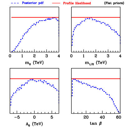
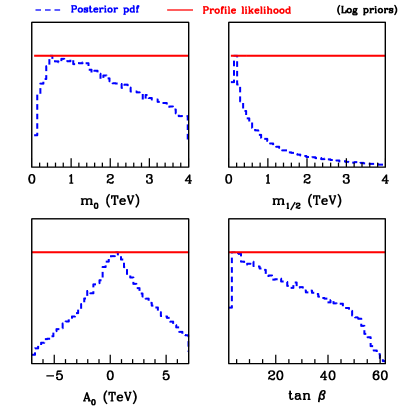
Figure 1: A scan including no experimental data, but only the requirement of physicality (PHYS). Two columns of panels on the left: 1D posterior distribution (dashed blue) and 1D profile likelihood (solid red) for the CMSSM parameters for the flat priors case. Two columns of panels on the right: the same quantities but for the log priors case. The plots reflect the prior distributions alone of the CMSSM parameters and the physicality constraints.

In fig. 1 we present the implication for 1D distributions of the posterior (dashed blue) and the profile likelihood (solid red) for the CMSSM parameters with only the physicality constraint imposed (PHYS). In the four leftmost panels we assume flat priors while in the four rightmost panels we assume log priors. (For all the SM nuisance parameters both distributions are basically flat over the prior range of the SM parameters, and we do not show them here.) Notice that the lack of samples in certain regions of parameter space, as induced by the physicality constraints, shows up in the posterior pdf as a reduction of the marginalised probability for that region. Thus for the flat priors case, the drop at low $m_{0}$ and large $m_{1/2}$ is primarily caused by the fact that in that region the LSP is the stau and hence our assumed requirements for physical points are not met. On the other hand, a gradual decrease in the posterior of $\tan\beta$ is a reflection of increasing difficulty for the RGEs to find self-consistent solutions. Eventually, at large $\tan\beta$ over about 62, the Yukawa coupling of the top quark grows to non-perturbative values before the GUT scale is reached and no solutions are found anymore, as was explained in [6]. For the log priors case, the increased a priori probability for small values of $m_{0}$ compensates the above effects, while the large $m_{0}$ region is now suppressed. The same trend is even more evident for $m_{1/2}$, where the marginal posterior pdf follows closely the expected dependence $\propto 1/m_{1/2}$ characteristic of a log prior. In contrast, the profile likelihood remains flat across all the CMSSM parameters. This is precisely what one would have expected since no data have been employed.

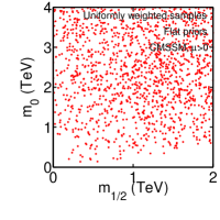
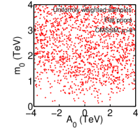
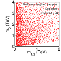
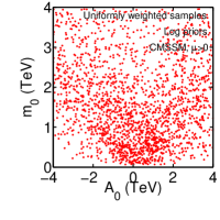
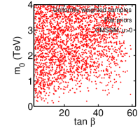
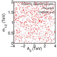
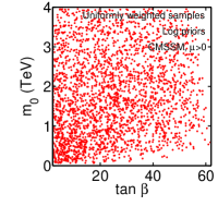
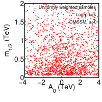
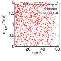
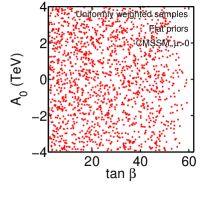
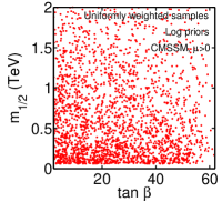
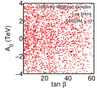
Figure 2: A scan including no experimental data, but only the requirement of physicality (PHYS), for flat priors (panels in the left two columns) and log priors (panels in the right two columns). Samples are drawn with equal weight from the prior, hence their density reflects 2D probability for different projections on the CMSSM parameters.

The above points can be confirmed by looking at the corresponding 2D distributions, which are shown in fig. 2. There we plot samples drawn with uniform weight from the prior (once the physicality constraints have been imposed), hence the density of samples reflect the prior pdf.

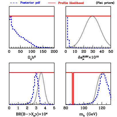
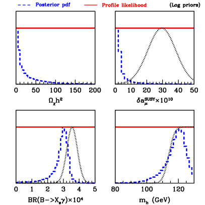
Figure 3: A scan including no experimental data, but only the requirement of physicality (PHYS). The posterior probability distribution (dashed blue) and the profile likelihood (solid red) for the most constraining observables (with flat priors on the left, and log priors on the right): the DM relic abundance $\Omega_{\chi}h^{2}$ of the neutralino, the excess in the anomalous magnetic moment of the muon $\delta a_{\mu}^{\text{SUSY}}$, the $BR(\overline{B}\rightarrow X_{s}\gamma)$ and the lightest Higgs mass $m_{h}$. For comparison, the dotted black, smooth curves give the likelihood function for the plotted observable (not imposed in this scan). For the DM abundance, the likelihood function plotted shows only the experimental error (i.e., it does not include the theoretical error employed in the scan).

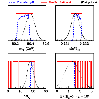
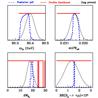
Figure 4: As in fig. 3, but for some other observables. No experimental constraints have been imposed but only the requirement of physicality (PHYS) for both flat priors (left panels) and log priors (right panels). We plot the posterior probability distribution (dashed blue) and the profile likelihood (solid red). For comparison, the dotted black, smooth curves give the likelihood function for the plotted observable (not imposed in this scan). The range of the profile likelihood (solid red line) gives the range of values for the quantities covered by the scan, as a consequence of the priors presented in section 4.

It is interesting to consider the implied distribution for the observable quantities. This can be understood as a predictive distribution from the priors and the physicality constraints for the observables. In fig. 3 we present the 1D distributions of the posterior (dashed blue) and the profile likelihood (solid red) for the quantities which will play the most important role in constraining base parameters. For comparison, for each observable we also display the likelihood function (dotted black), which however has not been imposed in this scan. The two left (right) columns are for the flat (log) prior.

Starting from the CDM abundance, we note that, in the absence of constraints from the data, for both choices of priors, the neutralino relic density is typically much larger than unity, as is well known. When we later impose the WMAP constraint (see below), we will therefore expect that the posterior will be dominated by the likelihood, since the prior is much wider (by orders of magnitude) than the likelihood. We also note that, in contrast, the profile likelihood remains flat out to much larger values — a reflection of the fact that the Bayesian posterior is suppressed because only a small number of samples is found with an extremely large relic abundance ($\Omega_{\chi}h^{2}\gg 100$).

On the other hand, the posterior for $\delta a_{\mu}^{\text{SUSY}}$ is very strongly peaked around zero. This is a consequence of the overwhelming number of samples in the FP region, where the large superpartner masses lead to a strong suppression in the SUSY contribution to $\delta a_{\mu}^{\text{SUSY}}$. Even the log prior can only give a slight extra weight to the pdf for larger values of $\delta a_{\mu}^{\text{SUSY}}$. Again, the profile likelihood is unaffected by the choice of priors.

Similar reasoning can also explain the fairly strong peak in the posterior for $BR(\overline{B}\rightarrow X_{s}\gamma)$ at $\sim 3\times 10^{-4}$, below the SM central value. This is the result of the negative (for $\mu>0$) chargino/stop contribution often overriding the always positive charged Higgs/top contribution. Finally, a large concentration of samples at large $m_{1/2}$ and $m_{0}$ also accounts for the fairly strongly peaked distribution in the pdf of the lightest Higgs mass $m_{h}$. In contrast, the profile likelihood is not affected by such volume effects, and remains flat, except for small dip at $m_{h}\sim 88\mbox{ GeV}$, well below the LEP limit (where the scan has not found any point satisfying the physicality constraints). This is likely to be the consequence of the finite number of samples we could gather.

In fig. 4 we plot the predictive distribution from the prior for the EW precision observables and $b$–physics quantities. Notice how for both choices of priors the marginal pdf implied by the prior (dashed blue) is typically much more strongly peaked than the likelihood function (dotted black). This means that the constraining power of the data for these quantities is expected to be smaller than the information already implied by the prior (see section 5.2 for more details). Therefore, as we shall explicitely show below, the impact of including them in the likelihood will be fairly limited.

To summarize, the key point is that, as we have emphasized at the beginning of this section, in the CMSSM (and, more generally, in a class of effective SUSY models where input parameters are defined at some high scale), the connection between the basis parameters and the observable quantities (other than the nuisance parameters, which obviously are directly constrained) is highly non-linear. Therefore the data, although constraining fairly strongly some of the observables, can only give indirect constraints on the parameters of the model. This is because one can move them around in order to satisfy a given constraint. Therefore plotting the posterior for the obervables in the absence of data gives the amount by which the prior measure impacts on the observable quantities. Another way of interpreting the above behavior is as the prior-predictive distribution for the observable quantities, i.e., the probability distribution for the observables implied by the choice of priors.

4.2 Impact of collider data, CDM abundance, $b\rightarrow s\gamma$ and $\delta a_{\mu}^{\text{SUSY}}$

We now move on to adding the other constraint sets from table 3 and investigate how they influence the conclusions obtained above for the two statistical measures and for our choices of priors.

First, in fig. 5 we show the CMSSM parameters (as in fig. 1) but now with data on SM nuisance parameters, collider limits on Higgs and superpartner masses and the WMAP5 CDM abundance determination added to the likelihood (PHYS+NUIS+COLL+CDM). Corresponding 2D posterior pdf and profile likelihood for some of the CMSSM variable combinations are shown in fig. 6.

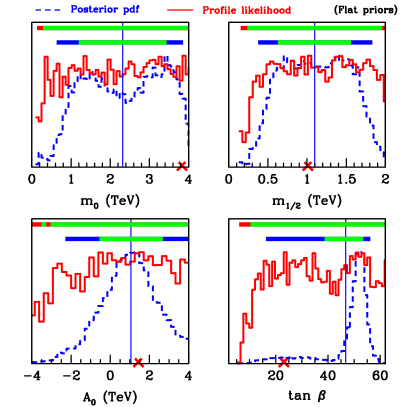
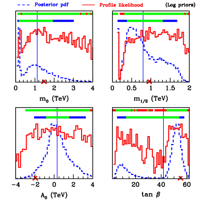
Figure 5: As in fig. 1, but now adding the constraint on SM nuisance parameters, collider limits on Higgs and superpartner masses and the WMAP5 CDM abundance determination (PHYS+NUIS+COLL+CDM), for flat/log priors (panels in the two left/right columns). The vertical, thin line is the posterior mean, the red cross the best-fit point. The horizontal bars on the top express in a graphical way the constraints on the parameters: the top bar gives 68% (green) and 95% (red) limits from the profile likelihood, while the bar below it gives 68% (green) and 95% (blue) intervals from the marginal pdf.

By examining both figures, it is clear that the resulting constraints on the CMSSM parameters depend very much on the chosen statistical measure. For example, while in the log prior case the posterior pdf shows a stronger preference smaller $m_{0}$ than with the flat prior (and a strong peak at small $m_{0}$), the profile likelihood remains essentially flat across all CMSSM parameters for both choices of priors. This is an indication that the data employed are not providing sufficient constraints on the parameters. More generally, we can see that the profile likelihood gives more conservative limits than the posterior pdf. These features can also be seen in fig. 6 (2D distributions). The 95% contours are broadly similar for both statistics for a given choice of prior, but are quite different for the two different priors. In general, the log prior favors more strongly the low energy region. We have also found that the chi-square of the best fit point (indicated by a cross) is lower for the log prior scan than the flat prior scan. There are also evident differences between the location of the best fit point and the posterior mean (indicated by a filled dot). This results from the fact the the posterior mean is influenced by the posterior distribution and its associated volume whose distribution depends fairly strongly on the chosen prior.

On the other hand, the nuisance parameters are already at this point extremely well constrained by the Gaussian likelihood, for both the Bayesian pdf and the profile likelihood statistics. The two statistics are almost identical for those variables and equal to the experimental likelihood, hence we do not show them here.

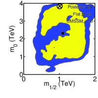
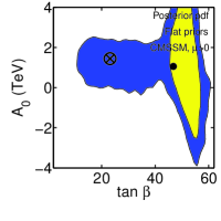
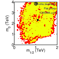
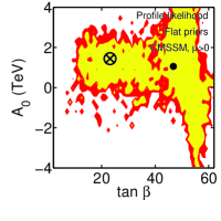
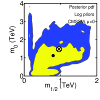
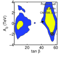
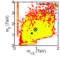
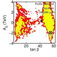
Figure 6: Posterior pdf (left two columns) and profile likelihood (right two columns) for flat priors (top row) and log priors (bottom row) for a scan including SM nuisance parameters constraints, collider limits on Higgs and superpartner masses and the WMAP5 CDM abundance determination (PHYS+NUIS+COLL+CDM). The inner and outer contours enclose respective 68% and 95% joint regions for both statistics. The posterior pdf has been smoothed with a Gaussian kernel of 1 bin width for display purposes. The cross gives the best-fit point, the filled circle is the posterior mean.

Next we add the $BR(\overline{B}\rightarrow X_{s}\gamma)$ constraint (PHYS+NUIS+COLL+CDM+BSG) in figs. 7 (1D distribution) and 8 (2D distribution). This has the effect of moving the region preferred by the profile likelihood towards large $m_{0}$ (the FP region), for both the flat and, to a lesser extent, log prior. However, the posterior pdf still suffers from a strong prior dependence, with the flat prior clearly giving more weight to larger $m_{0}$, while the log prior case strongly preferring lower $m_{0}$ and, to a lesser extent, $m_{1/2}$, a reflection of the larger a priori probability given to lower ranges of both parameters. Constraints on $\tan\beta$ are also dependent on the prior and the choice of the statistical measure.

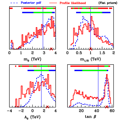
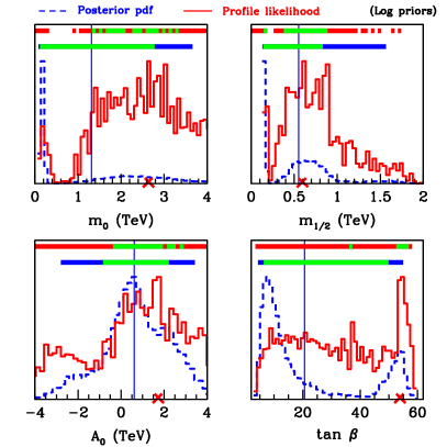
Figure 7: As in fig. 5, but with an additional constraint from $BR(\overline{B}\rightarrow X_{s}\gamma)$ (PHYS+NUIS+COLL+CDM+BSG).

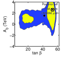
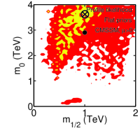
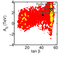
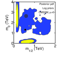
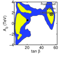
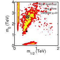
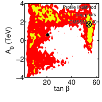
Figure 8: As in fig.  6, but with an additional constraint from $BR(\overline{B}\rightarrow X_{s}\gamma)$ (PHYS+NUIS+COLL+CDM+BSG).

In order to examine the impact of the anomalous magnetic moment of the muon, in figs. 9 (1D distribution) and 10 (2D distribution) we replace the constraint from $BR(\overline{B}\rightarrow X_{s}\gamma)$ with $\delta a_{\mu}^{\text{SUSY}}$ (PHYS+NUIS+COLL+CDM+GM2). This has the effect of moving, for both statistical measures, the prefered regions to lower masses, $m_{0},m_{1/2}\mathrel{\hbox to0.0pt{\lower 4.0pt\hbox{\hskip 1.0pt$\sim$}\hss}\raise 1.0pt\hbox{$<$}}1\mbox{ TeV}$. While there is some residual prior dependence in the posterior pdf, the profile likelihood is now almost independent of the prior and the constraints on all parameters are largely reconciled for both statistics and prior measures. This means that, in the absence of the constraint from $BR(\overline{B}\rightarrow X_{s}\gamma)$, the constraining power of the $\delta a_{\mu}^{\text{SUSY}}$ observable is rather strong.

However, such a strong constraint comes at the price of a tension with other observables which have not been included in this scan, especially $BR(\overline{B}\rightarrow X_{s}\gamma)$. This is shown in fig. 11 for the log prior (the case of the flat prior is qualitatively similar). As before, the posterior pdf is shown in dashed blue, the profile likelihood in solid red and the likelihood (data) in dotted black. The DM abundance and the $\delta a_{\mu}^{\text{SUSY}}$ are well constrained and both statistics are in agreement with the likelihood. But both the posterior and the profile likelihood for $BR(\overline{B}\rightarrow X_{s}\gamma)$ peak at a very low value, well below the SM value, reflecting a sizeable negative contribution of SUSY corrections. This is in strong diagreement with the observed likelihood. The other two $b$–physics observables exhibit a similar tension, as well. Hence we expect that, once $BR(\overline{B}\rightarrow X_{s}\gamma)$ and the other constraints are applied both the pdf and the profile likelihood will shift considerably and the $\delta a_{\mu}^{\text{SUSY}}$ constraint will produce a tension with the other data. We will discuss the tension between $\delta a_{\mu}^{\text{SUSY}}$ and the other observables in more detail in the next section.

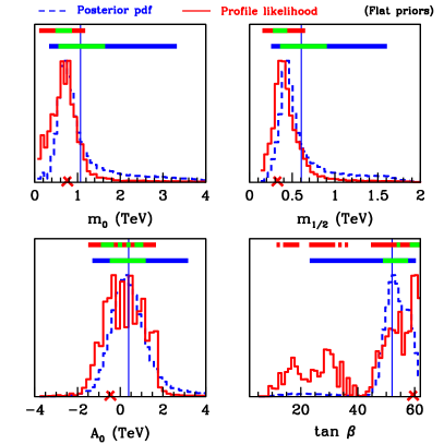
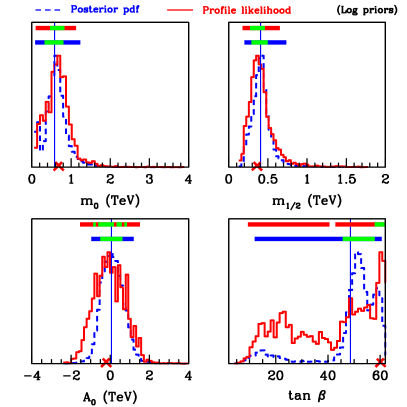
Figure 9: As in fig. 5, but with an additional constraint from $\delta a_{\mu}^{\text{SUSY}}$, instead of $BR(\overline{B}\rightarrow X_{s}\gamma)$ (PHYS+NUIS+COLL+CDM+GM2).

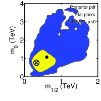
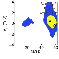
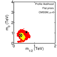
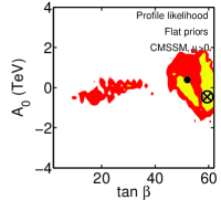
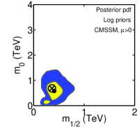
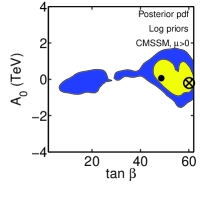
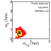
Figure 10: As in fig.  6, but with an additional constraint from $\delta a_{\mu}^{\text{SUSY}}$, instead of $BR(\overline{B}\rightarrow X_{s}\gamma)$ (PHYS+NUIS+COLL+CDM+GM2).

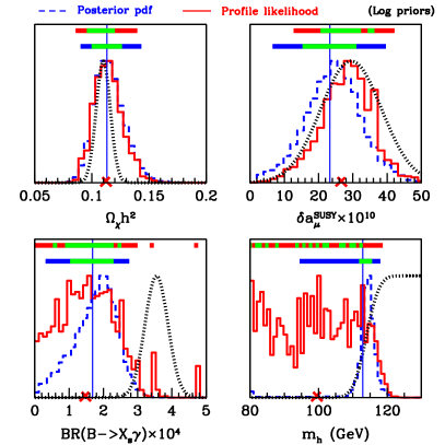
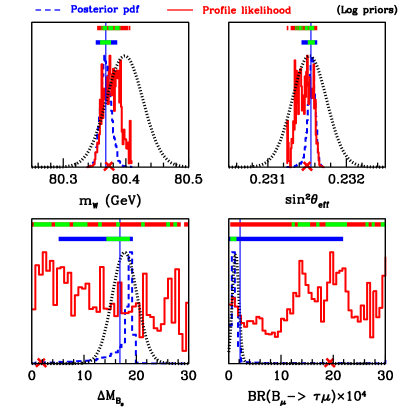
Figure 11: As in fig. 9 (PHYS+NUIS+COLL+CDM+GM2), but for several obervable quantities. Only the log priors case is shown here, the flat prior case is qualitatively similar.

4.3 Combined impact of all observables

Finally, we examine the combined effect of all the constraints listed in table 3 (ALL). The corresponding plots for the CMSSM parameters are shown in figs. 12 (1D distributions) and 13 (2D distributions). In the case of the flat prior (two leftmost columns), both posterior pdf and profile likelihood show a clear preference for large $m_{0}$ and large, but not as much, $m_{1/2}$ (the FP region), as well as a fairly narrow peak at small $m_{0}$ (the stau coannihilation region). Both statistical measures also appear to favor non-zero, positive $A_{0}$. On the other hand, the posterior shows a peak at large $\tan\beta\sim 55$, although at 95% confidence both the posterior and especially the profile likelihood allow a wide spread of values, down to small values of about 10 (where the profile likelihood shows another peak), and even less. Turning next to the log prior (two rightmost columns), the posterior for $m_{0}$ is now more strongly peaked at small values while the probability for larger values is suppressed (again as expected from a log prior). In contrast, the profile likelihood continues to indicate a preference for large $m_{0}\mathrel{\hbox to0.0pt{\lower 4.0pt\hbox{\hskip 1.0pt$\sim$}\hss}\raise 1.0pt\hbox{$>$}}1\mbox{ TeV}$, in the FP region. On the other hand, the prefered ranges of $m_{1/2}$ have for both statistical measured moved towards smaller values, as expected from the log prior, although the profile likelihood is qualitatively similar to the flat prior case. In contrast, the distributions for $A_{0}$ have not changed dramatically, while the bi-modality in the ones for $\tan\beta$ is somewhat stronger and showed more preference for lower values. We remind the reader that, for both choices of priors, we have used flat distributions in both $A_{0}$ and $\tan\beta$.

It is clear that figs. 12 and 13 are qualitatively similar to figs. 7 and 8 (which show the impact of including $BR(\overline{B}\rightarrow X_{s}\gamma)$ but not $\delta a_{\mu}^{\text{SUSY}}$), and significantly different from figs. 9 and 10 (which show impact of including $\delta a_{\mu}^{\text{SUSY}}$ but not $BR(\overline{B}\rightarrow X_{s}\gamma)$). This is yet another reflection of the strong tension between $\delta a_{\mu}^{\text{SUSY}}$ and the other constraints, mostly $BR(\overline{B}\rightarrow X_{s}\gamma)$, which at the end override to a large extent the impact of $\delta a_{\mu}^{\text{SUSY}}$.

The corresponding plots for several observables are shown in fig. 14. It is instructive to compare them with the corresponding panels in fig. 11 (where $\delta a_{\mu}^{\text{SUSY}}$ was included but not $BR(\overline{B}\rightarrow X_{s}\gamma)$) for the log prior. Again, we see a large shift in the distributions of $\delta a_{\mu}^{\text{SUSY}}$ (which now shows a strong peak in the posterior pdf near zero and a more spread-out distribution for the profile likelihood). On the other hand, the distributions for $BR(\overline{B}\rightarrow X_{s}\gamma)$ and $m_{h}$ now agree much better with the experimental data (for both statistical measures). The same remains broadly true also for the other obervables shown in fig. 14.

By examining the combined effect of all the constraints on both the CMSSM parameters on the observables themselves (figs. 12,  13 and 14), we conclude that the precise constraints are dependent on both the statistics and on the prior choice, although broad trends are apparent. This means that the combined data are not yet sufficiently strong to completely override the prior dependence. By comparing the profile likelihood for the two priors, we see that it suffers much less from prior dependence. From fig. 14 we notice that both the posterior and the profile likelihood for all of the EW and $b$-physics observables are much narrower than the likelihood, a clear sign that they are dominated by the prior distribution and that the effect of the data is solely to cut away the points preferred by $\delta a_{\mu}^{\text{SUSY}}$ (compare with fig. 11). On the other hand, the CDM abundance, $BR(\overline{B}\rightarrow X_{s}\gamma)$ and the Higgs mass limit are all in good agreement with both statistics. In contrast, the $\delta a_{\mu}^{\text{SUSY}}$ constraint cannot be easily fullfilled simultaneously, as shown by the fact that the posterior and the profile likelihood do not match with the likelihood function.

Given the tension between $\delta a_{\mu}^{\text{SUSY}}$ and the other observables we have also carried out a scan applying all observables but omitting the $\delta a_{\mu}^{\text{SUSY}}$ constraint. The results are qualitatively similar to the ones presented here, with the difference that the preference for low masses is further reduced. This further implies that indeed the $\delta a_{\mu}^{\text{SUSY}}$ constraint is to a large extent overridden by all other data preferring a different region in parameter space.

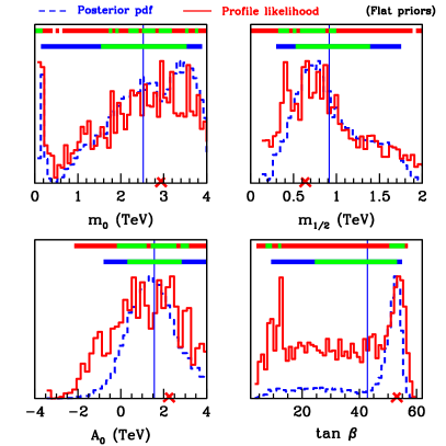
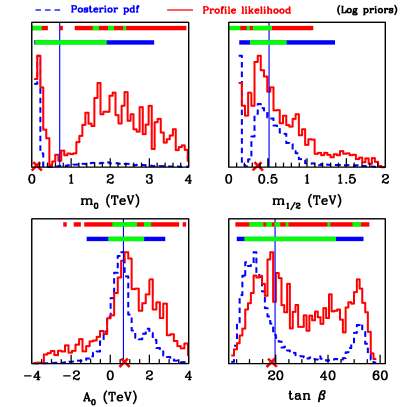
Figure 12: As in fig. 5, but for a scan including all the constraints listed in table 3 (ALL).

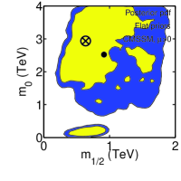
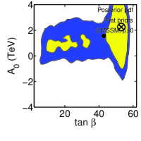
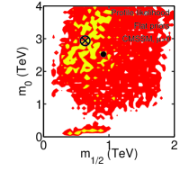
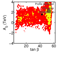
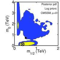
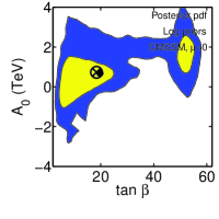
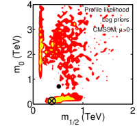
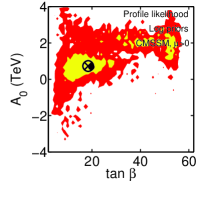
Figure 13: As in fig. 6, but but for a scan including all the constraints listed in table 3 (ALL). The change in the numerical evaluation of the profile likelihood for scans with different priors is due to the change in the efficiency with which the algorithm finds good–fitting points for the two different choices of metric, especially for small SUSY masses.

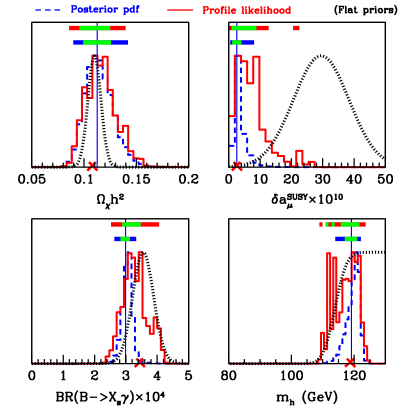
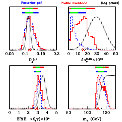
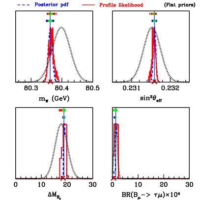
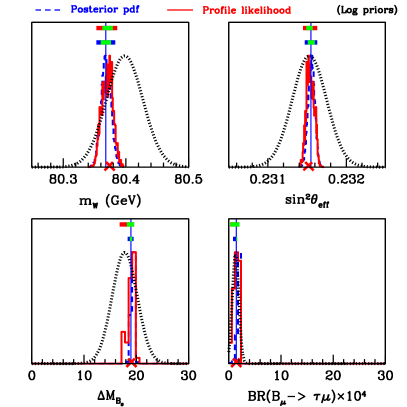
Figure 14: As in fig. 12 (ALL), but for the main observables.

5 Consistency and constraining power of the observables

We now come back to examining in more detail the tension between the constraints from $\delta a_{\mu}^{\text{SUSY}}$ and $BR(\overline{B}\rightarrow X_{s}\gamma)$ which we have already emphasized above. (Compare figs. 7 and 8 with figs. 9 and 10, respectively.)

5.1 Priors and a tension between $\delta a_{\mu}^{\text{SUSY}}$ and $BR(\overline{B}\rightarrow X_{s}\gamma)$

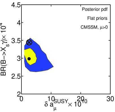
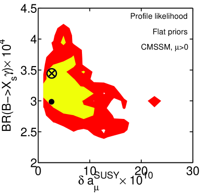
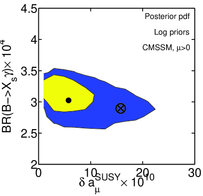
Figure 15: 2D posterior pdf (left column) and profile likelihood (right column) for $\delta a_{\mu}^{\text{SUSY}}$ and $BR(\overline{B}\rightarrow X_{s}\gamma)$ for the flat (upper row) and log priors (lower row) from a scan including constraints from all available observations (ALL). Notice that the change in the numerical evaluation of the profile likelihood for different priors is a consequence of the implicit change of metric in which the scan is executed. E.g., in the region of small SUSY masses (i.e., large $\delta a_{\mu}^{\text{SUSY}}$ values) the log prior scan is much more detailed and can find better fitting points in that region that might have been missed by the linear prior scan.

The tension is clearly exposed in fig. 15 where we include all the constraints (ALL). It is stronger with flat priors but remains substantial also in the case of log priors, and therefore stronger for the posterior pdf than for the profile likelihood since the former is more strongly prior dependent. We notice that the best fit point (cross) depends on the choice of prior quite strongly, with the log prior case able to find a point that has lower value of the masses and hence larger SUSY contributions to $\delta a_{\mu}^{\text{SUSY}}$. On the contrary, the posterior mean (circle) is very similar in both cases. This is because the posterior distribution tends to favor regions with low $\delta a_{\mu}^{\text{SUSY}}$ once all constraints are taken into account, and even the change of priors can extend the 95% contour only mildly towards larger $\delta a_{\mu}^{\text{SUSY}}$ values.

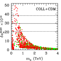
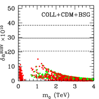
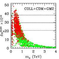
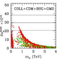
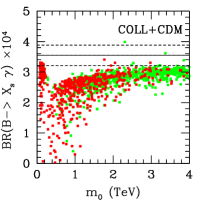
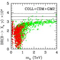
Figure 16: Distribution of samples from the posterior pdf, showing the preferred values for $\delta a_{\mu}^{\text{SUSY}}$ (top panels) and $BR(\overline{B}\rightarrow X_{s}\gamma)$ (bottom panels) for different combinations of constraints. Since the samples are drawn from the pdf, their density reflects the region’s probability. Green points are for flat priors, red for log priors. The horizontal dashed lines give the $1\sigma$ interval preferred by observations, the solid line is the central value. The samples have been thinned by a factor of 20 for visualisation purposes.

The influence of priors and their interaction with the $\delta a_{\mu}^{\text{SUSY}}$ and $BR(\overline{B}\rightarrow X_{s}\gamma)$ constraints is further investigated in fig. 16, where we plot equally weighted samples from the posterior pdf, hence the density of points represents probability density. The top panels show the probability density for $\delta a_{\mu}^{\text{SUSY}}$ vs $m_{0}$, while the bottom row shows $BR(\overline{B}\rightarrow X_{s}\gamma)$ vs $m_{0}$. Red points are for the log prior case, green for the flat prior. From left to right, we change the sets of constraints being imposed. The panels in the first column on the left have only physicality constraints, nuisance parameters constraints, Higgs and superpartner masses limits and the CDM abundance constraint imposed. The flat priors give a fairly large mass to the FP region, hence the predictions are dominated by the asymptotic SM value, $\delta a_{\mu}^{\text{SUSY}}\sim 0$ while $BR(\overline{B}\rightarrow X_{s}\gamma)\sim 3.11\times 10^{-4}$. Both observational constraints (the horizontal dashed lines give $1\sigma$ regions from the likelihood) prefer different values — hence the tension between the prior structure (and the CDM constrain) and both $\delta a_{\mu}^{\text{SUSY}}$ and $BR(\overline{B}\rightarrow X_{s}\gamma)$.

Once the $BR(\overline{B}\rightarrow X_{s}\gamma)$ constrain is further imposed (second column from the left), this has the effect of strongly shifting the preference towards the FP region, as pointed out in [12] and explained above. Notice how, as a consequence, the favored range of $\delta a_{\mu}^{\text{SUSY}}$ collapses even further towards zero, hence making the observed anomalous magnetic moment even more discrepant with the CMSSM favored range.

In contrast, imposing the $\delta a_{\mu}^{\text{SUSY}}$ constraint instead of $BR(\overline{B}\rightarrow X_{s}\gamma)$ (third column from the left) has the effect of shifting the bulk of the probability to smaller values of $m_{0}$, as low enough smuon and/or sneutrino masses are needed to produce a sufficiently large SUSY contribution to $(g-2)_{\mu}$. This, on the other hand, has the effect of selecting values of $BR(\overline{B}\rightarrow X_{s}\gamma)$ (which has not been imposed in this case) below the SM prediction, in strong disagreement with the experimental determination.

Finally, once both the $\delta a_{\mu}^{\text{SUSY}}$ and the $BR(\overline{B}\rightarrow X_{s}\gamma)$ observations are imposed (rightmost column), the posterior settles in a compromise region, which is in fair agreement with the $BR(\overline{B}\rightarrow X_{s}\gamma)$ observation but still quite discrepant with $\delta a_{\mu}^{\text{SUSY}}$. This comes about because the likelihood for $\delta a_{\mu}^{\text{SUSY}}$ is large in the region where the other constraints, and in particular $BR(\overline{B}\rightarrow X_{s}\gamma)$ (combined with the flat prior) give a very low probability.

Hence we conclude that the only observable favoring smaller values of $m_{1/2}$ and $m_{0}$ is $\delta a_{\mu}^{\text{SUSY}}$, while all the ones are either neutral or, as is the case with especially $BR(\overline{B}\rightarrow X_{s}\gamma)$, favor the FP region [12].

5.2 Quality of fit and information content

Constraints	Data	Flat priors			Log priors
	points	$\chi^{2}_{\rm min}$	$\langle\chi^{2}\rangle$	$D_{\rm KL}$	$\chi^{2}_{\rm min}$	$\langle\chi^{2}\rangle$	$D_{\rm KL}$
PHYS+NUIS	4	$0.06$	$3.89$	1.00	0.02	3.88	1.00
+CDM	5	$0.05$	$4.36$	3.22	0.10	4.32	2.59
+BSG	5	$0.31$	$6.48$	1.11	0.10	5.48	1.21
+GM2	5	$0.27$	$11.55$	1.35	0.13	6.38	1.20
+COLL+CDM	5+	$0.28$	$4.60$	3.20	0.15	5.04	2.98
+COLL+BSG	5+	$0.99$	$6.82$	1.11	0.45	6.54	1.24
+COLL+GM2	5+	$1.79$	$13.43$	1.10	0.17	9.92	1.49
+COLL+CDM+BSG	6+	$0.75$	$7.15$	3.36	0.68	7.72	3.29
+COLL+CDM+GM2	6+	$0.62$	$9.24$	2.90	0.43	7.49	3.23
+COLL+CDM+BSG+GM2	7+	$6.27$	$15.83$	3.48	4.67	14.89	3.39
ALL but GM2	10+	$3.51$	$9.45$	3.42	3.22	9.51	3.28
ALL but CDM	10+	$12.17$	$18.86$	1.10	4.14	18.30	1.24
ALL	11+	$13.51$	$19.29$	3.38	11.90	18.41	3.26

Table 4: Best-fit chi–square, $\chi^{2}_{\rm min}$, average chi-square over the posterior, $\langle\chi^{2}\rangle$, and amount of information contained in the data, quantified using the KL divergence criterion ($D_{\rm KL}$ column, given by eq. (10)). The information content has been normalized to the information from priors alone with physicality and nuisance constraints imposed (PHYS+NUIS). The column “Data points” gives the number of constraints applied, where a $+$ indicates that collider limits on the Higgs and superpartner masses have been applied.

In the light of the different constraining power of the observables, it is interesting to investigate summary statistics for the information content and the quality of fit including different combinations of data and for the two choices of priors. This is given in table 4. The information content is quantified using the KL divergence, which gives the information increase in going from the prior to the posterior, and for each prior is normalized to the information from priors alone with physicality and nuisance constraints imposed.

First, looking at the quality of fit statistics (both the minimum $\chi^{2}$ and the average of the $\chi^{2}$ over the posterior), we notice that when the $\delta a_{\mu}^{\text{SUSY}}$ constraint is added on top of $BR(\overline{B}\rightarrow X_{s}\gamma)$, the quality of fit worsens dramatically, for both choices of priors. This reflects the tension between the two observables. Even when the $\delta a_{\mu}^{\text{SUSY}}$ constraint is applied on its own (cases +GM2 and +COLL+GM2), the fit can only achieve a fairly poor average $\chi^{2}$, with the situation being worse for the linear prior scan which gives more weight to the FP region, which is at odds with the $\delta a_{\mu}^{\text{SUSY}}$ experimental value. Also, the best-fit $\chi^{2}$ is around 3 for both priors when we include all observables but $\delta a_{\mu}^{\text{SUSY}}$ (case ALL but GM2). Such a fit has nominally 2 degrees of freedom (dof), if we neglect the effect of imposing the collider limits. So a classical quality of fit test would give a $\chi^{2}/{\rm dof}$ of 1.5 which is not very large. (Although of course one has to keep in mind that such a value is difficult to interpret statistically, as clearly the $\chi^{2}$ is not chi–square distributed here!) However, when $\delta a_{\mu}^{\text{SUSY}}$ is added (case ALL), the best-fit value becomes about three times worse, giving $\chi^{2}/{\rm dof}>6$, which is clearly unacceptable. This indicate again a strong tension between $\delta a_{\mu}^{\text{SUSY}}$ and the remaining observables, which do not appear to be able to be fulfilled all at the same time within the CMSSM.

Second, the best-fit $\chi^{2}$ values and the posterior $\chi^{2}$ average are almost invariably better (albeit often not dramatically so) for the log prior scan. For the best-fit values, this is a consequence of the finer detail with which the low mass region can be explored with this prior, and therefore the scan is able to find better fitting points that can be more easily missed by the flat prior scan. The better average values reflect the fact that the log prior scan finds in general better fitting points than the flat priors one.

Finally, the information gain with respect to both priors is dominated by the CDM constraint, which alone accounts for about 80% of the combined constraining power of all the data in the log prior case and for about 95% of the constraining power for the flat prior case. This follows from taking the ratio of the $D_{\rm KL}$ value for the case +CDM with the ALL case. Taken on their own, each of the $BR(\overline{B}\rightarrow X_{s}\gamma)$ and the $\delta a_{\mu}^{\text{SUSY}}$ observables have less than half the constraining power of the CDM abundance (compare the $D_{\rm KL}$ values of the +CDM case with either +BSG or +GM2). When added on top of CDM, they only contribute about an extra 10% information on the parameters at most. This is also evident from the case ALL but CDM, where all the constraints have been applied except for the CDM abundance. In this case the information content is only very mildly increased from the PHYS+NUIS value.

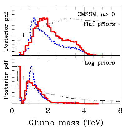
Figure 17: Posterior pdf for the gluino mass and the lightest Higgs, for flat priors (top panels) and log priors (bottom panels) for different combinations of data. The constraints applied increase with increasing line thickness. Within each panel: the dotted black line has only physicality constraints (PHYS), the blue, dashed line has physicality constraints, SM parameters constraints, collider Higgs and superpartner masses limits and CDM abundance data imposed (PHYS+NUIS+COLL+CDM), the thickest, solid red line has all constraints applied (ALL). Though not plotted in the figure, the profile likelihood show a qualitatively similar behaviour.

6 Some implications for LHC and DM searches

We now discuss some ensuing implications for prospects of experimental CMSSM tests at the LHC and in DM searches. We start by plotting in fig. 17 the posterior pdf for the gluino mass $m_{\widetilde{g}}$ and the lightest Higgs mass $m_{h}$ for the flat and log priors and for different combinations of data. (The profile likelihood has a broadly similar behavior and is not shown in the figure.) Since $m_{\widetilde{g}}\simeq 2.7m_{1/2}$, its posterior distributions (including only physicality constraints PHYS marked with dotted black; the case PHYS+NUIS+COLL+CDM with dashed blue; and all constraints, ALL, with solid red) reflect the respective plots of $m_{1/2}$ in figs. 1, 5 and 12. (Although the plot only shows the range up to $6\mbox{ TeV}$, the pdf for PHYS remains approximately flat up to $\sim 8\mbox{ TeV}$.) In the case of the flat prior one can observe a significant narrowing of the spread of $m_{\widetilde{g}}$ due to the increasing number of constraints applied (corresponding to increasing line thickness). The log prior instead (bottom left panel of fig. 17) features a shift of $m_{\widetilde{g}}$ towards lower values ($\mathrel{\hbox to0.0pt{\lower 4.0pt\hbox{\hskip 1.0pt$\sim$}\hss}\raise 1.0pt\hbox{$<$}}2\mbox{ TeV}$) almost independently of the constraining power of the data applied – a reflection of the log prior giving more weight to lower values of $m_{1/2}$ and $m_{0}$, as mentioned earlier. The dependence of $m_{\widetilde{g}}$ on the prior choice is still significant but, with the LHC reach expected to be around $2.7-3\mbox{ TeV}$, most of the gluino mass range will be explored even in the less optimistic case of the flat prior [6, 12].

Turning next to the light Higgs, in the CMSSM in most cases its couplings to $ZZ$ and $WW$ closely resemble those of the SM Higgs boson with the same mass. (However, note some exceptions mentioned in subsection 4.2.) With both priors the posterior pdf again peaks more strongly and shifts to the left with an increasing number of constraints. After all the constraints have been applied, the posterior features a rather sharp cutoff around $122\mbox{ GeV}$, similarly to the result of our detailed study [11]. (Note also that for the log prior much of the Higgs mass lies below the LEP limit on the SM-like Higgs, a reflection of our more refined treatment of the LEP limit.) This mass range is within reach of the currently operating Tevatron but will actually be rather challenging for the LHC where it may take several years to explore it.

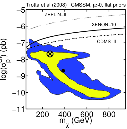
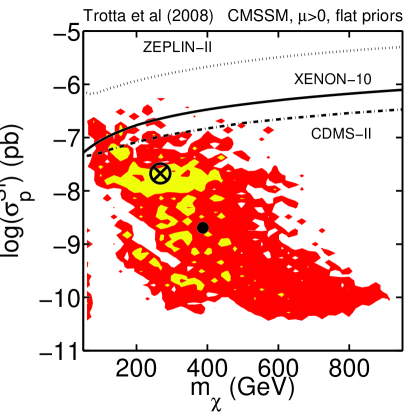
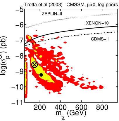
Figure 18: Posterior pdf (left column) and profile likelihood (right column) for the spin-independent scattering cross section of the neutralino WIMP off a proton versus the neutralino mass, for flat priors (top row) and log priors (bottom row), for a scan including all available constraints (ALL). The inner and outer contours enclose the respective 68% and 95% regions for both statistics. The cross gives the best-fit point, the filled circle is the posterior mean. We also plot some recent 90% upper limits for comparison (which, however, have not been included as constraints in the scan).

Finally, we investigate the implications for direct dark matter detection experiments. In fig. 18 in the plane spanned by $\sigma^{SI}_{p}$ – the spin-independent cross section for DM neutralino scattering off a proton – and the neutralino mass we plot the posterior pdf (left panels) and the profile likelihood (right panels) for the case of the flat (upper row) and log (lower row) priors. The current strongest experimental 90% CL limits from CDMS [50], XENON-10 [51] and ZEPLIN-II [52] have also been marked for comparison (athough they have not been imposed as constraints in the analysis).

Our presentation here follows our earlier studies [6, 13, 11, 12] where the direct detection quantities were discussed, accounting fully for the first time for all relevant particle physics sources of uncertainty and marginalising over nuisance parameters. (There still remain hadronic uncertainties which can change $\sigma^{SI}_{p}$ by up to a factor of ten [53].) It was shown that, with flat priors, the strong preference for the FP region leads to a rather optimistic scenario for spin-independent scattering off a nucleon, as most of the posterior probability was found to be concentrated around $\sigma^{SI}_{p}\sim 10^{-8}\,\mbox{pb}$.

Our updated results in fig. 18 still show such relatively high value (and a long $m_{\chi}$–dependent tail) for the posterior pdf for the flat prior. The profile likelihood follows a similar trend, but shows a somewhat stronger preference for large values of $\sigma^{SI}_{p}$, with the best-fit point around $\sigma^{SI}_{p}\sim 1.7\times 10^{-8}\,\mbox{pb}$. Applying the log prior (which favors lower masses) reduces significantly the contribution from the FP region. The best-fit point shifts to a value which is about one order of magnitude below the best-fit point found with the flat prior scan. (However notice from table 4 that the quality of fit of both points is very similar.) Finally, we have also investigated the case where all constraints but the $\delta a_{\mu}^{\text{SUSY}}$ observation are applied. Although this is not shown here, this case yields very similar results to the case ALL plotted in fig. 18.

The dependence on the choice of priors remains significant, which calls for caution in drawing strong conclusions regarding prospects for DM searches. Despite this, with experiments aiming to reach down to $10^{-10}\,\mbox{pb}$ most of the high-probability range of $\sigma^{SI}_{p}$ will be covered.

In conclusion, the current data are not yet constraining enough to allow one to reliably predict values of some key observables discussed here. However, even at present the predicted spread of their values make prospects for LHC searches for gluino and light Higgs (the latter also at the Tevatron) and DM searches in direct detection highly encouraging.

7 Summary and conclusions

We have subjected current constraints for the CMSSM parameters to a detailed scrutiny using a state-of-the art scanning technique (MultiNest) which reduces the computational burden by over 2 orders of magnitude with respect to previously employed MCMC techniques. We investigated the impact of prior choices and of applying different combinations of constraints, both from the point of view of Bayesian statistics and using the profile likelihood. We have updated and applied all relevant constraints, from cosmology, collider limits, EW observables, $b\rightarrow s\gamma$, $\delta a_{\mu}^{\text{SUSY}}$ and $b$–physics.

We have found that current data are not yet constraining enough to allow drawing statistically robust conclusions on allowed ranges for the CMSSM parameters. Conclusions regarding the value of $m_{0}$ and $\tan\beta$ are particularly sensitive to the choice of priors, statistics and data included. We find that in general values of $m_{1/2}\mathrel{\hbox to0.0pt{\lower 4.0pt\hbox{\hskip 1.0pt$\sim$}\hss}\raise 1.0pt\hbox{$<$}}2\mbox{ TeV}$ are preferred, while for $A_{0}$ positive values are weakly favored. We have highlighted the complex interplay between priors, observables and statistics, which intrinsically limits the constraining power of the observables on the value of the CMSSM parameters.

For this reason we feel that it is difficult to argue that one choice of parameters is in some sense or another superior to any other. In particular, the standard choice of CMSSM parameters as given by (12) is as good as the “fundamental” set in terms of $\mu$ and $B$ advocated in [18, 19]. In fact, if the choice of parameterization strongly impacts on the predictions for the measurable quantities (e.g., $\sigma^{SI}_{p}$, as in ref. [19]), this should be interpreted as a case in which theoretical prejudice plays a stronger role than the constraints from the data. Clearly, better data are required in order to be able to constrain univocally (i.e., independently of the choice of priors and statistics) the parameters of the model. This conclusion is expected to apply more generally to more complex phenomenological models, with a larger number of free parameters than the CMSSM.

Among the observables, the most constraining role is played by $\Omega_{\chi}h^{2}$, $m_{h}$, $BR(\overline{B}\rightarrow X_{s}\gamma)$ and $\delta a_{\mu}^{\text{SUSY}}$. The latter (still somewhat controversial) constraint is singular in favoring smaller $m_{1/2}$ and $m_{0}$ but in a numerical analysis its impact becomes outweighted by the other constraints, especially $BR(\overline{B}\rightarrow X_{s}\gamma)$ which favors the FP region. The numerical measure of tension between the two constraints is prior dependent but it is clear that both favor different regions of the CMSSM parameter space.

In the light of our results, some comments are in order about the conclusions obtained in our previous works [11, 12, 13, 14]. Our previous findings regarding the posterior obtained with flat priors have been confirmed by the present analysis obtained using a different scanning algorithm. In particular, the preference for the FP region brought about by $BR(\overline{B}\rightarrow X_{s}\gamma)$ [12] has been exposed here more clearly, and the tension with the $\delta a_{\mu}^{\text{SUSY}}$ measurement we had previously remarked has been further highlighted. As far as one is prepared to assume flat priors, these conclusions are therefore solid. This work has further investigated previous hints that current data are however not sufficiently strong to give conclusions that are fully independent on prior assumptions. This has allowed us to reinforce previous cautionary warnings on the interpretation of the posterior, which at present is still strongly influenced by the prior for some of the quantities. We also pointed out that the numerical evaluation of the profile likelihood is not immune from the influence of the chosen prior measure. Regarding direct and indirect detection prospects, we found that our previous predictions for direct detection experiments [13] are robust with respect to changes in the prior and in the statistical measure. Although we have not addressed indirect detection prospects in this work (see [14], qualitatively we expect that the result will be dominated by residual astrophysical uncertainties (galactic halo profile, propagation parameters, boost factor) rather than by the statistical issues connected with the particle physics aspect. Therefore we can conclude that the results of  [14] qualitatively hold true.

We have quantified the information content of the different combination of data using an information–theoretical measure and have found that it is dominated (about 80% for log priors and about 95% for flat priors) by the constraining power of the cosmological dark matter abundance determination.

Finally, despite the above uncertainties, prospects for dark matter direct detection and superpartner discovery at the LHC remain fairly positive

Note added: When this work was being finalized, a paper [3] appeared which employs an MCMC chi-square analysis of the CMSSM and seems to be reaching rather different conclusions. Ref. [3] favor the region of much lower $m_{0}\mathrel{\hbox to0.0pt{\lower 4.0pt\hbox{\hskip 1.0pt$\sim$}\hss}\raise 1.0pt\hbox{$<$}}250\mbox{ GeV}$ (at 68% CL) and it also claims that the determination of $\Omega_{\chi}h^{2}$ is not very relevant in constraining the CMSSM parameters. We note that, compared to [2], the chi-square expression employed in [3] no longer contains an extra term whose role was to suppress (somewhat artificially) the weight of the FP region. Also, contrary to refs [2, 3], $\Omega_{\chi}h^{2}$ cannot be used to unambigously determine $m_{0}$ in terms of the other CMSSM parameters if one also varies SM parameters, e.g., $M_{t}$ (compare fig. 4 in ref. [12]). Furthermore, there are some indications that the code used in refs [2, 3] (FeynHiggs) to derive the light Higgs mass value might disagree with the results obtained using SOFTSUSY (employed here) [54]. However, without a detailed comparison of the numerical outputs (which we have invited the authors of [3] to carry out), we are at present unable to track down conclusively the reasons for the discrepancies between our conclusions.

Acknowledgements
The authors wish to thank Louis Lyons for many useful discussions and suggestions, as well as Jim Berger, Merlise Clyde, Steffen Lauritzen, Tom Loredo and Nicolai Meinshausen, for comments and suggestions. We are grateful to Rachid Lemrani for setting up the online plotting tools and for developping the SuperEGO interactive routines (based on code by Sarah Bridle). R.T. is partially supported by the Lockyer Fellowship of the Royal Astronomical Society, St Anne’s College, Oxford, the Science and Technology Facilities Council (UK) and by the EU FP6 Marie Curie Research & Training Network “UniverseNet” (MRTN-CT-2006-035863). F.F. is supported by the Cambridge Commonwealth Trust, Isaac Newton and the Pakistan Higher Education Commission Fellowships. L.R. is partially supported by the EC 6th Framework Programmes MRTN-CT-2004-503369 and MRTN-CT-2006-035505. R.RdA is supported by the program “Juan de la Cierva” of the Ministerio de Educación y Ciencia of Spain. The authors would like to thank the European Network of Theoretical Astroparticle Physics ENTApP ILIAS/N6 under contract number RII3-CT-2004-506222 for financial support. The computation was carried out largely on the the Cambridge High Performance Computing Cluster Darwin and the authors would like to thank Dr. Stuart Rankin for computational assistance.

Appendix A Nested Sampling and the MultiNest algorithm

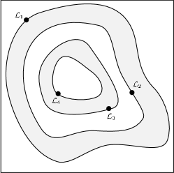
Figure 19: Cartoon illustrating (a) the posterior of a two dimensional problem; and (b) the transformed $L(X)$ function where the prior volumes $X_{i}$ are associated with each likelihood $L_{i}$.

Nested sampling [22] is a Monte Carlo technique aimed at efficient evaluation of the Bayesian evidence, but also produces posterior inferences as a by-product. It calculates the evidence by transforming the multi-dimensional evidence integral into a one–dimensional integral that is easy to evaluate numerically. This is accomplished by defining the prior volume $X$ as $dX=p(m)d^{D}m$, so that

$$X(\lambda)=\int_{L\left(m\right)>\lambda}p(m)dm,$$ (15)

where $\mathcal{L}(m)\equiv p(d|m)$ is the likelihood function and the integral extends over the region(s) of parameter space contained within the iso-likelihood contour $\mathcal{L}(m)=\lambda$. Assuming that $\mathcal{L}(X)$, i.e. the inverse of (15), is a monotonically decreasing function of $X$ (which is trivially satisfied for most posteriors), the evidence integral (3) can then be written as

$$\mathcal{Z}\equiv p(d)=\int_{0}^{1}\mathcal{L}(X){\rm d}X,$$ (16)

Thus, if one can evaluate the likelihoods $\mathcal{L}_{j}=\mathcal{L}(X_{j})$, where $X_{j}$ is a sequence of decreasing values,

$$0<X_{M}<\cdots<X_{2}<X_{1}<X_{0}=1,$$ (17)

as shown schematically in fig. 19, the evidence can be approximated numerically using standard quadrature methods as a weighted sum

$$\mathcal{Z}={\textstyle{\displaystyle\sum_{i=1}^{M}}\mathcal{L}_{i}w_{i}}.$$ (18)

In the following we will use the simple trapezium rule, for which the weights are given by $w_{i}=\frac{1}{2}(X_{i-1}-X_{i+1})$. An example of a posterior in two dimensions and its associated function $\mathcal{L}(X)$ is shown in fig. 19.

This technique allows to reduce the computational burden to about $10^{5}$ likelihood evaluations

A.1 Evidence Evaluation

The nested sampling algorithm performs the summation (18) as follows. To begin, the iteration counter is set to $i=0$ and $N$ “live” (or “active”) samples are drawn from the full prior $p(m)$ (which is often simply the uniform distribution over the prior range), so the initial prior volume is $X_{0}=1$. The samples are then sorted in order of their likelihood and the smallest (with likelihood $\mathcal{L}_{0}$) is removed from the live set and replaced by a point drawn from the prior subject to the constraint that the point has a likelihood $\mathcal{L}>\mathcal{L}_{0}$. The corresponding prior volume contained within this iso-likelihood contour will be a random variable given by $X_{1}=t_{1}X_{0}$, where $t_{1}$ follows the distribution $\Pr(t)=Nt^{N-1}$ (i.e. the probability distribution for the largest of $N$ samples drawn uniformly from the interval $[0,1]$). At each subsequent iteration $i$, the discarding of the lowest likelihood point $\mathcal{L}_{i}$ in the live set, the drawing of a replacement with $L>L_{i}$ and the reduction of the corresponding prior volume $X_{i}=t_{i}X_{i-1}$ are repeated, until the entire prior volume has been traversed. The algorithm thus travels through nested shells of likelihood as the prior volume is reduced.

The mean and standard deviation of $\log t$, which dominates the geometrical exploration, are:

$$E[\log t]=-\frac{1}{N},\qquad\sigma[\log t]=\frac{1}{N}.$$ (19)

Since each value of $\log t$ is independent, after $i$ iterations the prior volume will shrink down such that $\log X_{i}\approx-(i\pm\sqrt{i})/N$. Thus, one takes $X_{i}=\exp(-i/N)$.

A.2 Stopping Criterion

The nested sampling algorithm should be terminated on determining the evidence to some specified precision. One way would be to proceed until the evidence estimated at each replacement changes by less than a specified tolerance. This could, however, underestimate the evidence in (for example) cases where the posterior contains any narrow peaks close to its maximum. [22] provides an adequate and robust condition by determining an upper limit on the evidence that can be determined from the remaining set of current active points. By selecting the maximum-likelihood $\mathcal{L}_{\rm max}$ in the set of active points, one can safely assume that the largest evidence contribution that can be made by the remaining portion of the posterior is $\Delta{\mathcal{Z}}_{\rm i}=\mathcal{L}_{\rm max}X_{\rm i}$, i.e. the product of the remaining prior volume and maximum likelihood value. We choose to stop when this quantity would no longer change the final evidence estimate by some user-defined value (we use 0.5 in log-evidence).

A.3 Posterior Inferences

Once the evidence $\mathcal{Z}$ is found, posterior inferences can be easily generated using the full sequence of discarded points from the nested sampling process, i.e. the points with the lowest likelihood value at each iteration $i$ of the algorithm. Each such point is simply assigned the probability weight

$$p_{i}=\frac{\mathcal{L}_{i}w_{i}}{\mathcal{Z}}.$$ (20)

These samples can then be used to calculate inferences of posterior parameters such as means, standard deviations, covariances and so on, or to construct marginalised posterior distributions.

A.4 Ellipsoidal Nested Sampling

The most challenging task in implementing the nested sampling algorithm is drawing samples from the prior within the hard constraint $\mathcal{L}>\mathcal{L}_{i}$ at each iteration $i$. Employing a naive approach that draws blindly from the prior would result in a steady decrease in the acceptance rate of new samples with decreasing prior volume (and increasing likelihood).

Ellipsoidal nested sampling [55] tries to overcome the above problem by approximating the iso-likelihood contour of the point to be replaced by an $D$–dimensional ellipsoid determined from the covariance matrix of the current set of live points. New points are then selected from the prior within this (enlarged) ellipsoidal bound until one is obtained that has a likelihood exceeding that of the discarded lowest-likelihood point. In the limit that the ellipsoid coincides with the true iso-likelihood contour, the acceptance rate tends to unity.

A.5 MultiNest Algorithm

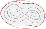
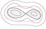
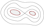
Figure 20: Cartoon of ellipsoidal nested sampling from a simple bimodal distribution. In the top left-hand panel, we see that the ellipsoid represents a good bound to the active region. Going towards the r.h.s., as we nest inward we can see that the acceptance rate will rapidly decrease as the bound steadily worsens. The final picture underneath illustrates the increase in efficiency obtained by sampling from each clustered region separately.

Ellipsoidal nested sampling as described above is efficient for simple uni-modal posterior distributions without pronounced degeneracies, but is not well suited to multi-modal distributions. As advocated by [56] and shown in fig. 20, the sampling efficiency can be substantially improved by identifying distinct clusters of live points that are well separated and constructing an individual ellipsoid for each cluster. In some problems, however, some modes of the posterior might possess a pronounced curving degeneracy so that it more closely resembles a (multi-dimensional) ‘banana’. Such features are problematic for all sampling methods, including the above mentioned clustered ellipsoidal sampling technique of [56]. To sample with maximum efficiency from such distributions, MultiNest algorithm divides the live point set into sub-clusters which are then enclosed in ellipsoids and a new point is then drawn uniformly from the region enclosed by these ‘overlapping’ ellipsoids. The no. of points in an individual sub-cluster and the total no. of sub-clusters is decided by a an ‘expectation-maximization’ algorithm so that the total sampling volume, which is equal to the sum of volumes of the ellipsoids enclosing the sub-clusters, is minimized. This allows maximum flexibility and efficiency by breaking up a mode resembling a Gaussian into relatively fewer no. of sub-clusters, and if the posterior mode possesses a pronounced curving degeneracy so that it more closely resembles a (multi-dimensional) ‘banana’ then it is broken into a relatively large no. of small ‘overlapping’ ellipsoids. The essence of this modification is illustrated in fig. 21.

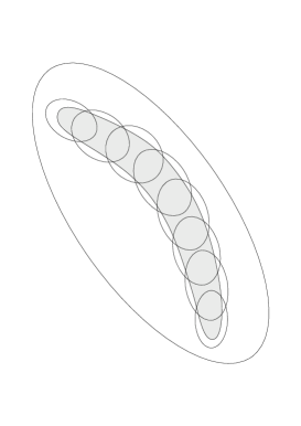
Figure 21: Cartoon of the sub-clustering approach used to deal with degeneracies. The true iso-likelihood contour contains the shaded region. The large enclosing ellipse is typical of that constructed using our basic method, whereas sub-clustering produces the set of small ellipses.

The progress of the MultiNest algorithm is controlled by two main parameters: (i) the number of live points $N$; (ii) the maximum efficiency $f$. These values can be chosen quite easily as outlined below. First, $N$ should be large enough that, in the initial sampling from the full prior space, there is a high probability that at least one point lies in the ‘basin of attraction’ of each mode of the posterior. In later iterations, live points will then tend to populate these modes. It should be remembered, of course, that $N$ must always exceed the dimensionality $D$ of the parameter space. Also, in order to calculate the evidence accurately, $N$ should be sufficiently higher so that all the regions of the parameter space are sampled adequately. The parameter $f$ controls the sampling volume $V_{i}$ at the $i^{th}$ iteration, which is equal to the sum of the volumes of the ellipoids enclosing the live point set, such that:

$$V_{i}\geq X_{i}f$$ (21)

where $X_{i}$ is the prior volume at the $i^{th}$ iteration of MultiNest algorithm and $V_{i}>X_{i}f$ in the case when at the $i^{th}$ iteration, no set of ellipsoids enclosing the $N$ live points can be found such that the sum of their volumes, $V_{i}$, is smaller than the prior volume, $X_{i}$.

For all the models analysed in this paper, we used $4,000$ live points with maximum efficiency $f$ set to $1$. This corresponds to around $500,000$ likelihood evaluations taking approximately $48$ hours on $4$ $3.0$GHz Intel Woodcrest processors.

References

-
[1]
J. R. Ellis, T. Falk, G. Ganis, K.A. Olive and M. Srednicki,
The CMSSM parameter space at large tan beta,
Phys. Lett. B 510 (2001) 236 [arXiv:hep-ph/0102098];
J. R. Ellis, K. A. Olive, Y. Santoso and V. C. Spanos, Likelihood analysis of the CMSSM parameter space, Phys. Rev. D 69 (2004) 095004 [arXiv:hep-ph/0310356];
J. R. Ellis, S. Heinemeyer, K. A. Olive and G. Weiglein, Indirect sensitivities to the scale of supersymmetry, J. High Energy Phys. 0502 (2005) 013 [arXiv:hep-ph/0411216]
-
[2]
J. R. Ellis, S. Heinemeyer, K. A. Olive and G. Weiglein,
Phenomenological indications of the scale of supersymmetry,
J. High Energy Phys. 0605 (2006) 005 [hep-ph/0602220];
- [3] O. Buchmueller et al., Predictions for Supersymmetric Particle Masses in the CMSSM using Indirect Experimental and Cosmological Constraints, arXiv:0808.4128 [hep-ph].
- [4] E. A. Baltz and P. Gondolo, Markov chain monte carlo exploration of minimal supergravity with implications for dark matter, J. High Energy Phys. 0410 (2004) 052 [hep-ph/0407039].
- [5] B. C. Allanach and C. G. Lester, Multi-dimensional MSUGRA likelihood maps, Phys. Rev. D 73 (2006) 015013 [hep-ph/0507283].
- [6] R. Ruiz de Austri, R. Trotta and L. Roszkowski, A Markov Chain Monte Carlo analysis of the CMSSM, J. High Energy Phys. 0605 (2006) 002 [hep-ph/0602028].
- [7] R. Trotta, Bayes in the sky: Bayesian inference and model selection in cosmology, Contemporary Physics, 49, 2, 71-104 (2008) [arXiv:0803.4089]
-
[8]
G. D’Agostini, Probability and Measurement Uncertainty in Physics — a Bayesian
Primer (1995) [hep-ph:/9512295];
M. Hobson, A. Jaffe, A. Liddle, P. Mukherjee et al. (Eds) Bayesian Methods in Cosmology (Cambridge University Press, Cambridge, UK, to appear, 2008). -
[9]
F. Feroz and M. P. Hobson
Multimodal nested sampling: an efficient and robust alternative to
MCMC methods for astronomical data analysis,
Mon. Not. Roy. Astron. Soc. 384 449 (2008);
F. Feroz, M. P. Hobson and M. Bridges, MultiNest: an efficient and robust Bayesian inference tool for cosmology and particle physics (2008), arXiv:0809.3437. - [10] B. C. Allanach, C. G. Lester and A. M. Weber, The dark side of mSUGRA, J. High Energy Phys. 0612 (2006) 065 [hep-ph/0609295].
- [11] L. Roszkowski, R. Ruiz de Austri and R. Trotta, On the detectability of the CMSSM light Higgs boson at the Tevatron, J. High Energy Phys. 0704 (2007) 084 [hep-ph/0611173].
- [12] L. Roszkowski, R. Ruiz de Austri and R. Trotta, Implications for the Constrained MSSM from a new prediction for , J. High Energy Phys. 0707 (2007) 075 [arXiv:0705.2012].
- [13] R. Trotta, R. Ruiz de Austri and L. Roszkowski, Prospects for direct dark matter detection in the constrained MSSM, New Astron. Rev. 51 (2007) 316 [astro-ph/0609126].
- [14] L. Roszkowski, R. Ruiz de Austri, J. Silk and R. Trotta, On prospects for dark matter indirect detection in the Constrained MSSM, arXiv:0707.0622 [hep-ph].
- [15] B. C. Allanach, M. J. Dolan and A. M. Weber, Global Fits of the Large Volume String Scenario to WMAP5 and Other Indirect Constraints Using Markov Chain Monte Carlo, arXiv:0806.1184 [hep-ph].
- [16] F. Feroz, B. C. Allanach, M. Hobson, S. S. AbdusSalam, R. Trotta and A. M. Weber, Bayesian Selection of sign(mu) within mSUGRA in Global Fits Including WMAP5 Results, J. High Energy Phys. 10 (2008) 064
- [17] B. C. Allanach, Naturalness priors and fits to the constrained minimal supersymmetric standard model, Phys. Lett. B 635 (2006) 123 [hep-ph/0601089].
- [18] B. C. Allanach, K. Cranmer, C. G. Lester, and A. M. Weber, Natural Priors, CMSSM Fits and LHC Weather Forecasts, J. High Energy Phys. 08 (2007) 023.
- [19] B. C. Allanach and D. Hooper, Panglossian Prospects for Detecting Neutralino Dark Matter in Light of Natural Priors, arXiv:0806.1923 [hep-ph].
- [20] G. L. Kane, C. F. Kolda, L. Roszkowski and J. D. Wells, Study of constrained minimal supersymmetry, Phys. Rev. D 49 (1994) 6173 [hep-ph/9312272].
- [21] R. Trotta, Mon. Not. Roy. Astron. Soc. 378 72–82 (2007).
-
[22]
J. Skilling, “Nested sampling”, in R. Fischer, R. Preuss and U. von
Toussaint (Eds) Bayesian Inference and Maximum Entropy Methods in
Science and Engineering, 735 (Amer. Inst. Phys. conf. proc. 2004),
395–405;
J. Skilling, Bayesian Analysis 1 833–861 (2006). - [23] S. Kullback and R. A. Leibler, Ann. Math. Stat. 22 79–86 (1951).
- [24] By CDF Collaboration and D0 Collaboration, A Combination of CDF and D0 Results on the Mass of the Top Quark arXiv:0803.1683 [hep-ex].
- [25] W.-M. Yao et al., The Review of Particle Physics, J. Phys. G33 (2006) 1 and 2007 partial update for the 2008 edition.
- [26] K. Hagiwara, A. D. Martin, D. Nomura and T. Teubner, Improved predictions for g-2 of the muon and , Phys. Lett. B 649 (2007) 173 [hep-ph/0611102].
- [27] K. L. Chan, U. Chattopadhyay and P. Nath, Naturalness, weak scale supersymmetry and the prospect for the observation of supersymmetry at the Tevatron and at the LHC, Phys. Rev. D 58 (1998) 096004 [hep-ph/9710473].
- [28] J. L. Feng, K. T. Matchev and T. Moroi, Multi - TeV scalars are natural in minimal supergravity, Phys. Rev. Lett. 84 (2000) 2322 [hep-ph/9908309] and Focus points and naturalness in supersymmetry, Phys. Rev. D 61 (2000) 075005 [hep-ph/9909334].
-
[29]
See, e.g., H. P. Nilles,
Supersymmetry, Supergravity and Particle Physics,
Phys. Rept. 110 (1984) 1;
A. Brignole, L. E. Ibañez and C. Muñoz, Soft supersymmetry breaking terms from supergravity and superstring models, published in Perspectives on Supersymmetry, ed. G. L. Kane, 125 [hep-ph/9707209]. - [30] See http://lepewwg.web.cern.ch/LEPEWWG.
- [31] J. P. Miller, E. de Rafael and B. L. Roberts, Muon g-2: Review of Theory and Experiment, Rept. Prog. Phys. 70 (2007) 795 [arXiv:hep-ph/0703049].
- [32] Heavy Flavor Averaging Group (HFAG) (E. Barberio et al.), Averages of b-hadron properties at the end of 2006, arXiv:0704.3575 [hep-ex].
- [33] The CDF Collaboration, Measurement of the oscillation frequency, Phys. Rev. Lett. 97 (2006) 062003 [hep-ex/0606027] and Observation of oscillations, Phys. Rev. Lett. 97 (2006) 242003 [hep-ex/0609040].
- [34] J. Dunkley et al. [The WMAP Collaboration], Five-year Wilkinson Microwave Anisotropy Probe (WMAP) Observations: Likelihoods and parameters from the WMAP data, arXiv:0803.0586 [astro-ph].
- [35] The CDF Collaboration, Search for and decays in collisions with CDF-II, CDF note 8956 (August 2007).
-
[36]
The LEP Higgs Working Group,
http://lephiggs.web.cern.ch/LEPHIGGS;
G. Abbiendi et al. [the ALEPH Collaboration, the DELPHI Collaboration, the L3 Collaboration and the OPAL Collaboration, The LEP Working Group for Higgs Boson Searches], Search for the standard model Higgs boson at LEP, Phys. Lett. B 565 (2003) 61 [hep-ex/0306033]. - [37] M. Awramik, M. Czakon, A. Freitas and G. Weiglein, Precise prediction for the W boson mass in the standard model, Phys. Rev. D 69 (2004) 053006 [hep-ph/0311148]; and Complete two-loop electroweak fermionic corrections to and indirect determination of the Higgs boson mass, Phys. Rev. Lett. 93 (2004) 201805 [hep-ph/0407317].
- [38] A. Djouadi, P. Gambino, S. Heinemeyer, W. Hollik, C. Junger and G. Weiglein, Leading QCD corrections to scalar quark contributions to electroweak precision observables, Phys. Rev. D 57 (1998) 4179 [hep-ph/9710438].
- [39] See http://www.ippp.dur.ac.uk/old/MuonMDM/ for a recent collection of results.
- [40] M. Misiak and M. Steinhauser, NNLO QCD corrections to the matrix elements using interpolation in , Nucl. Phys. B 764 (2007) 62 [hep-ph/0609241].
- [41] M. Misiak et al., Estimate of at , Phys. Rev. Lett. 98 (2007) 022002, [hep-ph/0609232].
- [42] C. Degrassi, P. Gambino and G. F. Giudice, in supersymmetry: large contributions beyond the leading order, J. High Energy Phys. 0012 (2000) 009 [hep-ph/0009337].
- [43] P. Gambino and M. Misiak, Quark mass effects in , Nucl. Phys. B 611 (2001) 338 [hep-ph/0104034].
- [44] K. Okumura and L. Roszkowski, Deconstraining supersymmetry from , Phys. Rev. Lett. 92 (2004) 161801 [hep-ph/0208101]; Large beyond leading order effects in in supersymmetry with general flavour mixing, J. High Energy Phys. 0310 (2003) 024 [hep-ph/0308102].
- [45] J. Foster, K. Okumura and L. Roszkowski, New Higgs effects in B–physics in supersymmetry with general flavour mixing, Phys. Lett. B 609 (2005) 102 [hep-ph/0410323] and Probing the flavour structure of supersymmetry breaking with rare B–processes: a beyond leading order analysis, J. High Energy Phys. 0508 (2005) 094 [hep-ph/0506146].
- [46] A. Gray et al. [HPQCD Collaboration], The B meson decay constant from unquenched lattice QCD, Phys. Rev. Lett. 95 (2005) 212001 [hep-lat/0507015].
- [47] The Unitarity Triangle Fit Collaboration, http://www.utfit.org.
- [48] G. Belanger, F. Boudjema, A. Pukhov and A. Semenov, MicrOMEGAs: A program for calculating the relic density in the MSSM, Comput. Phys. Commun. 149 (2002) 103 [hep-ph/0112278]; MicrOMEGAs: Version 1.3, Comput. Phys. Commun. 174, 577 (2006) [hep-ph/0405253].
- [49] J. Foster, K. Okumura and L. Roszkowski, Current and future limits on general flavor violation in transitions in minimal supersymmetry, J. High Energy Phys. 0603 (2006) 044 [hep-ph/0510422] and New Constraints on SUSY Flavour Mixing in Light of Recent Measurements at the Tevatron, Phys. Lett. B 641 (2006) 452 [hep-ph/0604121].
- [50] Z. Ahmed et al. [CDMS Collaboration], A Search for WIMPs with the First Five-Tower Data from CDMS, arXiv:0802.3530 [astro-ph].
- [51] J. Angle et al. [XENON Collaboration], First Results from the XENON10 Dark Matter Experiment at the Gran Sasso National Laboratory, Phys. Rev. D 100 (2008) 021303 [arXiv:0706.0039 [astro-ph]].
- [52] G. J. Alner et al., First limits on WIMP nuclear recoil signals in ZEPLIN-II: A two phase xenon detector for dark matter detection,’, Astropart. Phys. 28 (2007) 287 [arXiv:astro-ph/0701858].
- [53] J. Ellis, K.A. Olive and C. Savage Hadronic Uncertainties in the Elastic Scattering of Supersymmetric Dark Matter arXiv:0801.3656.
- [54] B.C. Allanach, private communication.
- [55] P. Mukherjee, D. Parkinson and A. R. Liddle, A Nested Sampling Algorithm for Cosmological Model Selection, Astrophys. J. 638 (2006) L51 [astro-ph/0508461].
- [56] R. Shaw, M. Bridges and M. P. Hobson, Clustered nested sampling: efficient Bayesian inference for cosmology, Mon. Not. Roy. Astron. Soc. 378, 1365 (2007) [astro-ph/0701867].