Ballistic transport in disordered graphene

Abstract

An analytic theory of electron transport in disordered graphene in a ballistic geometry is developed. We consider a sample of a large width $W$ and analyze the evolution of the conductance, the shot noise, and the full statistics of the charge transfer with increasing length $L$, both at the Dirac point and at a finite gate voltage. The transfer matrix approach combined with the disorder perturbation theory and the renormalization group is used. We also discuss the crossover to the diffusive regime and construct a “phase diagram” of various transport regimes in graphene.

I Introduction

Recent successes in manufacturing of atomically thin graphite samples Novoselov04 ; NovoselovPNAS ; Novoselov05 ; Zhang05 (graphene) have stimulated intense experimental and theoretical activity Geim07 ; RMP07 . The key feature of graphene is the massless Dirac type of low-energy electron excitations. This gives rise to a number of remarkable physical properties of this system distinguishing it from conventional two-dimensional metals. One of the most prominent features of graphene is the “minimal conductivity” at the neutrality (Dirac) point. Specifically, the conductivityNovoselov05 ; Zhang05 ; Kim of an undoped sample is close to $e^{2}/h$ per spin per valley, remaining almost constant in a very broad temperature range — from room temperature down to 30mK.

Several recent theoretical works addressed transport in disordered graphene samples. It was found that localization properties depend strongly on the nature of disorder Aleiner06 ; McCann ; Altland06 ; OurPRB ; OurPRL ; OurEPJ ; OurQHE which determines the symmetry and topology of the corresponding field theory. The localization is absent provided a certain symmetry of clean graphene Hamiltonian is preserved in the disordered sample, see Ref. OurEPJ, .

One possibility is that disorder preserves a chiral symmetry of massless Dirac fermions. This situation is, in particular, realized when the dominant disorder is due to corrugations of graphene sheet (ripples) and/or dislocations. GuineaMorpurgo The conductivity in such chiral-symmetric models has been shown OurPRB to be exactly $e^{2}/\pi h$ (per spin per valley) at the Dirac point. While being temperature independent, this value is, however, less by a factor of $\sim 3$ than the experimentally measured values.

Another possibility, a long-range randomness, was studied in Ref. OurPRL, . This type of disorder does not mix the two valleys of the graphene spectrum, which leads to emergence of a topological term in the corresponding field theory (unitary or symplectic $\sigma$-model). The peculiar topological properties protect the system from localization OurPRL ; OurEPJ ; OurQHE ; Ryu07 ; Koshino07 . It is worth mentioning that a topologically protected metallic state emerging in graphene with long-range random potential also arises at a surface of a three-dimensional $Z_{2}$ topological insulator. Hasan08 ; Schnyder08

A number of numerical simulations of electron transport in disordered graphene Nomura07 ; Rycerz07 ; Bardarson07 ; Koshino07 ; San-Jose07 ; Lewenkopf08 confirmed the absence of localization in the presence of long-range random potential. The main quantity studied numerically in most of these works is the conductance $G$ of a finite-size graphene sample with a width $W$ much larger than the length $L$. This setup allows one to define the “conductivity” $\sigma\equiv GL/W$ even for ballistic samples with $L$ much shorter than the mean free path $l$. Remarkably, in graphene at the Dirac point, such ballistic “conductivity” has a universal value $e^{2}/\pi h$ in the clean case. Katsnelson06 ; Tworzydlo06 This setup was studied experimentally in Refs. Morpurgo06, ; Miao07, ; Danneau07, ; Danneau08, and the ballistic value $e^{2}/\pi h$ was indeed observed for large aspect ratios. This geometry of samples is particularly advantageous for the analysis of evolution from the ballistic to diffusive transport.

A complete description of the electron transport through a finite system involves not only the conductance but also higher cumulants of the distribution of transferred charge. The second moment is related to the current noise in the system. The intensity of the shot noise is characterized by the Fano factor $F$. For clean graphene, this quantity was studied in Ref. Tworzydlo06, . Surprisingly, in a short and wide sample ($W\gg L$) the Fano factor takes the universal value $F=1/3$, that coincides with the well-known result for a diffusive metallic wire. BeenakkerRMP This is at odds with usual clean metallic systems, where the shot noise is absent ($F=0$). The Fano factor $F=1/3$ in clean graphene is attributed Tworzydlo06 to the fact that the current is mediated by evanescent rather than propagating modes. Furthermore, the whole distribution of transmission eigenvalues for the massless Dirac equation in a clean sample with $W\gg L$ at the Dirac point agrees with that of mesoscopic metallic wires in the diffusive regime. Ludwig07

The effect of disorder on the shot noise was studied numerically in Refs. San-Jose07, ; Lewenkopf08, , where the value of the Fano factor $F\approx 0.3$ was found across the whole crossover form ballistics to diffusion. The Fano factor close to $1/3$ was also observed at the Dirac point experimentally. Danneau07 ; Danneau08 When the chemical potential was shifted away from the Dirac point, the Fano factor decreased, then showed an intermediate shoulder at $F\approx 0.15$, and finally approached zero for largest gate voltages (carrier concentrations).

While both diffusive and clean limits have been addressed analytically, only numerical and experimental results for the intermediate regime of ballistic transport through disordered samples have been available so far.foot-1D The aim of this paper is to fill this gap. We develop the analytic theory of electron transport in disordered graphene in the ballistic geometry ($L\ll W,l$) and calculate the full statistics of the charge transfer for both zero (the Dirac point) and large concentration of carriers. We also discuss the crossover to diffusive regime and construct the overall “phase diagram” of transport regimes.

The structure of the paper is as follows. We begin in Sec. II with the introduction of the model and derivation of a general transfer-matrix equation. In Sec. III we calculate transport properties of a clean sample. In Sec. IV the disorder is included in the lowest order of the perturbation theory. The resummation of leading higher-order corrections to the counting statistics is performed within the renormalization group approach in Sec. V. For the case of random potential we present an evidence in favor of a universal scaling of the distribution function of transmission coefficients valid at the Dirac point for samples of arbitrary size (covering both ballistic and diffusive regimes). We summarize the results and discuss the perspectives in Sec. VI. Technical details are relegated to Appendices A, B, and C.

II Transfer-matrix technique

We start with introducing our model and the general formalism of transfer matrix technique. For graphene, this approach was employed in Refs. Katsnelson06, ; Tworzydlo06, ; Titov06, ; CheianovFalko, ; Titov07, ; San-Jose07, .

We will adopt the single-valley model of graphene. More specifically, we will consider scattering of electrons only within a single valley and neglect intervalley scattering events. Indeed, a number of experimental results show that the dominant disorder in graphene scatters electrons within the same valley. First, this disorder model is supported by the odd-integer quantizationNovoselov05 ; Zhang05 ; Geim07 of the Hall conductivity, $\sigma_{xy}=(2n+1)2e^{2}/h$, representing a direct evidenceOurQHE in favor of smooth disorder which does not mix the valleys. The analysis of weak localization also corroborates the dominance of intra-valley scatteringSavchenko . Furthermore, the observation of the linear density dependenceGeim07 of graphene conductivity away from the Dirac point implies that the relevant disorder is due to charged impurities and/or ripples.Nomura07 ; Ando06 ; Nomura06 ; Khveshchenko ; OurPRB ; footnote-unitary Due to the long-range character of these types of disorder, the intervalley scattering amplitudes are strongly suppressed and will be neglected in our treatment. Finally, apparent absence of localization at the Dirac point down to very low temperaturesNovoselov05 ; Zhang05 ; Kim can be explained only by some special symmetry of disorder. The most realistic candidate model is the long-range randomness which does not scatter between valleys. OurPRL

The single-valley massless Dirac Hamiltonian of electrons in graphene has the form (see, e.g., Ref. RMP07, )

$$H=v_{0}\bm{\sigma}\mathbf{p}+V(x,y),\qquad V(x,y)=\sigma_{\mu}V_{\mu}(x,y).$$ (1)

Here $\sigma_{\mu}$ (with $\mu=0,x,y,z$) are Pauli matrices acting on the electron pseudospin degree of freedom corresponding to the sublattice structure of the honeycomb lattice, $\bm{\sigma}\equiv\{\sigma_{x},\sigma_{y}\}$, and the Fermi velocity is $v_{0}\approx 10^{8}$ cm/s. The random part $V(x,y)$ is in general a $2\times 2$ matrix in the sublattice space. Below we set $\hbar=1$ and $v_{0}=1$ for convenience.

We will calculate transport properties of a rectangular graphene sample with the dimensions $L\times W$. The contacts are attached to the two sides of the width $W$ separated by the distance $L$. We fix the $x$ axis in the direction of current, Fig. 1, with the contacts placed at $x=0$ and $x=L$. We assume $W\gg L$, which allows us to neglect the boundary effects related to the edges of the sample that are parallel to the $x$ axis (at $y=\pm W/2$).

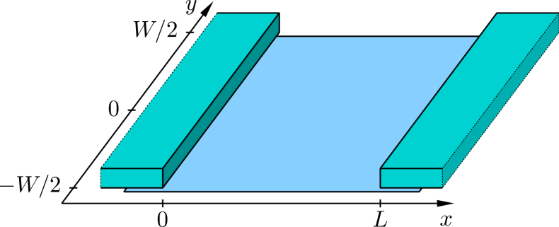
Figure 1: (Color online) Schematic setup for two-terminal transport measurements. Graphene sample of dimensions $L\times W$ is placed between two parallel contacts. We assume $W\gg L$ throughout the paper.

Following Ref. Tworzydlo06, , metallic contacts are modelled as highly doped graphene regions described by the same Hamiltonian (1). In other words, we assume that the chemical potential $E_{F}$ in the contacts is shifted far from the Dirac point. In particular, $E_{F}\gg\epsilon$, where $\epsilon$ is the chemical potential inside the graphene sample counted from the Dirac point. (All our results are independent of the sign of energy, thus we assume $\epsilon>0$ throughout the paper.) A large number of propagating modes exists in the leads, all belonging to the circular Fermi surface of radius $p_{F}=E_{F}/v_{0}$. These modes are labelled by the momentum $p_{n}=2\pi n/W$ in $y$ direction with $|n|<N=Wp_{F}/2\pi$. Particular boundary conditions at $y=\pm W/2$ shift the quantized values of $p_{n}$ by a constant of order $1/W$. However, this constant has no significance in the limit $W\gg L$ when many channels participate in electron transport.

Clearly, the transverse momentum $p_{n}$ is preserved in the clean system. We will use the mixed momentum-coordinate representation, with the wave function $\Psi_{n}(x)$ bearing a vector index $n$ in the space of transverse momenta supplemented by a 2-spinor structure in pseudospin (sublattice) space. The eigenstates of the clean Hamiltonian $H_{0}=v_{0}\bm{\sigma}\mathbf{p}$ have the direction of pseudospin parallel to the electron momentum. It is convenient to perform the unitary rotationTitov07 in the pseudospin space $\psi=\mathcal{L}\Psi$ with $\mathcal{L}=(\sigma_{x}+\sigma_{z})/\sqrt{2}$ which transforms $\sigma_{x}$ to the diagonal form: $\mathcal{L}\sigma_{x}\mathcal{L}^{\dagger}=\sigma_{z}$. Hence the two components of the rotated spinor correspond to right- and left-propagating waves, footnote-EFinLeads $\psi=\{\psi^{R},\psi^{L}\}$. In terms of the new function $\psi_{n}(x)$, the Schrödinger equation $H\Psi=\epsilon\Psi$ acquires the form San-Jose07 ; Titov07

$$\frac{\partial\psi_{n}}{\partial x}=(\sigma_{x}p_{n}+i\sigma_{z}\epsilon)\psi_{n}-i\sigma_{z}\sum_{m}U_{nm}(x)\psi_{m}.$$ (2)

The matrix $U_{nm}(x)$ represents the operator $\mathcal{L}V(x,y)\mathcal{L}^{\dagger}$ in the mixed momentum-coordinate representation

$$U_{nm}(x)=\int\frac{dy}{W}\,e^{-i(p_{n}-p_{m})y}\mathcal{L}V(x,y)\mathcal{L}^{\dagger}.$$ (3)

A standard description of electron propagation involves the scattering matrix $\mathcal{S}$. This is a unitary matrix relating the amplitudes of incident and outgoing waves

$$\begin{pmatrix}\psi^{L}(0)\\ \psi^{R}(L)\end{pmatrix}=\mathcal{S}\begin{pmatrix}\psi^{R}(0)\\ \psi^{L}(L)\end{pmatrix},\qquad\mathcal{S}=\begin{pmatrix}r&t^{\prime}\\ t&r^{\prime}\end{pmatrix}.$$ (4)

The elements $t$, $t^{\prime}$ and $r$, $r^{\prime}$ are matrices in channel space formed by transmission and reflection amplitudes, respectively. The unitarity condition $\mathcal{S}^{\dagger}\mathcal{S}=\mathbb{1}$ ensures conservation of particle number.

A closely related formulation is based on the transfer matrix $\mathcal{T}$ which expresses the waves at the point $x=L$ through those at $x=0$:

$$\begin{pmatrix}\psi^{R}(L)\\ \psi^{L}(L)\end{pmatrix}=\mathcal{T}\begin{pmatrix}\psi^{R}(0)\\ \psi^{L}(0)\end{pmatrix},\quad\mathcal{T}=\begin{pmatrix}{t^{\dagger}}^{-1}&r^{\prime}{t^{\prime}}^{-1}\\ -{t^{\prime}}^{-1}r&{t^{\prime}}^{-1}\end{pmatrix}.$$ (5)

This description is convenient due to the simple multiplicativity property: $\mathcal{T}(x_{3},x_{2})\mathcal{T}(x_{2},x_{1})=\mathcal{T}(x_{3},x_{1})$. The current conservation is provided by the identity $\mathcal{T}^{\dagger}\sigma_{z}\mathcal{T}=\sigma_{z}$.

By definition, the transfer matrix $\mathcal{T}(x_{2},x_{1})$ yields a solution to the Schrödinger equation (2) in the form $\psi(x_{2})=\mathcal{T}(x_{2},x_{1})\psi(x_{1})$. Transfer matrix itself, as a function of its first argument, obeys the same Schrödinger equation with the initial condition $\mathcal{T}(x,x)=\mathbb{1}$. In a clean sample the solution depends only on the difference $x_{2}-x_{1}$ and is diagonal in channel space:

$$\mathcal{T}^{(0)}_{nm}(x_{2},x_{1})=\delta_{nm}\exp\bigl{[}(\sigma_{x}p_{n}+i\sigma_{z}\epsilon)(x_{2}-x_{1})\bigr{]}.$$ (6)

In order to include disorder as a perturbation, it is convenient to cast the Schrödinger equation (2) into an integral form. In terms of transfer matrix the integral equation reads

$$\mathcal{T}(x_{2},x_{1})=\mathcal{T}^{(0)}(x_{2},x_{1})\\ -i\int_{x_{1}}^{x_{2}}dx\,\mathcal{T}^{(0)}(x_{2},x)\sigma_{z}U(x)\mathcal{T}(x,x_{1}).$$ (7)

The transport statistics of the sample is expressed in terms of transmission eigenvalues $T_{n}$ — the eigenvalues of the matrix $t^{\dagger}t$. One can extract these transmission eigenvalues from the upper left element of the transfer matrix (5). The first two moments of the transferred charge distribution determine the conductance (by Landauer formula) and the Fano factor BeenakkerRMP

$$G=\frac{4e^{2}}{h}\mathop{\mathrm{Tr}}(t^{\dagger}t),\qquad F=1-\frac{\mathop{\mathrm{Tr}}(t^{\dagger}t)^{2}}{\mathop{\mathrm{Tr}}(t^{\dagger}t)}.$$ (8)

The factor $4$ in the expression for the conductance accounts for the spin and valley degeneracy.

III Clean graphene

We will first analyze transport properties of a clean graphene strip. In the “short and wide” geometry ($W\gg L$) we are considering, the total number of channels participating in charge transfer is large. This allows us to replace summation over channels by integration. From now on, we will identify channels by the dimensionless momentum $p=p_{n}L$ in $y$ direction and integrate over this momentum according to

$$\sum_{n}\mapsto\frac{W}{L}\int\frac{dp}{2\pi}.$$ (9)

The transfer matrix $\mathcal{T}^{(0)}$, and hence its upper-left block ${t^{\dagger}}^{-1}$, are diagonal in channels. Using the explicit form of the clean graphene transfer matrix, Eq. (6), one calculates the transmission eigenvalues Titov07

$$T_{p}=(t^{\dagger}t)_{pp}=\left[1+\frac{p^{2}\sinh^{2}\sqrt{p^{2}-(\epsilon L)^{2}}}{p^{2}-(\epsilon L)^{2}}\right]^{-1}.$$ (10)

For the conductance and Fano factor we obtain from Eq. (8)

$$G=\frac{2e^{2}W}{\pi hL}\int dp\;T_{p},\qquad F=1-\frac{\int dp\;T_{p}^{2}}{\int dp\;T_{p}}.$$ (11)

The result of numerical integration of Eq. (11) is shown in Fig. 2. A detailed analytical analysis of the two limiting cases of small and large energies is presented below.

Figure 2: Energy dependence of the (a) conductance and the (b) Fano factor of the clean sample with $W\gg L$. Solid lines show numerical results. Low energy asymptotics Eq. (20) is plotted by dashed lines while dotted lines correspond to high energy limit Eqs. (33) and (34). Asymptotical curves provide a very good approximation to the exact result in the whole range of energies.

III.1 Transmission distribution and counting statistics

It is convenient to introduce the distribution function $P(T)$ of transmission eigenvalues (10). This distribution function provides a measure in the space of channels which is, by definition, equivalent to the integration measure (9),

$$P(T)\,dT=\frac{W\,d|p|}{\pi L}.$$ (12)

According to (10), there is one-to-one correspondence between the transmission eigenvalue $0\leq T\leq 1$ and the absolute value $|p|$ of the momentum; an extra factor of $2$ in the right-hand side of Eq. (12) accounts for the double degeneracy between channels with momenta $p$ and $-p$.

Very generally, the distribution function $P(T)$ determines the full statistics of the charge transfer. Specifically, one defines the counting statistics $\kappa(\chi)=\sum_{N}e^{i\chi N}\mathcal{P}(N)$, where $\mathcal{P}(N)$ is the probability that $N$ particles are transferred within a measurement time interval $t_{m}$. Then $\ln\kappa(\chi)$ is the generating function for cumulants,

$$\ln\kappa(\chi)=\sum_{k}\frac{(i\chi)^{k}}{k!}\langle\langle N^{k}\rangle\rangle.$$ (13)

It can be related to $P(T)$ in the following way LeeLevitovYakovets (we assume zero temperature and retain the factor of 4 taking into account the spin and valley degeneracy in graphene):

$$\ln\kappa(\chi)=\frac{4e^{2}}{h}Vt_{m}\int dTP(T)\ln(1-T+e^{i\chi}T),$$ (14)

where $V$ is the applied voltage. In particular, the first two of the cumulants $\langle\langle N^{k}\rangle\rangle$ determine the conductance $G$ and the shot noise power $S$ via $\langle\langle N\rangle\rangle\equiv\langle N\rangle=Vt_{m}G$ and $\langle\langle N^{2}\rangle\rangle=Vt_{m}S$. According to Eqs. (13), (14), one has

$$G=\frac{4e^{2}}{h}\int dT\,TP(T),\qquad S=\frac{4e^{2}}{h}\int dT\,T(1-T)P(T),$$ (15)

and the Fano factor

$$F=\frac{S}{G}=1-\frac{\int dT\,T^{2}P(T)}{\int dT\,TP(T)}.$$ (16)

The relations (14), (15), (16) are of general validity and equally applicable to the clean and disordered system. All the information about scattering, both at the interface with leads and in the bulk of the system, is encoded in the transmission distribution $P(T)$. Clearly, Eqs. (15), (16) for the conductance and the shot noise are equivalent to Eq. (8).

III.2 Low energies: $\epsilon L\ll 1$

In the low energy limit, we calculate the distribution function $P(T)$ in the form of a power series in the small parameter $\epsilon L$. In order to perform this calculation, we first invert the function $T_{p}$ given by Eq. (10) keeping terms of the second order in $\epsilon L$:

$$p(T)=p_{0}(T)+\frac{(\epsilon L)^{2}}{2}\left[\frac{1}{p_{0}(T)}-\frac{\sqrt{1-T}}{p_{0}^{2}(T)}\right],$$ (17)

$$p_{0}(T)=\mathop{\mathrm{arccosh}}\frac{1}{\sqrt{T}}.$$ (18)

Now we substitute this expression into Eq. (12) and obtain the distribution

$$P(T)=\frac{W}{\pi L}\,\frac{dp(T)}{dT}\\ =\frac{W}{2\pi L}\frac{1}{T\sqrt{1-T}}\left[1+(\epsilon L)^{2}\left(\frac{\sqrt{1-T}}{p_{0}^{3}(T)}-\frac{1+T}{2p_{0}^{2}(T)}\right)\right].$$ (19)

It is worth noticing that by definition $\int dTP(T)$ should give the total number of open channels $Wp_{F}/\pi$ in the leads. In fact, the logarithmic divergence at $T\to 0$ of the normalization of Eq. (19) is cut off at the lowest transmission eigenvalue $T_{\rm min}\sim\exp(-2p_{F}L)$. This small-$T$ cutoff is, however, immaterial for the calculation of the moments (conductance, noise, etc).

At zero energy, the function $P(T)$ reproduces the well-known Dorokhov result Dorokhov83 for a diffusive wire. This is, in particular, the reason for the $1/3$ Fano factor in graphene. Tworzydlo06 The fact that the clean graphene sample is characterized by exactly the same form of the transmission distribution as a generic diffusive wire is highly nontrivial. We will show below (Secs. IV and V) that this remarkable correspondence remains valid in the ballistic regime when leading disorder effects are incorporated.

Using the distribution (19), we obtain the following results for the conductance and the Fano factor of clean graphene at low energies, $\epsilon L\ll 1$,

$$G =\frac{4e^{2}}{\pi h}\;\frac{W}{L}\left[1+c_{1}(\epsilon L)^{2}\right],\quad F=\frac{1}{3}\left[1+c_{2}(\epsilon L)^{2}\right],$$ (20)

$$c_{1} =\frac{35\zeta(3)}{3\pi^{2}}-\frac{124\zeta(5)}{\pi^{4}}\approx 0.101,$$ (21)

$$c_{2} =-\frac{28\zeta(3)}{15\pi^{2}}-\frac{434\zeta(5)}{\pi^{4}}+\frac{4572\zeta(7)}{\pi^{6}}\approx-0.052.$$ (22)

At the Dirac point ($\epsilon=0$), Eq. (20) reproduces the earlier analytical results of Refs. Katsnelson06, ; Tworzydlo06, . Low energy asymptotics is shown with dashed lines in Fig. 2.

III.3 High energies: $\epsilon L\gg 1$

When the Fermi energy $\epsilon$ in the sample is far from the Dirac point, many conducting ($T\sim 1$) channels are opened. In this regime, the conductivity and higher moments of the transmission distribution are essentially linear in $\epsilon$ with small oscillating corrections (see Fig. 2). These oscillations are due to interference effects: conductance is relatively enhanced and the noise is suppressed when a channel exhibits resonant transmission with $T$ close to $1$. This phenomenon is similar to the Fabry-Perot resonances.

We begin with the calculation of the main (proportional to $\epsilon$) part of the transmission distribution function and will return to the oscillatory correction later in this section. It is convenient to find first the generating function of transmission moments, defined as

$$\mathcal{F}(z)=\sum_{n=1}^{\infty}z^{n-1}\mathop{\mathrm{Tr}}(t^{\dagger}t)^{n}=\mathop{\mathrm{Tr}}\left[t^{-1}{t^{\dagger}}^{-1}-z\right]^{-1}.$$ (23)

This function appears to be very useful for the forthcoming calculation of the transport properties of a disordered sample. In this section, we apply it to the clean system. According to Eqs. (23) and (10), we have

$$\mathcal{F}(z)=\frac{W}{L}\int\frac{dp}{2\pi}\left[1-z+\frac{p^{2}\sin^{2}\sqrt{(\epsilon L)^{2}-p^{2}}}{(\epsilon L)^{2}-p^{2}}\right]^{-1}.$$ (24)

The integrand oscillates rapidly in the interval $-\epsilon L<p<\epsilon L$. This interval of momenta contains all open (well-conducting) channels and thus provides the main contribution to the generating function. At high energies, it is convenient to introduce a new variable $u$, such that

$$p=p_{n}L=\epsilon L\sqrt{1-u^{2}},$$ (25)

$$\int dpf(p) \mapsto \epsilon L\int_{0}^{1}\frac{u\,du}{\sqrt{1-u^{2}}}$$

$$\times \bigl{[}f(\epsilon L\sqrt{1-u^{2}})+f(-\epsilon L\sqrt{1-u^{2}})\bigr{]}.$$

Transforming Eq. (24) to the new variable (25) and averaging over oscillations (see Appendix A for details), we obtain

$$\mathcal{F}(z)=\frac{W\epsilon}{\pi\sqrt{1-z}}\int_{0}^{1}\frac{u^{2}\,du}{\sqrt{1-u^{2}}\sqrt{1-zu^{2}}}\\ =\frac{W\epsilon}{\pi}\,\frac{K(z)-E(z)}{z\sqrt{1-z}}.$$ (27)

Here $K(m)$ and $E(m)$ are complete elliptic integrals of the first and second kind footnote-elliptic with the parameter $m$.

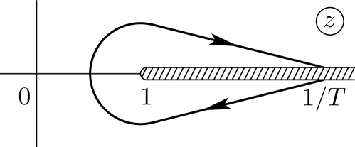
Figure 3: Integration contour used in Eq. (29).

The function $\mathcal{F}(z)$ is regular at the point $z=0$. The coefficients of the series expansion near this point provide the moments of transferred charge distribution, see Eq. (23). The transmission distribution function $P(T)$ is related to $\mathcal{F}(z)$ by the linear integral equation

$$\int_{0}^{1}\frac{P(T)}{T^{-1}-z}\,dT=\mathcal{F}(z),$$ (28)

which follows from Eq. (23). In order to solve this equation for $P(T)$, we note that the function $\mathcal{F}(z)$ has a branch cut along real axis running from $1$ to $\infty$. We integrate Eq. (28) along a contour going from $z=1/T-i0$ to $z=1/T+i0$ encircling the point $z=1$, see Fig. 3. This integration yields

$$\int\limits_{1/T-i0}^{1/T+i0}\frac{dz}{2\pi i}\,\mathcal{F}(z)=\int_{0}^{1}P(\tilde{T})d\tilde{T}\int\limits_{1/T-i0}^{1/T+i0}\frac{dz}{2\pi i({\tilde{T}}^{-1}-z)}\\ =\int_{T}^{1}P(\tilde{T})d\tilde{T}.$$ (29)

To find the distribution function, we calculate the derivative of the above equation with respect to $T$ and obtain

$$P(T)=\frac{\mathcal{F}(1/T+i0)-\mathcal{F}(1/T-i0)}{2\pi iT^{2}}.$$ (30)

This identity establishes a relation between the distribution function $P(T)$ and the jump of $\mathcal{F}(z)$ across the branch cut at the point $z=1/T$. In other words, equation (28) solves the corresponding Riemann-Hilbert problem.

To find the explicit formula for the distribution $P(T)$, we perform an analytic continuation of the expression (27) from the vicinity of the point $z=0$ to $z=1/T\pm i0$ and substitute the result into Eq. (30). This yields

$$P(T)=\frac{W\epsilon}{\pi^{2}}\;\frac{K(T)-E(T)}{T\sqrt{1-T}}.$$ (31)

This distribution function provides a full transport description at high energies (up to small oscillatory corrections discussed below). We note that Eq. (31) does not take into account almost closed (evanescent) channels with $p_{n}>\epsilon$ (and thus $T\ll 1$). Estimating their contribution, we find that it is suppressed by a factor $(\epsilon L)^{-4}$ compared to the main term, thus yielding a negligible contribution to the charge transfer.

Using the above distribution (or, equivalently, the generating function), we calculate the asymptotics of the conductance and Fano factor in the high-energy limit $\epsilon L\gg 1$,

$$G=\frac{e^{2}}{h}\;W\epsilon,\qquad\qquad F=\frac{1}{8}.$$ (32)

We recall that when passing from Eq. (24) to Eq. (27), we neglected the oscillatory contributions to the generating function. A more accurate calculation accounting for these oscillations is presented in Appendix A [see Eq. (130)]. The results for the conductance and the Fano factor read

$$G =\frac{e^{2}}{h}\;W\epsilon\left[1+\frac{\sin(2\epsilon L-\pi/4)}{2\sqrt{\pi}(\epsilon L)^{3/2}}\right],$$ (33)

$$F =\frac{1}{8}\left[1-\frac{9\sin(2\epsilon L-\pi/4)}{2\sqrt{\pi}(\epsilon L)^{3/2}}\right].$$ (34)

These results are in a good agreement with the high-energy behavior of $G$ and $F$ calculated numerically, see Fig. 2.

Let us emphasize that transport properties of the system at high energies depend on the particular model of the contacts. Schomerus07 ; Blanter07 In our calculation we assume that the boundaries between graphene and the leads are sharp. This model is well justified if the actual extension $d$ of the transitional region at the interface is small compared to the electron wavelength in graphene. This wavelength is energy dependent: it tends to infinity at $\epsilon=0$ and decreases with increasing $\epsilon$. Thus the small-energy results, Sec. III.2, are universal and not influenced by the microscopic details of the interface provided the size of the boundary transitional region is much smaller than the length of the sample $L$. On the other hand, the results of the current section are applicable for not too high energies, $\epsilon\ll 1/d$. For higher energy, the electron wavelength becomes comparable to $d$ and the transmission properties of the sample become nonuniversal. In the extreme high-energy limit, $\epsilon d\gg 1$ the boundary becomes adiabatically smooth. This, in particular, leads to the vanishing Fano factor because the semiclassically propagating electrons are either transmitted or reflected without any uncertainty.

Our results for the energy dependence of the conductance and the Fano factor in clean graphene are in agreement with the findings of Refs. Tworzydlo06, ; Titov07, , where the sum over transmission channels was evaluated numerically for a finite (but sufficiently large) ratio $W/L$. Experimentally, such a ballistic setup was studied in Refs. Danneau07, ; Danneau08, . Most of the experimental observations reasonably agree with our results. The “conductivity” $GL/W$ (which is equal to $4e^{2}/\pi h$ at the neutrality point, as expected for a ballistic sample) increases roughly linearly with energy $\epsilon$. The Fano factor has a value close to $1/3$ at the Dirac point and decreases when one moves away from the Dirac point, showing a tendency to saturate at $F\approx 0.15$, which is not far from the value 1/8 we have obtained in the high-energy regime. Measurements on other samples reveal that very far from the Dirac point the Fano factor decreases again, reaching a value as low as 0.02. Apparently, the intermediate plateau corresponds to the high-energy regime $L^{-1}\ll\epsilon\ll d^{-1}$ investigated in our work, while the vanishing of the Fano factor at still higher electron concentrations corresponds to the ultra-high-energy range, $\epsilon\gg d^{-1}$. It is not quite clear to us why the oscillatory structures are not observed in experimental data. A possible explanation is that the length $L$ of the sample in the experiment varies as a function of the $y$ coordinate, leading to a suppression of the oscillations.

IV Including disorder: Perturbative treatment

So far, we have considered the transport properties of a clean graphene sample. In the present section we include disorder on the level of the leading perturbative correction. As discussed in the beginning of Sec. II, we neglect the intervalley scattering. Further, we will assume the Gaussian statistics for disorder components $V^{\mu}$ that determine the random part $V(x,y)$ of the Hamiltonian (1) acting within a single valley,

$$\langle V^{\mu}(x,y)\rangle=0,$$ (35)

$$\begin{gathered}\langle V^{\mu}(x,y)V^{\nu}(x^{\prime},y^{\prime})\rangle=2\pi\delta_{\mu\nu}w_{\mu}(x-x^{\prime},y-y^{\prime}).\end{gathered}$$ (37)

This type of randomness is realized when the scattering is due to impurities in the substrate separated by a thick (compared to the lattice constant) clean spacer layer from the graphene plane. The intervalley matrix elements of the disorder potential are then exponentially suppressed and can be safely neglected. A more realistic case of long-range charged impurities with $1/r$ potentials can also be treated perturbatively within the Gaussian model, but with an energy-dependent scattering amplitude. OurPRB We will briefly discuss modifications of the results in the case of Coulomb-type impurities in Sec. V.6.

The correlation function $w_{\mu}(x,y)$ is even with respect to both arguments and is peaked at short (compared to the wavelength in the sample) distances, being hence almost a delta function. At the same time, we will have to keep a small but non-zero correlation length in order to regularize ultraviolet singularities arising at the intermediate stage of our calculation. The results of the calculation will not depend on this correlation length.

In the transfer-matrix approach, it is convenient to convert the correlation function to momentum representation in $y$ direction. The $x$ dependence of $w_{\mu}$ can be safely replaced by the delta function without generating any singularities. Thus we introduce new dimensionless functions $\alpha_{\mu}$ according to

$$w_{\mu}(x,y)=\frac{\delta(x)}{W}\sum_{m}e^{iq_{m}y}\;\alpha_{\mu}(q_{m}L).$$ (38)

The functions $\alpha_{\mu}(q)$ vary slowly with $q$. They are almost constant at low values of momentum and decay at the large scale of inverse correlation length. We will express the transport characteristics of the system in terms of four constants

$$\alpha_{\mu}=\alpha_{\mu}(0).$$ (39)

These parameters are nothing but the amplitudes of the effective delta functions in Eq. (37),

$$w_{\mu}(x,y)\approx\alpha_{\mu}\delta(x)\delta(y),$$ (40)

and correspond to the intravalley scattering parameters used in Ref. OurPRL, (there it was assumed that $\alpha_{x}=\alpha_{y}\equiv\alpha_{\perp}/2$).

In the present section we will calculate the first disorder correction to the transport properties of a graphene sample. Specifically, we will find a linear-in-$\alpha_{\mu}$ contribution to the function $P(T)$. It is convenient to introduce short-hand notations for inverse transmission amplitudes and probabilities of the clean sample,

$$h_{n}=1/t_{n}^{(0)},\qquad H_{n}=|h_{n}|^{2}=1/T_{n}^{(0)}.$$ (41)

Further, it will be useful to label the types of disorder ($\mu=0,x,y,z$) by a pair of binary indices $\xi,\eta=\pm$, according to

$$\alpha_{0} =\alpha_{++}~{},\qquad\alpha_{x}=\alpha_{+-}~{},$$ (42)

$$\alpha_{y} =\alpha_{--}~{},\qquad\alpha_{z}=\alpha_{-+}~{}.$$

We develop the perturbative expansion by iteratively solving Eq. (7). Then we single out the upper-left block of the matrix $\mathcal{T}(L,0)$ thus obtaining ${t^{\dagger}}^{-1}$. Up to the second order in $V$ the result is

$$\bigl{(}{t^{\dagger}}^{-1}\bigr{)}_{mn}=\delta_{mn}h_{n}^{*}+\Delta_{mn}-\delta_{mn}h_{n}^{*}\sum_{l}A_{ml}.$$ (43)

Here $\Delta_{mn}$ is the linear correction to the transfer matrix,

$$\Delta=-i\int_{0}^{L}dx\left[\mathcal{T}^{(0)}(L,x)\sigma_{z}U(x)\mathcal{T}^{(0)}(x,0)\right]_{1,1},$$ (44)

where the subscript $1,1$ refers to the upper-left block in the right/left-mover space, see Eq. (5).

The last term in Eq. (43) represents the contribution of the second order in disorder amplitudes $U(x)$. Since we are interested in the correction to transport coefficients of the linear order in $\alpha_{\mu}$ (and thus quadratic in $U$), we can perform disorder averaging of this term using Eqs. (37), (38). Then the integration over $x$-coordinate in this term is trivial due to the delta function in the correlator (38) and the multiplicativity property of the transfer matrix. We have also used the relation $\int_{0}^{\infty}dx\,\delta(x)=1/2$. [This identity holds because the delta function in Eq. (38) is a replacement for some symmetric sharply peaked function.] As a result, we get

$$A_{mn}=\frac{\pi L}{W}\sum_{\xi,\eta=\pm}\xi\,\alpha_{\xi\eta}(q_{m}L-q_{n}L).$$ (45)

The sum over intermediate states $l$ in the last term of Eq. (43) converges due to a non-zero correlation length of disorder, encoded in the momentum dependence of $\alpha_{\xi\eta}$ in Eq. (45).

Now we substitute the expression (43) and its Hermitian conjugate into Eq. (23) and then expand $\mathcal{F}(z)$ up to the second order in $\Delta$ and first order in $A$. Performing the disorder averaging of terms containing $\Delta$, we obtain the following expression for the generating function $\mathcal{F}(z)$:

$$\mathcal{F}(z)=\sum_{n}\frac{1}{H_{n}-z}\\ +\sum_{mn}\left[\frac{2H_{n}A_{mn}}{(H_{n}-z)^{2}}+\frac{2B_{mn}+(H_{n}+z)C_{mn}}{(H_{n}-z)^{2}(H_{m}-z)}\right]$$ (46)

with

$$B_{mn}=\mathop{\mathrm{Re}}h_{m}h_{n}\langle\Delta_{mn}\Delta_{nm}\rangle,\quad C_{mn}=\langle|\Delta_{mn}|^{2}\rangle.$$ (47)

In a general case, the two matrices $B_{mn}$ and $C_{mn}$ are very complicated functions of $m$ and $n$. We will simplify further analysis by considering two limiting cases of low and high energy.

IV.1 Low energies: $\epsilon L\ll 1$

We have already calculated the lowest order correction to the distribution function $P(T)$ due to small energy [see Eq. (19)]. Now we are going to find the lowest disorder correction at exactly zero energy. To the main order, these two contributions merely add up.

At zero energy, there are no propagating modes in graphene, all the channels are evanescent. In this situation, it is convenient to use the transverse momentum $p=p_{n}L$ instead of index $n$ to label the channels according to Eq. (9). The bare transfer matrix (6) at $\epsilon=0$ simplifies to

$$\mathcal{T}^{(0)}_{p}=\begin{pmatrix}\cosh p&\sinh p\\ \sinh p&\cosh p\end{pmatrix}.$$ (48)

The quantities $h_{n}$ and $H_{n}$ introduced in Eq. (41) take the form

$$h_{p}=\cosh p,\qquad H_{p}=\cosh^{2}p.$$ (49)

The matrix $\Delta_{nm}$ defined by Eq. (44) now becomes

$$\Delta_{pq}=\int_{0}^{L}dx\Bigl{\{}-iV^{0}_{pq}(x)\cosh[p-(p+q)x/L]\\ -iV^{x}_{pq}(x)\cosh[p-(p-q)x/L]\\ +V^{y}_{pq}(x)\sinh[p-(p-q)x/L]\\ +iV^{z}_{pq}(x)\sinh[p-(p+q)x/L]\Bigr{\}}.$$ (50)

Two types of averages [Eq. (47)] arise in the calculation of transport properties. These averages are the result of applying Eq. (37) to the product of two $\Delta_{pq}$ matrices and subsequent integration over single [due to the delta function in Eq. (38)] position $x$. This yields

$$B_{pq} =-\frac{\pi L}{W}h_{p}h_{q}\sum_{\xi,\eta=\pm}\alpha_{\xi\eta}(p-q)\biggl{[}\xi\cosh(p-\eta q)$$

$$\hskip 113.81102pt+\frac{\sinh(p+\eta q)}{p+\eta q}\biggr{]},$$ (51)

$$C_{pq} =\frac{\pi L}{W}\sum_{\xi,\eta=\pm}\alpha_{\xi\eta}(p-q)\left[\xi+\frac{\sinh 2p+\eta\sinh 2q}{2(p+\eta q)}\right].$$ (52)

Now we substitute Eqs. (45), (51), and (52) into Eq. (46) and separate the resulting expression into four parts,

$$\mathcal{F}(z) =\mathcal{F}_{0}(z)+\mathcal{F}_{1}(z)+\mathcal{F}_{2}(z)+\mathcal{F}_{3}(z),$$ (53)

$$\mathcal{F}_{0}(z) =\frac{W}{2\pi L}\int\frac{dp}{H_{p}-z},$$ (54)

$$\mathcal{F}_{1}(z) =\frac{W}{2\pi L}\sum_{\xi,\eta}\int dp\,dq\;\xi\eta\,\alpha_{\xi\eta}(p-q)$$

$$\qquad\times\frac{H_{p}H_{q}\tanh p\tanh q}{(H_{p}-z)^{2}(H_{q}-z)},$$ (55)

$$\mathcal{F}_{2}(z) =\frac{W}{4\pi L}\sum_{\xi,\eta}\xi\,\alpha_{\xi\eta}\!\int\!dp\,dq\;\frac{z+(1-2z)H_{p}}{(H_{p}-z)^{2}(H_{q}-z)},$$ (56)

$$\mathcal{F}_{3}(z) =-\frac{W}{8\pi L}\sum_{\xi,\eta}\alpha_{\xi\eta}\int\frac{dp\,dq}{p+\eta q}$$

$$\qquad\times\left[\frac{\sinh 2p}{(H_{p}-z)^{2}}+\frac{\eta\sinh 2q}{(H_{q}-z)^{2}}\right].$$ (57)

The first part, $\mathcal{F}_{0}$, originating from the first term of Eq. (46), is the generating function for the clean sample,

$$\mathcal{F}_{0}(z)=\frac{W}{\pi L}\,\frac{\arcsin\sqrt{z}}{\sqrt{z-z^{2}}}.$$ (58)

It corresponds to the distribution function $P(T)$, Eq. (19), at $\epsilon=0$.

The other three terms are disorder-induced corrections. The integral in Eq. (55) would not be absolutely convergent if we replace $\alpha_{\xi\eta}$ by constants. For this reason, we have to retain the momentum dependence of $\alpha_{\xi\eta}$ (originating from finite correlation length of disorder) in the integrand. Performing first the integration over $p+q$ and then over $p-q$, we get

$$\mathcal{F}_{1}(z)=\mathcal{F}_{0}(z)\sum_{\xi,\eta}\xi\eta\,\alpha_{\xi\eta}.$$ (59)

Note that the value of $\mathcal{F}_{1}$ does not actually depend on the precise form of the functions $\alpha_{\xi\eta}(p-q)$, but only on their values at $p-q=0$. Indeed, the integral over $p+q$ and the subsequent integral over $p-q$ are convergent even with constant $\alpha_{\xi\eta}$. The finite disorder correlation length is needed only to ensure the absolute convergence of the $q$ integral in Eq. (55).

The integral in $\mathcal{F}_{2}$, Eq. (56), is absolutely convergent in both variables. This allows us to neglect the momentum dependence of $\alpha_{\xi\eta}(p-q)$ and replace it by a constant from the very beginning, yielding

$$\mathcal{F}_{2}(z)=\mathcal{F}_{0}(z)\sum_{\xi,\eta}\xi\,\alpha_{\xi\eta}.$$ (60)

The last term $\mathcal{F}_{3}$ is also absolutely convergent in both variables. When writing Eq. (57), we have simplified the integrand by means of symmetrization with respect to $p\leftrightarrow\eta q$. The integrand in Eq. (57) can be rewritten in the form of a total derivative,

$$\left(\frac{\partial}{\partial p}-\eta\,\frac{\partial}{\partial q}\right)\frac{H_{p}-H_{q}}{(p+\eta q)(H_{p}-z)(H_{q}-z)},$$ (61)

and hence

$$\mathcal{F}_{3}(z)=0.$$ (62)

Collecting all the terms, we finally obtain the following generating function

$$\mathcal{F}(z)=(1+2\alpha_{0}-2\alpha_{z})\,\frac{W}{\pi L}\,\frac{\arcsin\sqrt{z}}{\sqrt{z-z^{2}}}.$$ (63)

We see that the random vector potential, $\alpha_{x,y}$, does not influence transport characteristics of the system in the lowest order. In fact, any vector potential is unable to alter conductance or higher moments of charge transmission at zero energy. We will give a general proof of this statement in Sec. V.3 below. Another manifestation of this property was found in Refs. OurPRB, ; Ludwig, ; Tsvelik, where it was shown that the random vector potential does not change the conductivity of an infinite graphene sample at the Dirac point.

The distribution of transmission eigenvalues follows from Eq. (63) with the help of identity (30). Together with the energy correction from Eq. (19), $P(T)$ acquires the form

$$P(T)=\frac{W}{2\pi L}\frac{1}{T\sqrt{1-T}}\biggl{[}1+2(\alpha_{0}-\alpha_{z})\\ +(\epsilon L)^{2}\left(\frac{\sqrt{1-T}}{\mathop{\mathrm{arccosh}}^{3}(1/\sqrt{T})}-\frac{1+T}{2\mathop{\mathrm{arccosh}}^{2}(1/\sqrt{T})}\right)\biggr{]}.$$ (64)

Remarkably, the functional dependence $P(T)$ is not changed by disorder at $\epsilon=0$. We will discuss the consequences of this fact in Sec. V.2.

IV.2 High energies: $\epsilon L\gg 1$

The transport properties of a clean graphene sample at high energies were considered in Sec. III.3. The main contribution to the conductance and to higher moments is proportional to $\epsilon L$ and comes from the band of fully opened channels with $|p_{n}|<\epsilon$. In the present section we will calculate the disorder-induced correction coming from the same channels. As we will show below, the relative correction is of the order of $\alpha_{\mu}\epsilon L$. Since all the momentum integrals will be restricted to $|p_{n}|<\epsilon$, we do not need the ultraviolet regularization and can neglect the momentum dispersion of $\alpha_{\mu}$ from the very beginning.

As appropriate for high energies (see Sec. III.3), we will label the channels by variables $u$ and $v$ related to $p_{n}$ and $p_{m}$ according to Eq. (25). In this representation the quantities $h_{n}$ and $H_{n}$ introduced in Eq. (41) take the form

$$h_{u} =\cos(u\epsilon L)-i\,\frac{\sin(u\epsilon L)}{u},$$ (65)

$$H_{u} =\cos^{2}(u\epsilon L)+\frac{\sin^{2}(u\epsilon L)}{u^{2}}.$$ (66)

The matrix $\Delta_{uv}$ [Eq. (44)] and the averages $B_{uv}$ and $C_{uv}$ [Eqs. (51) and (52)] contain rapidly oscillating terms. The integration over $u$ and $v$ will average out these oscillations. For this reason, we can drop all the terms in $B_{uv}$ and $C_{uv}$ that are proportional to odd powers of $\sin(u\epsilon L)$ or $\sin(v\epsilon L)$, already before calculating the integrals in Eq. (46). Furthermore, we discard the contributions that are odd functions of $p_{n}$ and/or $p_{m}$, which corresponds to dropping odd powers of $\sqrt{1-u^{2}}$ and $\sqrt{1-v^{2}}$. The matrices $B_{uv}$ and $C_{uv}$ simplify to

$$B_{uv} =-\frac{\pi L}{W}\sum_{\xi,\eta}\alpha_{\xi\eta}\left[\xi H_{u}H_{v}+\frac{1}{u^{2}v^{2}}\right],$$ (67)

$$C_{uv} =\frac{\pi L}{W}\sum_{\xi,\eta}\alpha_{\xi\eta}\left[\xi+\frac{1}{u^{2}v^{2}}\right].$$ (68)

Substituting these expressions together with Eq. (45) into Eq. (46) and averaging over oscillations, we find

$$\mathcal{F}(z)=\frac{W\epsilon}{\pi}\int_{0}^{1}\frac{du}{\sqrt{(1-u^{2})(1-zu^{2})}}\Biggl{[}\frac{u^{2}}{\sqrt{1-z}}\\ +\epsilon L\sum_{\xi,\eta}\alpha_{\xi\eta}\int_{0}^{1}\frac{v^{2}\;dv\,(\xi u^{2}-1)}{\sqrt{(1-v^{2})(1-v^{2}z)^{3}}}\Biggr{]}.$$ (69)

The first term in the square brackets gives the generating function of the clean sample [Eq. (27)], while the second term represents the leading disorder-induced correction, $\mathcal{F}_{\text{dis}}(z)$. Evaluating integrals in Eq. (69), we express this correction in terms of elliptic integrals:

$$\mathcal{F}_{\text{dis}}(z)=-\frac{WL\epsilon^{2}}{\pi z^{2}(1-z)}\sum_{\xi,\eta}\xi\,\alpha_{\xi\eta}[(1-z)K(z)-E(z)]\\ \times[(1-\xi z)K(z)-E(z)].$$ (70)

Expanding this generating function at $z=0$, we readily calculate disorder corrections to the conductance and Fano factor. Combining these corrections with the results for clean sample, Eqs. (33) and (34), we obtain

$$G=\frac{e^{2}}{h}\;W\epsilon\biggl{[}1+\frac{\sin(2\epsilon L-\pi/4)}{2\sqrt{\pi}(\epsilon L)^{3/2}}\\ -\frac{\pi}{4}\,\epsilon L(\alpha_{0}+\alpha_{x}+3\alpha_{y}+3\alpha_{z})\biggr{]},$$ (71)

$$F=\frac{1}{8}\biggl{[}1-\frac{9\sin(2\epsilon L-\pi/4)}{2\sqrt{\pi}(\epsilon L)^{3/2}}\\ +\frac{\pi}{4}\,\epsilon L(3\alpha_{0}+3\alpha_{x}+13\alpha_{y}+13\alpha_{z})\biggr{]}.$$ (72)

We see that at high energies any disorder suppresses conductance and enhances noise at the level of the lowest perturbative correction.

To find the disorder correction to transmission distribution function (133) we perform the analytic continuation of $\mathcal{F}_{\text{dis}}(z)$ from the vicinity of the point $z=0$ to $z=1/T\pm i0$ and apply Eq. (30). The result is

$$P_{\text{dis}}(T)=\frac{WL\epsilon^{2}}{2\pi^{2}}\sum_{\xi,\eta}\alpha_{\xi\eta}\\ \times\frac{4E(T)[K(1-T)-\xi E(1-T)]+\pi(\xi-1)}{1-T}.$$ (73)

There is, however, a subtlety in determination of $P_{\text{dis}}(T)$, which is related to the singularity of $\mathcal{F}_{\text{dis}}(z)$ at $z=1$, see discussion of a similar problem in the clean case (Appendix A). As a result, the distribution function (73) cannot be applied in the vicinity of $T=1$. Specifically, we have to impose the bound

$$1-T\gg(\alpha_{\mu}\epsilon L)^{2}.$$ (74)

At $1-T\sim(\alpha_{\mu}\epsilon L)^{2}$, disorder-induced correction (73) becomes comparable to the main (clean) term [Eq. (31)] and our perturbative expansion breaks down. It should be stressed that this peculiarity in the behavior of $P(T)$ near $T=1$ does not affect the evaluation of the moments using the generating function $\mathcal{F}(z)$, which is based on the behavior of the latter in the vicinity of $z=0$. Indeed, the disorder-induced correction Eq. (70) to $\mathcal{F}(z)$ [and thus to the moments, Eqs. (71) and (72)] is controlled by the small parameter $\alpha_{\mu}\epsilon L\ll 1$. Note that at sufficiently high energies $\epsilon L\gtrsim 1/\alpha_{\mu}$, disorder correction to $P(T)$ becomes comparable to the clean result in the whole range of $T$. This implies a crossover to the diffusive regime, where the perturbative approach developed in the present section fails, see Sec. V.

V Renormalization group and overall phase diagram

In the previous section we have calculated the lowest disorder correction to transport properties of a ballistic graphene sample. In the present section we will discuss the resummation of higher-order contributions.

The second-order and all higher terms contain logarithmic divergences and thus become important when system is still in the ballistic regime, $L\ll l$. These logarithms are intrinsic for two-dimensional Dirac fermions subjected to disorder and were extensively studied in various contexts using renormalization group technique. Dotsenko ; Ludwig ; NersesyanTsvelik ; Bocquet ; AltlandSimonsZirnbauer ; Guruswamy Application of such a renormalization group (RG) to disordered graphene was developed in Refs. Aleiner06, ; OurPRB, .

The RG deals with the two-dimensional action describing disordered Dirac fermions,

$$S[\psi]=\int d^{2}x\bigg{[}\bar{\psi}\bm{\sigma}\nabla\psi-i\epsilon\bar{\psi}\psi+\sum_{\mu}\pi\alpha_{\mu}(\bar{\psi}\sigma_{\mu}\psi)^{2}\bigg{]},$$ (75)

where $\psi$ and $\bar{\psi}$ are two-component fermionic (anti-commuting) fields. The field-theoretical description of a disordered system involves also some tool to get rid of diagrams with closed fermionic loops. This is usually either supersymmetry or replica trick. In both cases, the fields acquire additional structure in supersymmetric or replica space. Equivalently, on can derive the RG equations by simply discarding all diagrams that contain fermionic loops, without extending the fields.

The one-loop diagrams contributing to renormalization of energy and disorder couplings are shown in Fig. 4. The solid lines are propagators of free electrons,

$$G^{(0)}(\mathbf{p})=\frac{\epsilon+\bm{\sigma}\mathbf{p}}{\epsilon^{2}-p^{2}}.$$ (76)

Dashed lines stand for disorder correlators $2\pi\sum_{\mu}\alpha_{\mu}\sigma_{\mu}\otimes\sigma_{\mu}$. We cut the logarithmic divergence in the one-loop diagrams by the running scale parameter $\Lambda$, which has the dimension of length, and obtain the beta functions OurPRB ; footnote-normal-dimension

$$\frac{\partial\alpha_{0}}{\partial\ln\Lambda} =2(\alpha_{0}+\alpha_{z})(\alpha_{0}+\alpha_{x}+\alpha_{y}),$$ (77)

$$\frac{\partial\alpha_{x}}{\partial\ln\Lambda} =\frac{\partial\alpha_{y}}{\partial\ln\Lambda}=2\alpha_{0}\alpha_{z},$$ (78)

$$\frac{\partial\alpha_{z}}{\partial\ln\Lambda} =2(\alpha_{0}+\alpha_{z})(-\alpha_{z}+\alpha_{x}+\alpha_{y}),$$ (79)

$$\frac{\partial\epsilon}{\partial\ln\Lambda} =\epsilon(\alpha_{0}+\alpha_{x}+\alpha_{y}+\alpha_{z}).$$ (80)

Bare values of energy and disorder couplings, which are the initial conditions for RG equations, correspond to the scale of the order of lattice spacing or disorder correlation length. This scale plays the role of ultraviolet cutoff in our theory. We will denote it $a$. After renormalization procedure we obtain renormalized values of the parameters at the scale $\Lambda$ and also a new effective bandwidth $1/\Lambda$.

Figure 4: One-loop diagrams for (a) electron self energy and (b-d) scattering amplitude. These diagrams yield RG equations (77) – (80).

The renormalization proceeds until one of the following events happens: (i) the running scale $\Lambda$ reaches the system size $L$, (ii) one of the disorder couplings becomes of the order unity, or (iii) the renormalized energy reaches the bandwidth. We will discuss these three possibilities for particular disorder types below. Once the renormalization has been performed, we can calculate observables by simply applying the perturbation theory. The results of previous section for transport characteristics thus remain applicable with bare parameters replaced by their renormalized values.

V.1 Random scalar potential

We start the discussion of various disorder types with the case of random scalar potential. Let us first consider the zero energy limit when the only parameter of the model is the disorder coupling $\alpha_{0}$. In the single-parameter case, the RG beta function is universal, i.e. does not depend on the regularization scheme, within the two-loop accuracy. A discussion of the universality and the derivation of the second-loop contribution is presented in Appendix B. The two-loop RG equation reads

$$\frac{\partial\alpha_{0}}{\partial\ln\Lambda}=2\alpha_{0}^{2}+2\alpha_{0}^{3}.$$ (81)

The disorder strength, quantified by $\alpha_{0}$, increases in course of renormalization. The renormalization process should be stopped when the renormalized value of $\alpha_{0}$ becomes of order of unity, so that the perturbative expansion of the beta function fails. The corresponding scale is the zero-energy mean free path, which we denote $l_{0}$. To find this length, we express $\Lambda$ as function of $\alpha_{0}$ in Eq. (81) and integrate from the initial value of $\alpha_{0}$ to $1$. This yields

$$l_{0}=a\sqrt{\alpha_{0}}e^{1/2\alpha_{0}}.$$ (82)

The universality of the two-loop equation is evident from Eq. (82). The first loop contribution determines the exponential factor in $l_{0}$ while the second loop gives $\sqrt{\alpha_{0}}$ in the pre-exponent. This parametric dependence of $l_{0}$ can not depend on the regularization scheme. On the other hand, the third loop would fix the numerical prefactor in Eq. (82). However, the value of the ultraviolet length $a$ is itself defined only up to a number within the framework of the linearized Dirac Hamiltonian model.

At scales shorter than the mean free path $l_{0}$, the renormalized value of $\alpha_{0}$ is given by

$$\alpha_{0}(\Lambda)=\frac{1}{2\ln(l_{0}/\Lambda)+\ln\ln(l_{0}/\Lambda)}.$$ (83)

As long as $L\ll l_{0}$ [and thus $\alpha_{0}(L)\ll 1$], we can describe the transport properties by the distribution function (64) with the renormalized value $\alpha_{0}(L)$ and $\epsilon=0$. It is worth noting that the lowest order perturbation theory used for derivation of Eq. (64) in combination with the RG result (83) provides the best possible accuracy within the framework of disordered Dirac Hamiltonian. Specifically, the second-order terms in the perturbative expansion of $P(T)$ in powers of $\alpha_{0}(L)$ would generate the contribution of the same order as that of the third-loop correction to Eq. (81). The latter, however, depends on the regularization scheme and hence is nonuniversal, as discussed above.

A small but non-zero energy does not change the qualitative behavior of the system, as long as the RG flow is terminated by the system size. We refer to this situation as “ultraballistic regime”. The energy gets renormalized according to Eq. (80), which is universal only in the one-loop order (see Appendix B). Using the result (83), we solve the RG equation for energy and obtain

$$\epsilon(\Lambda)=\frac{\epsilon}{\sqrt{\alpha_{0}[2\ln(l_{0}/\Lambda)+\ln\ln(l_{0}/\Lambda)]}}.$$ (84)

It is worth mentioning that the renormalized coupling (83) and the renormalized energy (84) are related via

$$\frac{\epsilon^{2}(\Lambda)}{\epsilon^{2}}=\frac{\alpha_{0}(\Lambda)}{\alpha_{0}}.$$ (85)

The value $\epsilon(L)$ is to be substituted into Eq. (64) along with the renormalized value of $\alpha_{0}(L)$. This yields the full description of transport properties for the system in the ultraballistic regime. In particular, the conductance and the Fano factor are

$$G =\frac{4e^{2}}{\pi h}\;\frac{W}{L}\left[1+\frac{2\alpha_{0}+c_{1}(\epsilon L)^{2}}{\alpha_{0}[2\ln(l_{0}/L)+\ln\ln(l_{0}/L)]}\right],$$ (86)

$$F =\frac{1}{3}\left[1+\frac{c_{2}(\epsilon L)^{2}}{\alpha_{0}[2\ln(l_{0}/L)+\ln\ln(l_{0}/L)]}\right],$$ (87)

with the constants $c_{1,2}$ given by Eqs. (21) and (22).

When the initial (bare) value of energy is increased, the renormalized energy eventually becomes comparable to the effective bandwidth $1/\Lambda$ before the running scale $\Lambda$ reaches $L$ (and still before the disorder coupling $\alpha_{0}(\Lambda)$ reaches unity). The length scale at which $\epsilon(\Lambda)=1/\Lambda$ plays the role of the effective Fermi wavelength $\lambda$. (Indeed, in the absence of disorder, energy is not renormalized and $\lambda=1/\epsilon$.) Using Eq. (84), we find

$$\lambda=\frac{1}{\epsilon}\sqrt{2\alpha_{0}\ln(\epsilon/\gamma)},$$ (88)

where $\gamma$ is the characteristic disorder-induced energy scale

$$\gamma=\sqrt{\alpha_{0}}/l_{0}=\Delta e^{-1/2\alpha_{0}},$$ (89)

$\Delta=1/a$ is the initial bandwidth of the model, and we assumed that $\epsilon\gg\gamma$. For $\epsilon\lesssim\gamma$, the role of the wavelength is played by the mean free path $l_{0}$. Note that Eqs. (88) and (89) have the same two-loop accuracy as Eqs. (82) – (84); in particular, the absence of a double logarithm term in Eq. (88) and of $\alpha_{0}$ in the pre-exponent in Eq. (89) is fully controllable. According to Eqs. (88), (85), the renormalized values of the coupling constant and the energy at the scale of the wave length are given by

$$\epsilon(\lambda)=\frac{\epsilon}{\sqrt{2\alpha_{0}\ln(\epsilon/\gamma)}},\qquad\alpha_{0}(\lambda)=\frac{1}{2\ln(\epsilon/\gamma)}.$$ (90)

Figure 5: Schematic “phase diagram” of various transport regimes in the graphene sample with random scalar potential. The lines indicate crossovers between corresponding regimes. The shortest sample exhibits ultraballistic transport with the conductance and Fano factor given by Eqs. (86) and (87) respectively. When the length of the sample exceeds Fermi wave length (88), ballistic results (92) and (93) apply. In a sample longer than the mean free path (91), diffusive regime establishes with the Drude conductivity (94) and the Dorokhov distribution of transmission eigenvalues (95). The conductivity experiences symplectic antilocalization in this case.

In Fig. 5 we show the phase diagram of various transport regimes. If $\epsilon\lesssim\gamma$ and $L\ll l_{0}$ or, alternatively, $\epsilon\gtrsim\gamma$ and $L\ll\lambda$, the renormalization terminates by the system size, $\Lambda=L$, and the system is in the ultraballistic regime discussed above [see Eqs. (86) and (87)]. If $\epsilon\gg\gamma$ and $\lambda\ll L\ll l$, the renormalization stops at $\Lambda=\lambda$ and the running scale does not reach $L$. We refer to this case as “ballistic regime”, since the system size is still smaller than the mean free path $l$,

$$l=\frac{\lambda}{\pi\alpha_{0}(\lambda)}=\frac{\sqrt{\alpha_{0}}}{\pi\epsilon}[2\ln(\epsilon/\gamma)]^{3/2}.$$ (91)

This valueOurPRB of the mean free path corresponds to the imaginary part of the electron self-energy calculated in the Born approximation with renormalized coupling constant $\alpha_{0}(\lambda)$. Note that for the model with random scalar potential, the transport mean free path, which determines diffusion coefficient, is twice longer, $l_{\mathrm{tr}}=2l$.

In the ballistic regime, the renormalized energy is such that $\epsilon(\lambda)L=L/\lambda\gg 1$. This means that we have to use the high-energy results of Sec. IV.2. In particular, with the renormalized parameters, the conductance and the Fano factor, Eqs. (71) and (72), become

$$G =\frac{e^{2}}{h}\;\frac{W}{\lambda}\left[1+\frac{\sin(2L/\lambda-\pi/4)}{2\sqrt{\pi}(L/\lambda)^{3/2}}-\frac{L}{4l}\right],$$ (92)

$$F =\frac{1}{8}\left[1-\frac{9\sin(2L/\lambda-\pi/4)}{2\sqrt{\pi}(L/\lambda)^{3/2}}+\frac{3L}{4l}\right].$$ (93)

In the expressions (92) and (93) there are two corrections to the leading term. The first (oscillating) correction exists in the clean limit and is small provided $L\gg\lambda$. The second correction due to disorder is small only if $L\ll l$. This imposes the natural upper bound on the ballistic regime: if the system size exceeds the mean free path, electron transport becomes diffusive. In this case, the system is naturally characterized by the conductivity $\sigma$, which determines the conductance via the Ohm’s law, $G=\sigma W/L$. The Drude expression for the conductivity reads Aleiner06

$$\sigma=\frac{4e^{2}}{\pi h\alpha_{0}(\lambda)}=\frac{8e^{2}}{\pi h}\,\ln(\epsilon/\gamma).$$ (94)

The distribution function of transmission eigenvalues in the diffusive regime is the same as in a usual quasi-one-dimensional metallic sample Dorokhov83

$$P(T)=\frac{W}{2\pi L}\,\frac{g}{T\sqrt{1-T}},$$ (95)

with the dimensionless conductivity $g=(\pi h/4e^{2})\sigma$. Taking into account interference effects leads to $L$ dependence of $g$ in this formula, as we are going to discuss.

V.2 Single parameter scaling for random potential at zero energy

Remarkably, the transmission distribution function at zero energy appears to be the same in ultraballistic and diffusive limits. In both cases it has the form of Dorokhov distribution (95) with the parameter

$$g=\begin{cases}1+2\alpha_{0}(L),&\text{ultraballistic},\\ \dfrac{\pi h}{4e^{2}}\;\sigma(L),&\text{diffusive},\end{cases}$$ (96)

which has the meaning of the dimensionless conductivity. In the ultraballistic regime, the scaling of $g$ is induced via renormalization of $\alpha_{0}$ according to equation (81) while in the diffusive limit, $g\gg 1$ acquires antilocalization corrections characteristic for a disordered system of symplectic symmetry. This allows us to infer a unified scaling law covering both limiting cases

$$\frac{\partial\ln g}{\partial\ln L}=\begin{cases}(g-1)^{2}-\dfrac{1}{2}(g-1)^{3},&g-1\ll 1,\\ \dfrac{1}{g},&g\gg 1.\end{cases}$$ (97)

The scaling function (97) is depicted in Fig. 6. It is qualitatively similar to the numerical results of Ref. Bardarson07, .

Figure 6: Unified scaling function (97) for both ultraballistic and diffusive regimes at zero energy in the case of the random potential disorder.

The applicability of the Dorokhov distribution to the diffusive system in the considered geometry requires a comment. The original derivation given by Dorokhov Dorokhov83 assumes a diffusive system of a quasi-1D geometry (a thick wire), with $W\ll L$. On the other hand, our geometry is entirely different, $W\gg L$. This difference is, however, of minor importance for the statistics of charge transfer as long as the system is a good metal. Indeed, there exist alternative derivations of the Dorokhov statistics that are based on the semiclassical Green function formalism Nazarov94 ; Nazarov99 , on the sigma-model approach Gutman03 or on the kinetic theory of fluctuations Gutman04 and do not require any assumption concerning the aspect ratio of the sample.

We stress that the ultraballistic asymptotics of the beta function in Eq. (97) is only valid for Gaussian white-noise statistics of random potential. The interpolation between the two asymptotics of the beta function in Fig. 6 implicitly assumes a smooth crossover between the two regimes (in particular, without any intermediate fixed points), as suggested by numerical simulations. Bardarson07 ; Koshino07 ; San-Jose07

The scaling function (97) characterizes the evolution of the dimensionless conductivity with increasing $L$. Whether the full distribution function $P(T)$ retains exactly its form (95) (parameterized by $g$ only) in the crossover remains an open question. Strictly speaking, what we know at the moment is that this form of $P(T)$ emerges (i) in the clean limit, (ii) in the ultraballistic regime within the first order in $\alpha_{0}(L)$, and (iii) in the diffusive regime. On this basis, one could speculate that this might be an exact statement for the whole crossover. Clearly, this is only a hypothesis that requires further verification.

V.3 Random vector potential

Let us now consider the situation when the only disorder in the sample is the random vector potential (characterized by the couplings $\alpha_{x}$ and $\alpha_{y}$). This situation is physically realized when disorder is due to random corrugations of the graphene sheet (ripples). The one-loop RG equations for random vector potential readLudwig

$$\frac{\partial\alpha_{x}}{\partial\ln\Lambda}=\frac{\partial\alpha_{y}}{\partial\ln\Lambda}=0,$$ (98)

$$\frac{\partial\epsilon}{\partial\ln\Lambda}=\epsilon\left(\alpha_{x}+\alpha_{y}\right).$$ (99)

In fact, the beta function for the disorder couplings is identically zero in all loops, Ludwig ; Guruswamy i.e., the random vector potential is not renormalized. Since the couplings do not change with growing system size, the energy follows a power-law:

$$\epsilon(\Lambda)=\epsilon\ \left(\frac{\Lambda}{a}\right)^{\alpha_{\perp}},$$ (100)

where $\alpha_{\perp}:=\alpha_{x}+\alpha_{y}$. For not too high energies, the RG flow terminates by the system size $L$ (ultraballistic regime), so that

$$\epsilon(L)L=\epsilon L(L/a)^{\alpha_{\perp}}\ll 1.$$ (101)

As demonstrated in Sec. IV, at zero energy the lowest-order perturbative correction to the transport coefficients is absent in the case when the only disorder is vector potential. Now we present a general argument showing that any given configuration of the vector potential $\mathbf{A}(x,y)$ does not affect transport properties of the system at zero energy.

The zero-energy Dirac equation takes the following form in the presence of vector potential,

$$\bm{\sigma}(\mathbf{p}-\mathbf{A})\Psi=0.$$ (102)

We fix the gauge by requiring that $\nabla\mathbf{A}=0$ in the bulk of the sample and normal component of $\mathbf{A}$ vanishes at the boundary of the sample. This gauge is widely used in the theory of superconductivity and is referred to as the London gauge in that context. In this particular gauge we can express vector potential using a scalar function $\phi(x,y)$ as

$$A_{x}=\frac{\partial\phi}{\partial y},\qquad A_{y}=-\frac{\partial\phi}{\partial x}.$$ (103)

The boundary conditions allow us to fix $\phi=0$ at the edges of the sample. The function $\phi$ is related to the magnetic field $B=\partial_{x}A_{y}-\partial_{y}A_{x}$ by the Poisson equation $\nabla^{2}\phi=-B$. The existence of a solution to such an equation follows from an equivalent electrostatics problem: finding the potential of the charge distribution with a given density inside a metallic cavity.

Now we do a pseudo-gauge transformation introducing the new wave function $\bar{\Psi}$ according to $\Psi=e^{\sigma_{z}\phi}\bar{\Psi}$. For this new function, the Dirac equation becomes

$$e^{-\sigma_{z}\phi}\bm{\sigma}\mathbf{p}\bar{\Psi}=0,$$ (104)

which is equivalent to the free Dirac equation with no magnetic field. The boundary conditions of the London gauge fix $\phi=0$ outside of the sample. Thus $\Psi=\bar{\Psi}$ in the leads. The transfer matrix of the whole system, and hence all the transport properties, is not influenced by the vector potential. This result was obtained in Ref. Fogler, for a particular configuration of vector potential. Recently, we have become aware of an alternative proof of the general statement by Titov. Titov-private The immunity of the transport properties to the vector potential holds despite the fact that the random vector potential problem represents a critical theory Ludwig with the multifractal wave function $\Psi(x,y)$ and a spectrum of multifractal exponents governed by the disorder strength $\alpha_{\perp}$ (for review see Ref. MirlinRMP ).

We will use the results of Sec. III obtained for the clean sample. Disorder, however, affects the transport properties through the disorder-dependent renormalization of energy. Thus, in the ultraballistic regime, we can use equations (19) and (20) of Sec. III.2 with $\epsilon L$ replaced by its renormalized value given by Eq. (101).

When the system size $L$ is larger than the Fermi wavelength $\lambda$, the renormalization of energy stops by the bandwidth. The value of $\lambda$ is found from the equation $1/\lambda=\epsilon(\lambda)$, yielding

$$\lambda=\frac{1}{\epsilon}\left(\frac{\epsilon}{\Delta}\right)^{\alpha_{\perp}/(1+\alpha_{\perp})}.$$ (105)

The $L$-independent renormalized energy $\epsilon(\lambda)$ is thus given by $\epsilon(\lambda)=\epsilon\left(\Delta/\epsilon\right)^{\alpha_{\perp}/(1+\alpha_{\perp})}.$

To calculate the transport coefficients in the ballistic regime, we substitute the product $\epsilon(\lambda)L=L/\lambda\gg 1$ along with the couplings $\alpha_{x}$ and $\alpha_{y}$ into Eqs. (71) and (72), which yields

$$G =\frac{e^{2}}{h}\;\frac{W}{\lambda}\left[1+\frac{\sin(2L/\lambda-\pi/4)}{2\sqrt{\pi}(L/\lambda)^{3/2}}-\frac{\pi L}{4\lambda}(\alpha_{x}+3\alpha_{y})\right],$$ (106)

$$F =\frac{1}{8}\left[1-\frac{9\sin(2L/\lambda-\pi/4)}{2\sqrt{\pi}(L/\lambda)^{3/2}}+\frac{\pi L}{4\lambda}(3\alpha_{x}+13\alpha_{y})\right].$$ (107)

Using Eq. (105) we find the mean free path

$$l(\epsilon)=\frac{\lambda}{\pi\alpha_{\perp}}=\frac{1}{\pi\alpha_{\perp}\epsilon}\left(\frac{\epsilon}{\Delta}\right)^{\alpha_{\perp}/(1+\alpha_{\perp})}.$$ (108)

The system becomes diffusive when $L\gtrsim l$. In contrast to the case of scalar potential discussed in Sec. V.1, for random vector potential there is no direct crossover between the ultraballistic and diffusive regimes (at zero energy the mean free path diverges).

At finite energy the system belongs to the unitary symmetry class. The corresponding field-theory possesses a topological term,OurPRL which drives the system to the quantum-Hall critical point with the universal value of conductivity $\sigma=(0.5\div 0.6)\,4e^{2}/h$. Since the disorder coupling $\alpha_{\perp}$ stays non-renormalized, the Drude conductivityOurPRB is given by the Born approximation with the bare value of $\alpha_{\perp}$,

$$\sigma=\frac{2e^{2}}{\pi h\alpha_{\perp}},$$ (109)

and does not depend on energy. The criticality is achieved only at very large scales $L\sim\xi_{\text{cor}}$. The quantum-Hall correlation length $\xi_{\text{cor}}$ is of the order of the unitary-class (second-loop) localization length $\xi\propto\exp(g^{2})$ at which all states would be localized in the absence of the topological term,

$$\xi_{\text{cor}}\sim l(\epsilon)\;e^{1/4\alpha_{\perp}^{2}}.$$ (110)

The phase diagram for the random vector potential (Fig. 7) contains four regions: ultraballistic ($0<L<\lambda$), ballistic ($\lambda<L<l$), diffusive ($l<L<\xi_{\text{cor}}$), and critical ($L>\xi_{\text{cor}}$).

Figure 7: Schematic “phase diagram” for the sample with random vector potential. Ultraballistic and ballistic regimes are similar to the case of random scalar potential. However, the time-reversal symmetry is broken and the system exhibits weak (second-loop) localization in the diffusive regime, which eventually drives it to the critical state characteristic for the quantum Hall transition. There is no disorder-induced energy scale in the case of random vector potential, thus we plot the phase diagram for all energies up to the band width $\Delta$, which is exponentially larger than $\gamma$ in Fig. 5. In the case of random mass, the phase diagram is qualitatively the same.

V.4 Random mass

Let us now discuss the transport properties in a situation when disorder is modeled solely by the random mass term ($\alpha_{z}$ coupling). We are not aware of physical realizations of such disorder in graphene. Nevertheless, we will consider this case for the sake of completeness.

The RG equations for the random mass read

$$\frac{\partial\alpha_{z}}{\partial\ln\Lambda}=-2\alpha_{z}^{2},\qquad\frac{\partial\epsilon}{\partial\ln\Lambda}=\epsilon\alpha_{z},$$ (111)

It is worth mentioning that there is an exact (valid in all loops) relationLudwig between the beta function $\beta_{z}$ for the random-mass coupling $\alpha_{z}$ and $\beta_{0}$ for the random potential $\alpha_{0}$:

$$\beta_{z}(\alpha_{z})=-\beta_{0}(-\alpha_{z}).$$ (112)

However, we do not need the two-loop result for the random mass, since $\alpha_{z}(\Lambda)$ decreases with growing $\Lambda$ and therefore the second-loop term never becomes important.

The one-loop RG equations for $\alpha_{z}$ and $\epsilon$ are solved by

$$\alpha_{z}(\Lambda) =\frac{\alpha_{z}}{1+2\alpha_{z}\ln(\Lambda/a)},$$ (113)

$$\epsilon(\Lambda) =\epsilon\sqrt{\frac{\alpha_{z}}{\alpha_{z}(\Lambda)}}=\epsilon\sqrt{1+2\alpha_{z}\ln\frac{\Lambda}{a}}.$$ (114)

Thus, while $\alpha_{z}(\Lambda)$ decreases with growing length scale $\Lambda$, the energy $\epsilon(\Lambda)$ becomes larger. Energy reaches the bandwidth at the Fermi wave length scale $\lambda$ determined by $\epsilon(\lambda)=1/\lambda$. This yields

$$\lambda =\frac{1}{\epsilon}\frac{1}{\sqrt{1+2\alpha_{z}\ln(\Delta/\epsilon)}},$$ (115)

$$\epsilon(\lambda) =\epsilon\sqrt{1+2\alpha_{z}\ln(\Delta/\epsilon)}.$$ (116)

At this scale the disorder coupling becomes

$$\alpha_{z}(\lambda)=\frac{\alpha_{z}}{1+2\alpha_{z}\ln\Delta/\epsilon}$$ (117)

To describe the transport properties in the ultraballistic regime ($L\ll\lambda$), we substitute Eqs. (113) and (114) taken at $\Lambda=L$ into Eq. (64) and find

$$G =\frac{4e^{2}}{\pi h}\;\frac{W}{L}\Big{\{}1-\frac{2\alpha_{z}}{1+2\alpha_{z}\ln(L/a)}$$

$$+c_{1}(\epsilon L)^{2}[1+2\alpha_{z}\ln(L/a)]\Big{\}},$$ (118)

$$F =\frac{1}{3}\left\{1+c_{2}(\epsilon L)^{2}[1+2\alpha_{z}\ln(L/a)]\right\},$$ (119)

When the system size exceeds the wavelength, $L\gg\lambda$, we use the values for $\alpha_{z}$ and $\epsilon$ given by Eqs. (117) and (116). The system becomes diffusive when

$$L\gtrsim l=\frac{\lambda}{\pi\alpha_{z}(\lambda)}=\frac{1}{\pi\alpha_{z}\epsilon}\sqrt{1+2\alpha_{z}\ln\frac{\Delta}{\epsilon}}$$ (120)

In the ballistic regime $\lambda\ll L\ll l$ we get

$$G =\frac{e^{2}}{h}\;\frac{W}{\lambda}\left[1+\frac{\sin(2L/\lambda-\pi/4)}{2\sqrt{\pi}(L/\lambda)^{3/2}}-\frac{3L}{4l}\right],$$ (121)

$$F =\frac{1}{8}\left[1-\frac{9\sin(2L/\lambda-\pi/4)}{2\sqrt{\pi}(L/\lambda)^{3/2}}+\frac{13L}{4l}\right],$$ (122)

where $\lambda$ is given by Eq. (115).

At zero energy, the system belongs to the superconducting symmetry class D (see, e.g., Ref. Bocquet, ). Finite energy drives the system to the unitary symmetry class A, similarly to the case of random vector potential. Again, weak (second-loop) localization leads to the quantum-Hall critical point at very large scales $L\gtrsim\xi_{\text{cor}}$. The Drude conductivity OurPRB is given by the Born approximation with the renormalized value of $\alpha_{z}$ from Eq. (117),

$$\sigma=\frac{4e^{2}}{3\pi h}\left[\frac{1}{\alpha_{z}}+2\ln\frac{\Delta}{\epsilon}\right].$$ (123)

The corresponding quantum-Hall correlation length is then given by

$$\xi_{\text{cor}}\sim l(\epsilon)\exp\left[\frac{1}{9}\left(\frac{1}{\alpha_{z}}+2\ln\frac{\Delta}{\epsilon}\right)^{2}\right].$$ (124)

Thus the case of random mass disorder is very similar to the case of random vector potential. We have four regimes: ultraballistic ($0<L<\lambda$), ballistic ($\lambda<L<l$), diffusive ($l<L<\xi_{\text{cor}}$), and critical ($L>\xi_{\text{cor}}$). The schematic phase diagram is the same as for the random vector potential case presented in Fig. 7. There is no direct crossover between the ultraballistic and diffusive regimes. This is related to the fact that at zero energy the system is ultraballistic for arbitrary length $L$.

V.5 Generic disorder

Finally, let us consider the case of generic disorder, when all disorder couplings are present. In fact, even if only two of the three coupling constants $\alpha_{0}$, $\alpha_{\perp}$, and $\alpha_{z}$ are present at the initial ultraviolet scale $a$, the third one always becomes non-zero with growing system size, Ludwig see Eqs. (77), (78), and (79). The system belongs to the unitary symmetry class at all energies and falls into the quantum Hall universality class. Ludwig ; OurPRL Physically, this situation is realized in graphene when, e.g., both long-range vector (ripples) and scalar (charged impurities) potential are present. OurPRL ; OurEPJ ; OurQHE

As discussed in Appendix B, when two or more coupling constants are nonzero, the second-loop beta-function becomes non-universal. Therefore, we will deal here with the one-loop RG equations. The solution of the set of coupled RG equations (77), (78), and (79) is analyzed in Appendix C. It turns out that when the initial values of the couplings are of the same order, after renormalization the coupling $\alpha_{0}$ (corresponding to the scalar potential) dominates. In particular, at zero energy the renormalization stops at the scale $l_{0}$ when $\alpha_{0}(l_{0})\sim 1$, while the other two couplings are still much smaller than unity (suppressed by a logarithmic factor), $\alpha_{\perp}(l_{0}),\alpha_{z}(l_{0})\simeq(9/8)|\ln\alpha_{0}|^{-1}$, where $\alpha_{0}\ll 1$ is the bare value of the couplings.

The phase diagram for the case of generic disorder (Fig. 8) contains four regimes, similarly to the cases of random vector potential and random mass: in addition to the ultraballistic, ballistic, and diffusive regimes, there is a regime of quantum-Hall criticality. On the other hand, at variance with the random vector potential and random mass problems, the diffusive regime consists of two subregimes (with weak antilocalization and weak localization corrections to the Drude conductivity, respectively). Indeed, as discussed above, at the border of the diffusive regime ($L\sim l$) the dominant coupling is $\alpha_{0}$, which corresponds to the symplectic symmetry class. footnote-noantilocalization At larger scales ($L>l_{c}\sim l_{0}|\ln\alpha_{0}|^{-1/2}$ for $\epsilon=0$), the gap in the Cooperon modes due to the couplings $\alpha_{\perp}$ and $\alpha_{z}$ becomes important McCann and only diffuson modes remain, restoring the unitary symmetry and leading to the second-loop localizing correction to the conductivity. When the renormalized conductivity drops down to the value of the order $e^{2}/h$, the critical quantum Hall regime sets in. It is also worth mentioning that, similarly to the case of random scalar potential, at lowest energies (including $\epsilon=0$) the ultraballistic regime crosses over directly into the diffusive/critical regime.

Figure 8: Schematic “phase diagram” for the case when more than one disorder type is present in the system. Random scalar potential $\alpha_{0}$ becomes dominant in the course of ballistic renormalization (see Appendix C); therefore, the ultraballistic, ballistic, and lowest part of the diffusive regime are similar to the diagram Fig. 5. Once the diffusion is established, the antilocalization starts but it proceeds only till the length $l_{c}$ at which the time-reversal symmetry breaks down.McCann At longer scales the system falls into the unitary symmetry class and exhibits weak (second-loop) localization. At exponentially long scale $\xi_{\text{cor}}$ the quantum Hall critical state establishes.

V.6 Additional comments

Throughout this paper, we have considered a somewhat idealized theoretical model. Specifically, we have neglected (i) intervalley scattering, (ii) momentum dependence of scattering amplitude characteristic for scatterers with $1/r$ potentials (like charged impurities or ripples), and (iii) electron-electron interaction. We are now going to discuss, on the qualitative level, a possible influence of these effects on our results.

(i) Intervalley scattering. As discussed in the beginning of the paper, the fact that the dominant disorder scattering in experimentally studied graphene samples is of intra-valley nature follows directly from the observed anomalous, odd-integer quantum Hall effect. The dominance of the intra-valley scattering also explains why the localization is not observed at the Dirac point down to very low temperatures. Therefore, the model of decoupled valleys considered in this work is not only of theoretical interest but is also directly relevant to experiments.

Still, in any realistic system some amount of inter-valley scattering will be present, so that it is natural to ask what its influence will be. The weakness of the inter-valley scattering implies that the corresponding mean free path $l_{\rm inter}$ is much larger than the mean free path $l$ (induced by the intra-valley scattering and considered in the paper). This means that the scale $l_{\rm inter}$ is generically located far in the diffusive (or critical) regime. The results in the ultraballistic and ballistic regimes, as well as in a parametrically broad window in the diffusive and critical regimes, remain essentially unaffected by the inter-valley scattering. At very large distances, $L\gg l_{\rm inter}$, the intravalley scattering will strongly affect the behavior, generically inducing the localization (except for a special case of chiral disorder at the Dirac pointOurPRB ).

(ii) $1/r$ impurities. Most of realistic candidates for long-range scatterers in graphene samples, such as charged impurities and ripples, are characterized by $1/r$ potentials. As was shown in Ref. OurPRB, , there is no ballistic RG for this type of scatterers; the scale- and energy-dependences of disorder-induced effects in the ballistic regime are governed simply by the energy dependence of the cross-section of an individual scatterer. With these modifications, all the considerations in our paper remain applicable. In particular, all the phase diagram remain qualitative unchanged; one should just use the appropriate values of the wave length $\lambda$ and of the mean free path $l$.

(iii) Electron-electron interaction. The effect of electron-electron interaction on the system of disordered Dirac fermions constitutes in general a very complex problem. In the clean case, the interaction induces a logarithmic correction to the velocityGonzalez that can be treated within an RG scheme similar to the ballistic disorder RG used in this work. In the disordered case, a unified ballistic RG emerges Foster06 ; Foster08 describing renormalization of disorder couplings and of the interaction. In Ref. Foster08, corresponding one-loop RG equations are derived for time-reversal-invariant disorder and in the limit of large number of valleys (simplifying the theoretical treatment). One can use this interaction-modified RG values for renormalized couplings entering our results in the ultraballistic and ballistic regimes; this analysis is, however, beyond the scope of the present work.

It should be stressed that, as discussed above, the ballistic RG is redundant for scatterers with $1/r$ potentials, like charged impurities or ripples. In this situation, inclusion of interaction does not lead to any essential modifications as long as the system is in the ultraballistic or ballistic regime.

VI Summary

In this paper, we have analyzed transport properties of a graphene sample in the “wide and short” geometry, $W\gg L$, with disorder effects restricted to intra-valley scattering. Starting from the clean limit and using the transfer-matrix technique, we have analyzed the evolution of the transmission distribution $P(T)$ and, in particular, of the conductance $G$ and the Fano factor $F$, with increasing system size $L$. To take the randomness into account, we have developed a perturbative treatment of the transfer-matrix equations supplemented by an RG formalism describing the renormalization of disorder couplings. This has allowed us to get complete analytical description of the transport properties of graphene in the ultraballistic ($L\ll\lambda$) and ballistic ($\lambda\ll L\ll l$) regimes. We have also constructed “phase diagrams” of different transport regimes (ultraballistic, ballistic, diffusive, critical) for graphene with various types (symmetries) of intra-valley disorder.

Appendix A Oscillations at high energies

In this Appendix we consider transport properties of a clean graphene sample in the limit of high energies, $\epsilon L\gg 1$. We will find the next term in the inverse energy expansion of the generating function $\mathcal{F}(z)$ and the distribution function $P(T)$, which yields an oscillatory correction to the results (27) and (31). Our starting point is the exact expression for the generating function Eq. (24) that we rewrite using the parameterization (25),

$$\mathcal{F}(z)=\frac{W\epsilon}{\pi}\int_{0}^{1}\frac{u\,du}{\sqrt{1-u^{2}}}\left[\cos^{2}(u\epsilon L)+\frac{\sin^{2}(u\epsilon L)}{u^{2}}-z\right]^{-1}.$$ (125)

Trigonometric functions in the integrand rapidly oscillate. To take advantage of this property, we represent the integrand as a sum over Fourier harmonics $\cos(nu\epsilon L)$. The first and the second terms of such Fourier expansion are

$$\mathcal{F}(z)=\frac{W\epsilon}{\pi\sqrt{1-z}}\int_{0}^{1}\frac{u^{2}\,du}{\sqrt{(1-u^{2})(1-zu^{2})}}\Biggl{[}1\\ +\frac{2\bigl{(}u\sqrt{1-z}-\sqrt{1-zu^{2}}\bigr{)}^{2}}{1-u^{2}}\cos(2u\epsilon L)\Biggr{]}.$$ (126)

Figure 9: Integration contours used to calculate oscillating correction to the (a) generating function [Eq. (127)] and (b) transmission distribution [Eq. (131)].

The first term of the above expression gives the main contribution to the generating function, Eq. (27). The next term is suppressed due to oscillations of the integrand. To estimate this contribution to ${\mathcal{F}}(z)$ we will apply a saddle-point method. Representing $\cos(2u\epsilon L)$ as a real part of an exponential function and deforming the integration contour as shown in Fig. 9a, we get

$$\delta\mathcal{F}(z)=\frac{2W\epsilon}{\pi}\mathop{\mathrm{Re}}\int\frac{u^{2}\bigl{(}u\sqrt{1-z}-\sqrt{1-zu^{2}}\bigr{)}^{2}\,du}{\sqrt{(1-z)(1-u^{2})^{3}(1-zu^{2})}}e^{2iu\epsilon L}.$$ (127)

The integrand decays exponentially when the contour runs far from the real axis. Hence we can estimate the value of the integral by expanding the pre-exponential factor near the two ends of the contour. We parameterize these two parts by substituting $u=iw$ and $u=1+iw$ and obtain the two contributions

$$\delta\mathcal{F}_{a}=-\frac{4W\epsilon}{\pi}\int_{0}^{\infty}dw\,w^{3}e^{-2w\epsilon L}=-\frac{3W\epsilon}{2\pi(\epsilon L)^{4}},$$ (128)

$$\delta\mathcal{F}_{b}=\frac{W\epsilon\sin(2\epsilon L-\pi/4)}{\sqrt{2}\pi(1-z)^{2}}\int_{0}^{\infty}dw\,\sqrt{w}\,e^{-2w\epsilon L}\\ =\frac{W\epsilon\sin(2\epsilon L-\pi/4)}{8\sqrt{\pi}(1-z)^{2}(\epsilon L)^{3/2}}.$$ (129)

We see that the vicinity of $u=0$ yields much smaller correction, $\delta\mathcal{F}_{a}\ll\delta\mathcal{F}_{b}$, and hence should be discarded even though $\delta\mathcal{F}_{b}$ oscillates. The generating function including the first oscillating correction is the sum of Eqs. (27) and (129),

$$\mathcal{F}(z)=W\epsilon\left[\frac{K(z)-E(z)}{\pi z\sqrt{1-z}}+\frac{\sin(2\epsilon L-\pi/4)}{8\sqrt{\pi}(1-z)^{2}(\epsilon L)^{3/2}}\right].$$ (130)

The conductance and the Fano factor [Eqs. (33) and (34)] are then calculated by expanding $\mathcal{F}(z)$ in small $z$.

Let us now calculate the oscillating correction to the distribution function (31). The second term in Eq. (130) for the generating function does not possess a branch cut at $z>1$ [this is an artifact of the saddle-point approximation applied to Eq. (127)]. Therefore, we cannot get the result by applying Eq. (30) to the generating function (130). Instead, we have to use a more general expression (126), which still possesses a branch cut. Performing the analytic continuation of the integrand in Eq. (126) and using Eq. (30), we obtain the correction to the distribution function in the form

$$\delta P(T)=\frac{2W\epsilon}{\pi^{2}T^{2}}\int_{0}^{\sqrt{T}}\frac{du\,u^{2}[T-(2-T)u^{2}]\cos(2u\epsilon L)}{\sqrt{(1-T)(1-u^{2})^{3}(T-u^{2})}}.$$ (131)

This integral contains rapidly oscillating function and we calculate it using the same method as above. We replace $\cos(2u\epsilon L)$ by exponential, then deform the contour as shown in Fig. 9b, and estimate the integral in the vicinity of $u=\sqrt{T}$ by changing variable $u=\sqrt{T}+iw$. The result of this calculation is

$$\delta P(T)=-\frac{\sqrt{2}W\epsilon\sin(2\epsilon L\sqrt{T}+\pi/4)}{\pi^{2}T^{1/4}(1-T)}\int_{0}^{\infty}\frac{dw}{\sqrt{w}}\,e^{-2\epsilon Lw}\\ =-\frac{W\epsilon\sin(2\epsilon L\sqrt{T}+\pi/4)}{\pi^{3/2}T^{1/4}(1-T)\sqrt{\epsilon L}}.$$ (132)

Combining Eq. (132) with the main part Eq. (31), we have the following distribution function

$$P(T)=W\epsilon\left[\frac{K(T)-E(T)}{\pi^{2}T\sqrt{1-T}}-\frac{\sin(2\epsilon L\sqrt{T}+\pi/4)}{\pi^{3/2}T^{1/4}(1-T)\sqrt{\epsilon L}}\right].$$ (133)

The correction to the distribution function, Eq. (132), is not integrable at the point $T=1$. This prevents us from calculating corrections to conductance and higher moments using Eq. (133). In fact, the result (133) is not accurate when $T$ is close to $1$. Indeed, expanding the integrand in Eq. (131) near $u=\sqrt{T}$, we have neglected the variation of the factor $(1-u^{2})^{-3/2}$. When $T$ approaches $1$, this neglection is not justified because the singularity at $u=1$ gets close to the integration contour [see Fig. 9b]. The integral in Eq. (132) converges at $w\sim 1/\epsilon L$. When typical values of $w$ are of the order of $1-\sqrt{T}$ our approach fails. Thus we have to impose the condition

$$1-T\gg\frac{1}{\epsilon L}$$ (134)

for applicability of the result (133). This condition also ensures that the oscillating correction is smaller than the main term in Eq. (133).

Appendix B Derivation of the two-loop beta function for random potential

B.1 The model and universality

In this Appendix we derive the RG equations for random potential disorder. The beta function is universal when it is invariant under small changes in the definition of the coupling constants. Generally, the latter depends on details of the high-energy part of the spectrum (where the dispersion is no longer linear) and hence on the way the ultraviolet cutoff of the effective low-energy theory is imposed. Therefore, the invariance of the beta function with respect to uncertainty in the definition of couplings is equivalent to its independence on the RG regularization scheme.

When only one coupling constant is present in the model, the beta function is universal within the two-loop accuracy. Indeed, in this case a small change in a coupling constant would only change the three-loop and higher terms in the beta function. In order to see this, one can assume that the beta function for some coupling $\alpha$ is known within the three-loop accuracy,

$$\frac{\partial\alpha}{\partial\ln\Lambda}=A\alpha^{2}+B\alpha^{3}+C\alpha^{4},$$ (135)

with the coefficients $A$, $B$, and $C$ in the first, second, and third-loop terms, respectively. Introducing a new coupling $\alpha^{\prime}$ through

$$\alpha^{\prime}=\alpha+M\alpha^{2}+N\alpha^{3},$$ (136)

and using Eq. (135), one finds the RG equation for this new coupling in the form

$$\frac{\partial\alpha^{\prime}}{\partial\ln\Lambda}=A{\alpha^{\prime}}^{2}+B{\alpha^{\prime}}^{3}+(C-AM^{2}+AN-BM){\alpha^{\prime}}^{4}.$$ (137)

One sees that the coefficients of the first and second terms of the new beta function remain unchanged, whereas the coefficient in the last term (third loop) depends on the definition of $\alpha^{\prime}$.

When the model contains more than one coupling constant, already the two-loop RG equations are in general non-universal. This can be seen from

$$\frac{\partial\alpha_{i}}{\partial\ln\Lambda} =A_{i}^{kl}\alpha_{k}\alpha_{l}+B_{i}^{klm}\alpha_{k}\alpha_{l}\alpha_{m},$$ (138)

$$\alpha^{\prime}_{i} =\alpha_{i}+M_{i}^{kl}\alpha_{k}\alpha_{l},$$ (139)

$$\frac{\partial\alpha^{\prime}_{i}}{\partial\ln\Lambda} =A_{i}^{kl}\alpha^{\prime}_{k}\alpha^{\prime}_{l}$$

$$+\left(B_{i}^{klm}+2A_{j}^{kl}M_{i}^{jm}-2A_{i}^{kj}M_{j}^{lm}\right)\alpha^{\prime}_{k}\alpha^{\prime}_{l}\alpha^{\prime}_{m}.$$ (140)

In our model, the RG equation for $\alpha_{0}$ is independent of energy $\epsilon$, therefore we can retain the two-loop term. On the other hand, the RG equation for energy involves both $\epsilon$ and $\alpha_{0}$; hence, we only keep the one-loop term in the corresponding scaling function.

We choose the dimensional regularization (with the minimal subtraction) as our RG scheme: Peskin we consider the action in $d=2-\varepsilon$ dimensions ($\varepsilon>0$) and send $\varepsilon\to 0$ at the end. The model is characterized by two constants, a mass parameter $m$ which corresponds to the imaginary (Matsubara) energy and the coupling constant $\alpha_{0}$ which corresponds to the mean quadratic potential disorder strength Eq. (40).

The renormalized action of the model (known as the massive Gross-Neveu model) has the form

$$S_{R}[\psi]=\int d^{2-\varepsilon}x\left[\bar{\psi}\bm{\sigma}\nabla\psi+m\bar{\psi}\psi+\pi\alpha_{0}\mu^{\varepsilon}(\bar{\psi}\psi)^{2}\right].$$ (141)

Here $m=-i\epsilon$ and we have introduced the mass scale $\mu$ to fix the dimension of coupling $\alpha_{0}$ to zero. The wavefunction $\psi$ is a $d$-dimensional spinor in the left/right-moving space, $\bm{\sigma}$ is a vector of $\sigma_{\alpha}$, which are the generators of the $d$-dimensional Clifford algebra, obeying

$$\sigma_{\alpha}\sigma_{\beta}+\sigma_{\beta}\sigma_{\alpha}=2\delta_{\alpha\beta}\ \mathbb{1},\qquad\sum_{\alpha}\sigma_{\alpha}\sigma_{\alpha}=d\;\mathbb{1}.$$ (142)

Our goal is to derive the RG equations for $\alpha_{0}$ and $m$, which determine the evolution of these two parameters upon increasing the (infrared) scale of the model. This derivation closely follows that of Refs. Bondi, ; Kivel, , where a related massless theory was considered.

We will start with the one-loop calculation, since the corresponding integrals and counterterms will be required for the two-loop calculation as well. As discussed in Sec. V, we will discard diagrams with closed fermionic loops, as is appropriate for a system with quenched disorder. (Alternatively, the same result is obtained by using the replica trick or the supersymmetry.)

The quadratic (clean) part of the action yields the bare fermion propagator (solid line in diagrams),

$$G^{(0)}(\mathbf{p})=(im-\bm{\sigma}\mathbf{p})^{-1}=\frac{-\bm{\sigma}\mathbf{p}-im}{p^{2}+m^{2}}.$$ (143)

Dashed lines in the diagrams denote the disorder correlator

$$\Gamma{(0)}=2\pi\mu^{\varepsilon}\alpha_{0}.$$ (144)

In order to keep track of the two-sided algebra structure, we draw the diagrams for vertex corrections with an upper and lower electron line.

The counterterms are denoted with crossed circles. The vertex counterterm is

$$\delta\Gamma=2\pi\mu^{\varepsilon}\delta\alpha_{0}\;\mathbb{1}\otimes\mathbb{1}$$ (145)

and the self-energy (mass and velocity) counterterm is

$$\delta\Sigma=(-i\delta m+\delta v_{0}\,\bm{\sigma}\mathbf{p})\;\mathbb{1}\otimes\mathbb{1}.$$ (146)

Below we will calculate one- and two-loop diagrams for the self energy and the vertex amplitude and construct the corresponding counterterms using the minimal subtraction scheme.

The divergent parts of all the integrals appear with the factor $c_{\varepsilon}$ or $c_{\varepsilon}^{2}$, where

$$c_{\varepsilon}=(4\pi)^{\tfrac{\varepsilon}{2}-1}\left(\frac{\mu}{m}\right)^{\varepsilon}\left(1-\frac{\gamma\varepsilon}{2}\right)$$ (147)

and $\gamma\approx 0.577$ is the Euler-Mascheroni constant.

B.2 One-loop RG equations

We calculate the one-loop integrals with the accuracy $\mathcal{O}(\varepsilon)$, because this precision is needed for the two-loop calculation later. The following integrals appear in the one-loop diagrams of Fig. 4 (we include $\mu^{\varepsilon}$ to make the integrals dimensionless):

$$\mu^{\varepsilon}\int\frac{d^{2-\varepsilon}p}{(2\pi)^{2-\varepsilon}}\,\frac{1}{p^{2}+m^{2}} =c_{\varepsilon}\left[\frac{2}{\varepsilon}+\mathcal{O}(\varepsilon)\right],$$ (148)

$$\mu^{\varepsilon}\int\frac{d^{2-\varepsilon}p}{(2\pi)^{2-\varepsilon}}\,\frac{p_{\alpha}p_{\beta}}{(p^{2}+m^{2})^{2}} =\delta_{\alpha\beta}\,c_{\varepsilon}\left[\frac{1}{\varepsilon}+\mathcal{O}(\varepsilon)\right],$$ (149)

$$\mu^{\varepsilon}\int\frac{d^{2-\varepsilon}p}{(2\pi)^{2-\varepsilon}}\,\frac{m^{2}}{(p^{2}+m^{2})^{2}} =c_{\varepsilon}\big{[}1+\mathcal{O}(\varepsilon)\big{]}.$$ (150)

All other integrals appearing in the one-loop diagrams are zero because of isotropy.

Only two diagrams (Fig. 4a and 4b) give the first-loop corrections to the self energy and vertex, the third and fourth diagrams (Fig. 4c and 4d) cancel each other [up to $\mathcal{O}(1)$]. More specifically, the diagram (c) on its own,

$$\text{(c)}=4\pi^{2}\alpha_{0}^{2}c_{\varepsilon}\left[\mathbb{1}\otimes\mathbb{1}-\frac{1}{\varepsilon}\sum_{\alpha}\sigma_{\alpha}\otimes\sigma_{\alpha}\right]+\mathcal{O}(\varepsilon).$$ (151)

would generate a new algebraic structure (corresponding to a new disorder — random vector potential). We have to calculate it together with its crossed companion, the diagram (d):

$$\text{(d)}=4\pi^{2}\alpha_{0}^{2}c_{\varepsilon}\left[\mathbb{1}\otimes\mathbb{1}+\frac{1}{\varepsilon}\sum_{\alpha}\sigma_{\alpha}\otimes\sigma_{\alpha}\right]+\mathcal{O}(\varepsilon).$$ (152)

In combination of the two diagrams, the new structure is canceled. This happens also in higher loops, where all new algebraic structures always cancel. We therefore combine diagrams with their crossed versions directly.

The one-loop corrections read

$$\Sigma^{(1)}\big{|}_{p=0} =\text{(a)}=-2\pi im\,\alpha_{0}\,\mu^{\varepsilon}\int\frac{d^{2-\varepsilon}p}{(2\pi)^{2-\varepsilon}p}\frac{1}{p^{2}+m^{2}}$$

$$=-2\pi im\,\alpha_{0}c_{\varepsilon}\left[\frac{2}{\varepsilon}+\mathcal{O}(\varepsilon)\right],$$ (153)

$$\Gamma^{(1)}\big{|}_{p=0} =2\times\text{(b)}+\text{(c)}+\text{(d)}$$

$$=8\pi^{2}\alpha_{0}^{2}\,\sigma_{\alpha}\sigma_{\beta}\,\mu^{2\varepsilon}\int\frac{d^{2-\varepsilon}p}{(2\pi)^{2-\varepsilon}}\frac{p_{\alpha}p_{\beta}}{(p^{2}+m^{2})^{2}}$$

$$\quad-8\pi^{2}\alpha_{0}^{2}\,\mu^{2\varepsilon}\int\frac{d^{2-\varepsilon}p}{(2\pi)^{2-\varepsilon}}\frac{m^{2}}{(p^{2}+m^{2})^{2}}+\mathcal{O}(1)$$

$$=16\pi^{2}\alpha_{0}^{2}\mu^{\varepsilon}c_{\varepsilon}\left[\frac{1}{\varepsilon}+\mathcal{O}(1)\right].$$ (154)

The one-loop correction to the self energy is independent of external momenta, and therefore, there is no one-loop correction to the velocity. Thus no rescaling of the fields is required.

Within the minimal subtraction scheme, the divergences in Eqs. (153) and (154) are canceled by the following one-loop counterterms:

$$\delta^{(1)}m=-\frac{m\alpha_{0}}{\varepsilon},\qquad\qquad\delta^{(1)}\alpha_{0}=-\frac{2\alpha_{0}^{2}}{\varepsilon},$$ (155)

yielding the one-loop RG equations

$$\frac{\partial\alpha_{0}}{\partial\ln\Lambda}=2\alpha_{0}^{2},\qquad\frac{\partial\epsilon}{\partial\ln\Lambda}=\epsilon\alpha_{0},$$ (156)

with $\Lambda$ being the real-space running scale ($\Lambda\sim\mu^{-1}$) and energy $\epsilon=im$.

B.3 Second loop

Let us now turn to the second-loop calculation. In addition to the integrals appearing in the one-loop diagrams, the further two single-integrals appear in the two-loop calculation:

$$\mu^{\varepsilon}\int\frac{d^{2-\varepsilon}p}{(2\pi)^{2-\varepsilon}}\,\frac{m^{4}}{(p^{2}+m^{2})^{3}} =c_{\varepsilon}\left[\frac{1}{2}+\mathcal{O}(\varepsilon)\right],$$ (157)

$$\mu^{\varepsilon}\int\frac{d^{2-\varepsilon}p}{(2\pi)^{2-\varepsilon}}\,\frac{m^{2}\,p_{\alpha}p_{\beta}}{(p^{2}+m^{2})^{3}} =\delta_{\alpha\beta}\,c_{\varepsilon}\left[\frac{1}{4}+\mathcal{O}(\varepsilon)\right].$$ (158)

The two-loop calculation will only be performed up to $\mathcal{O}(1)$, since only the divergent parts of the diagrams are required for deriving the RG equations.

The double integrals that appear in the calculation of the second-loop diagrams can be reduced to the following set:

$$\mu^{2\varepsilon}\int\frac{d^{d}p\,d^{d}q}{(2\pi)^{2d}}\frac{p_{\alpha}p_{\beta}}{(p^{2}+m^{2})(q^{2}+m^{2})[(p+q)^{2}+m^{2}]}$$

$$\qquad\qquad=\delta_{\alpha\beta}\,c_{\varepsilon}^{2}\left[\frac{2}{\varepsilon^{2}}+\frac{1}{\varepsilon}+\mathcal{O}(1)\right],$$ (159)

$$\mu^{2\varepsilon}\int\frac{d^{d}p\,d^{d}q}{(2\pi)^{2d}}\frac{p_{\alpha}q_{\beta}}{(p^{2}+m^{2})(q^{2}+m^{2})[(p+q)^{2}+m^{2}]}$$

$$\qquad\qquad=\delta_{\alpha\beta}\,c_{\varepsilon}^{2}\left[-\frac{1}{\varepsilon^{2}}-\frac{1}{2\varepsilon}+\mathcal{O}(1)\right],$$ (160)

$$\mu^{2\varepsilon}\int\frac{d^{d}p\,d^{d}q}{(2\pi)^{2d}}\frac{p_{\alpha}q_{\beta}(p+q)_{\mu}(p+q)_{\nu}}{(p^{2}+m^{2})(q^{2}+m^{2})[(p+q)^{2}+m^{2}]^{2}}$$

$$=c_{\varepsilon}^{2}\left[-\frac{\delta_{\alpha\beta}\delta_{\mu\nu}}{2\varepsilon^{2}}+\frac{\delta_{\alpha\mu}\delta_{\beta\nu}+\delta_{\alpha\nu}\delta_{\beta\mu}-\delta_{\alpha\beta}\delta_{\mu\nu}}{8\varepsilon}\right]+\mathcal{O}(1),$$ (161)

$$\mu^{2\varepsilon}\int\frac{d^{d}p\,d^{d}q}{(2\pi)^{2d}}\frac{m^{2}p_{\alpha}p_{\beta}}{(p^{2}+m^{2})(q^{2}+m^{2})[(p+q)^{2}+m^{2}]^{2}}$$

$$\qquad\qquad=\delta_{\alpha\beta}\,c_{\varepsilon}^{2}\left[\frac{1}{\varepsilon}+\mathcal{O}(1)\right],$$ (162)

$$\mu^{2\varepsilon}\int\frac{d^{d}p\,d^{d}q}{(2\pi)^{2d}}\frac{m^{2}p_{\alpha}q_{\beta}}{(p^{2}+m^{2})(q^{2}+m^{2})[(p+q)^{2}+m^{2}]^{2}}$$

$$\qquad\qquad=\delta_{\alpha\beta}\,c_{\varepsilon}^{2}\left[-\frac{1}{\varepsilon}+\mathcal{O}(1)\right].$$ (163)

The integrals with $m^{2}$ and $m^{4}$ in the numerator of an integrand of the type Eqs. (159) – (160) and (161) – (163), respectively, are not divergent [$\sim\mathcal{O}(1)$]. All other integrals appearing in the diagrams can be derived from the above set by combining (159) – (163) and/or using $p\leftrightarrow q$.

B.3.1 Self energy

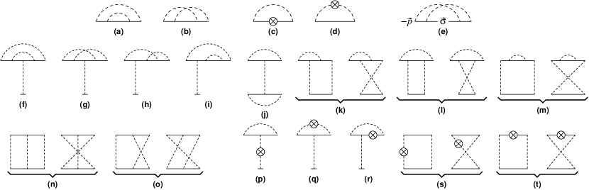
Figure 10: Two-loop diagrams for the self energy (a–e) and vertex (f–t) corrections.

Table 1: Two-loop diagrams. The first column contains combinatorial factors and diagram labels according to Fig. 10. The integrals relevant for the calculation of a given diagram are listed in the second column. The third column contains the divergent part of the diagram.

diagram	integrals used	result
self energy [in units $4\pi^{2}im\alpha_{0}^{2}c_{\varepsilon}^{2}/\varepsilon^{2}$]
(a)	(148)$\cdot$(149), (148)$\cdot$(150)	$-4+4\varepsilon$
(b)	(159), (160)	$-2$
self energy with counterterms [in units $4\pi^{2}im\alpha_{0}^{2}c_{\varepsilon}/4\pi\varepsilon^{2}$]
(c)	(149)	$4-4\varepsilon$
(d)	(148)	$8$
velocity
(e)	(161), (162)	$-4\pi^{2}\bm{\sigma}\mathbf{p}\,\alpha_{0}^{2}c_{\varepsilon}^{2}/\varepsilon$
vertex [in units $8\pi^{3}\alpha_{0}^{3}\mu^{\varepsilon}c_{\varepsilon}^{2}/\varepsilon^{2}$]
2$\times$(f)	(149)2, (149)$\cdot$(150)	$8-8\varepsilon-\langle 8\varepsilon\rangle$
2$\times$(g)	(161), (163)	$-4+4\varepsilon+\langle 4\varepsilon\rangle$
4$\times$(h)	(161), (163)	$8-8\varepsilon-\langle 8\varepsilon\rangle$
4$\times$(i)	(148)$\cdot$(157), (148)$\cdot$(158)	$-\langle 8\varepsilon\rangle$
(j)	(149)2, (149)$\cdot$(150)	$4-4\varepsilon-\langle 4\varepsilon\rangle$
4$\times$(k)	(163)	$-\langle 16\varepsilon\rangle$
2$\times$(l)	(163)	$0$
2$\times$(m)	(148)$\cdot$(157), (148)$\cdot$(158)	$0$
(n)	(149)2	$4-2\varepsilon$
2$\times$(o)	(161)	$-4+4\varepsilon$
vertex with counterterms [in units $8\pi^{3}\alpha_{0}^{3}\mu^{\varepsilon}c_{\varepsilon}/4\pi\varepsilon^{2}$]
2$\times$(p)	(149)	$-16+8\varepsilon+\langle 8\varepsilon\rangle$
2$\times$(q)	(149)	$-16+8\varepsilon+\langle 8\varepsilon\rangle$
4$\times$(r)	(157), (158)	$\langle 8\varepsilon\rangle$
2$\times$(s)	(150)	$\langle 16\varepsilon\rangle$
2$\times$(t)	(157), (158)	$0$

Let us calculate corrections to the self energy in two-loop order (including diagrams with the one-loop counterterms). The relevant diagrams are shown in Fig. 10a – 10e. The divergent parts of these diagrams and the integrals used in their calculation are given in Table 1. The divergent part of the self-energy correction is

$$\Sigma^{(2)}\big{|}_{p=0}=\frac{3i}{2}\,\frac{m\alpha_{0}^{2}}{\varepsilon^{2}}.$$ (164)

The divergence in $\Sigma^{(2)}$ is compensated by the second-order mass counterterm

$$\delta^{(2)}m=\frac{3}{2}\,\frac{m\alpha_{0}^{2}}{\varepsilon^{2}}.$$ (165)

Electron velocity $v_{0}$ also acquires a correction in two-loop order. This correction appears because the second-order self energy depends on the external momentum. Expanding $\Sigma^{(2)}$ in small external momentum we obtain the diagram Fig. 10e. It equals to

$$\text{(e)}=\mathbf{p}\,\frac{\partial\Sigma^{(2)}(\mathbf{p})}{\partial\mathbf{p}}\bigg{|}_{p=0}=\bm{\sigma}\mathbf{p}\,4\pi^{2}\alpha_{0}^{2}c_{\varepsilon}^{2}\biggl{[}-\frac{1}{\varepsilon}+\mathcal{O}(1)\biggr{]}.$$ (166)

This divergence is compensated by the velocity counterterm

$$\delta^{(2)}v_{0}=\frac{\alpha_{0}^{2}}{4\varepsilon}.$$ (167)

B.3.2 Vertex

The two-loop vertex diagrams are shown in Fig. 10f – 10t. The values of these diagrams are given in the bottom part of Table 1 along with the integrals used in their calculation. According to Refs. Bondi, ; Kivel, , one can disregard the mass in the numerator of the electron propagator (143). In order to check this fact, we keep the corresponding parts in angular brackets in Table 1. Indeed, these contributions sum up to zero.

The divergent part of the two-loop vertex correction is

$$\Gamma^{(2)}\big{|}_{p=0}=8\pi^{3}\alpha_{0}^{3}\mu^{\varepsilon}\left(\frac{16c_{\varepsilon}^{2}}{\varepsilon^{2}}-\frac{32c_{\varepsilon}}{4\pi\varepsilon^{2}}+\frac{2c_{\varepsilon}^{2}}{\varepsilon}\right)\\ =\pi\mu^{\varepsilon}\alpha_{0}^{3}\left(-\frac{8}{\varepsilon^{2}}+\frac{1}{\varepsilon}\right).$$ (168)

This divergence is canceled by the two-loop vertex counterterm

$$\delta^{(2)}\alpha_{0}=\alpha_{0}^{3}\left(\frac{4}{\varepsilon^{2}}-\frac{1}{2\varepsilon}\right).$$ (169)

B.4 RG equations

Now we collect the one and two-loop counterterms and compose the bare action of the model:

$$S_{B}=\!\int\!d^{2-\varepsilon}x\big{[}\bar{\psi}_{B}\bm{\sigma}\nabla\psi_{B}+m_{B}\bar{\psi}_{B}\psi_{B}+\pi\alpha_{0B}(\bar{\psi}_{B}\psi_{B})^{2}\big{]}\\ =\!\int\!d^{2-\varepsilon}x\bigg{[}\left(1+\frac{\alpha_{0}^{2}}{4\varepsilon}\right)\bar{\psi}\bm{\sigma}\nabla\psi+m\left(1-\frac{\alpha_{0}}{\varepsilon}+\frac{3\alpha_{0}^{2}}{2\varepsilon^{2}}\right)\bar{\psi}\psi\\ +\pi\alpha_{0}\mu^{\varepsilon}\left(1-\frac{2\alpha_{0}}{\varepsilon}+\frac{4\alpha_{0}^{2}}{\varepsilon^{2}}-\frac{\alpha_{0}^{2}}{2\varepsilon}\right)(\bar{\psi}\psi)^{2}\bigg{]}.$$ (170)

Parameters of this action are

$$\psi_{B} =\psi\left(1+\frac{\alpha_{0}^{2}}{8\varepsilon}\right),$$ (171)

$$m_{B} =m\left(1-\frac{\alpha_{0}}{\varepsilon}+\frac{3\alpha_{0}^{2}}{2\varepsilon^{2}}-\frac{\alpha_{0}^{2}}{4\varepsilon}\right),$$ (172)

$$\alpha_{0B} =\alpha_{0}\mu^{\varepsilon}\left(1-\frac{2\alpha_{0}}{\varepsilon}+\frac{4\alpha_{0}^{2}}{\varepsilon^{2}}-\frac{\alpha_{0}^{2}}{\varepsilon}\right).$$ (173)

By construction, the bare couplings $m_{B}$ and $\alpha_{0B}$ do not depend on the scale $\mu$,

$$\frac{\partial\alpha_{0B}}{\partial\ln\mu}=0,\qquad\frac{\partial m_{B}}{\partial\ln\mu}=0.$$ (174)

This determines scaling behavior of renormalized (observable) couplings:

$$\frac{\partial\alpha_{0}}{\partial\ln\mu} =-\varepsilon\alpha_{0}-2\alpha_{0}^{2}-2\alpha_{0}^{3},$$ (175)

$$\frac{\partial m}{\partial\ln\mu} =-m\alpha_{0}-\frac{m\alpha_{0}^{2}}{2}.$$ (176)

We express the result in the form of real-space scaling with $\Lambda\sim\mu^{-1}$. This amounts to changing the sign of the derivatives. Taking the limit $\varepsilon\to 0$ and replacing mass by the energy ($m=-i\epsilon$), we finally obtain the RG equations in the form

$$\frac{\partial\alpha_{0}}{\partial\ln\Lambda} =2\alpha_{0}^{2}+2\alpha_{0}^{3},$$ (177)

$$\frac{\partial\epsilon}{\partial\ln\Lambda} =\epsilon\left(\alpha_{0}+\frac{\alpha_{0}^{2}}{2}\right).$$ (178)

As discussed above [see Eqs. (138) – (140)], the second-loop term in the RG equation for energy (178) is not universal. This is easily demonstrated with the help of a small redefinition of $\alpha_{0}$,

$$\alpha_{0}^{\prime} =\alpha_{0}+M\alpha_{0}^{2},$$ (179)

$$\frac{\partial\epsilon}{\partial\ln\Lambda} =\epsilon\left(\alpha_{0}^{\prime}+\frac{{\alpha_{0}^{\prime}}^{2}}{2}-M{\alpha_{0}^{\prime}}^{2}\right).$$ (180)

On the contrary, the two-loop term in the beta function for $\alpha_{0}$ remains unchanged as the RG equation (177), being dimensionless, cannot contain $\epsilon$. In the main text, we use only universal one-loop part of the energy beta function.

Appendix C Analysis of one-loop RG equations

In this Appendix we will analyze the set of coupled RG equations (77), (78) and (79) assuming that all three couplings are nonzero. It is convenient to introduce new couplings

$$\alpha_{1} = \alpha_{\perp}+\alpha_{z}~{},$$ (181)

$$\alpha_{2} = \alpha_{\perp}-2\alpha_{z}~{}.$$ (182)

In terms of these couplings the one-loop RG equations take the form

$$\frac{\partial\alpha_{0}}{\partial\ln\Lambda} =2\alpha_{0}^{2}+2\alpha_{0}\alpha_{1}+\frac{2}{9}(2\alpha_{1}+\alpha_{2})(\alpha_{1}-\alpha_{2}),$$ (183)

$$\frac{\partial\alpha_{1}}{\partial\ln\Lambda} =2\alpha_{0}\alpha_{1}+\frac{2}{9}(\alpha_{1}+2\alpha_{2})(\alpha_{1}-\alpha_{2}),$$ (184)

$$\frac{\partial\alpha_{2}}{\partial\ln\Lambda} =-4\alpha_{0}\alpha_{2}-\frac{4}{9}(\alpha_{1}+2\alpha_{2})(\alpha_{1}-\alpha_{2}).$$ (185)

It follows that the couplings $\alpha_{0}$ and $\alpha_{1}$ grow upon the renormalization. Furthermore, comparing Eqs. (183) and (184), one sees that the coupling $\alpha_{0}$ increases faster than $\alpha_{1}$. On the other hand, the coupling $\alpha_{2}$ decreases, which allows us to neglect $\alpha_{2}$ in Eqs. (183) and (184) as the first approximation:

$$\frac{\partial\alpha_{0}}{\partial\ln\Lambda} =2\alpha_{0}^{2}+2\alpha_{0}\alpha_{1}+\frac{4}{9}\alpha_{1}^{2},$$ (186)

$$\frac{\partial\alpha_{1}}{\partial\ln\Lambda} =2\alpha_{0}\alpha_{1}+\frac{2}{9}\alpha_{1}^{2}.$$ (187)

Let us consider the ratio of the couplings, which we denote

$$g_{1}=\frac{\alpha_{1}}{\alpha_{0}}.$$ (188)

Using Eqs. (186) and (187), we obtain the RG equation for $g_{1}$ in the form

$$\frac{\partial g_{1}}{\partial\ln\Lambda}=-\frac{16}{9}\;g_{1}^{2}\left(\alpha_{0}+\frac{1}{4}\alpha_{1}\right).$$ (189)

Assume bare values of the three couplings are of the same order, $\alpha_{0}\sim\alpha_{\perp}\sim\alpha_{z}\sim\alpha$. Since $\alpha_{0}$ grows faster than $\alpha_{1}$, for the “first iteration” we retain only $\alpha_{0}$ in Eq. (189). We find

$$\frac{1}{g_{1}(\Lambda)}\simeq\frac{1}{g_{1}}+\frac{16}{9}\int_{a}^{\Lambda}\frac{d\tilde{\Lambda}}{\tilde{\Lambda}}\;\alpha_{0}(\tilde{\Lambda}).$$ (190)

Further, neglecting $\alpha_{1}$ also in Eq. (186), dividing this equation by $\alpha_{0}$, and integrating the result over $d\ln\Lambda$, we find

$$2\int_{a}^{\Lambda}\frac{d\tilde{\Lambda}}{\tilde{\Lambda}}\;\alpha_{0}(\tilde{\Lambda})=\ln\frac{\alpha_{0}(\Lambda)}{\alpha}.$$ (191)

When $\alpha_{0}$ reaches unity (this happens when $\epsilon<\gamma$), combining Eqs. (190) and (191), we have

$$\frac{1}{g_{1}(\Lambda)}=\frac{1}{\alpha_{1}}\simeq\frac{1}{g_{1}}+\frac{8}{9}\ln\frac{1}{\alpha}.$$ (192)

We arrive at the conclusion that at the end of the renormalization the scalar potential becomes the dominating disorder:

$$\left.\frac{\alpha_{0}}{\alpha_{\perp}+\alpha_{z}}\right|_{\alpha_{0}\simeq 1}\simeq\frac{8}{9}\ln\frac{1}{\alpha}\gg 1.$$ (193)

This result can be refined by retaining $\alpha_{1}$ in Eqs. (186), (187), and (189), which yields a correction $\simeq-(3/4)\ln|\ln\alpha|$ to Eq. (193).

Above we assumed that all three couplings are of the same order at the ultraviolet scale. The generalization onto the case of non-equal couplings is straightforward. It turns out that in the ultraballistic regime (when the renormalization stops by the largest coupling reaching unity) the scalar potential always wins, whatever the initial couplings are.

References

- (1) K.S. Novoselov, A.K. Geim, S.V. Morozov, D. Jiang, Y. Zhang, S.V. Dubonos, I.V. Grigorieva, and A.A. Firsov, Science 306, 666 (2004).
- (2) K.S. Novoselov, D. Jiang, F. Schedin, T.J. Booth, V.V. Khotkevich, S.V. Morozov, and A.K. Geim, Proc. Natl. Acad. Sci. U.S.A. 102, 10451 (2005).
- (3) K.S. Novoselov, A.K. Geim, S.V. Morozov, D. Jiang, M.I. Katsnelson, I.V. Grigorieva, S.V. Dubonos, and A.A. Firsov, Nature (London) 438, 197 (2005).
- (4) Y. Zhang, Y.-W. Tan, H.L. Stormer, and P. Kim, Nature (London) 438, 201 (2005).
- (5) Y.-W. Tan, Y. Zhang, H.L. Stormer, and P. Kim, Eur. Phys. J. Special Topics, 148, 15 (2007).
- (6) A.K. Geim and K.S. Novoselov, Nature Materials 6, 183 (2007).
- (7) A.H. Castro Neto, F. Guinea, N.M.R. Peres, K.S. Novoselov, and A.K. Geim, arXiv:0709.1163, to appear in Rev. Mod. Phys.
- (8) I.L. Aleiner and K.B. Efetov, Phys. Rev. Lett. 97, 236801 (2006).
- (9) A. Altland, Phys. Rev. Lett. 97, 236802 (2006).
- (10) P.M. Ostrovsky, I.V. Gornyi, and A.D. Mirlin, Phys. Rev. B 74, 235443 (2006).
- (11) P.M. Ostrovsky, I.V. Gornyi, and A.D. Mirlin, Phys. Rev. Lett. 98, 256801 (2007).
- (12) P.M. Ostrovsky, I.V. Gornyi, and A.D. Mirlin, Eur. Phys. J. Special Topics 148, 63 (2007).
- (13) P.M. Ostrovsky, I.V. Gornyi, and A.D. Mirlin, Phys. Rev. B 77, 195430 (2008).
- (14) E. McCann, K. Kechedzhi, V.I. Fal’ko, H. Suzuura, T. Ando, and B.L. Altshuler, Phys. Rev. Lett. 97, 146805 (2006).
- (15) A.F. Morpurgo and F. Guinea, Phys. Rev. Lett. 97, 196804 (2006).
- (16) S. Ryu, C. Mudry, H. Obuse, and A. Furusaki, Phys. Rev. Lett. 99, 116601 (2007).
- (17) K. Nomura, M. Koshino, and S. Ryu, Phys. Rev. Lett. 99, 146806 (2007).
- (18) D. Hsieh, D. Qian, L. Wray, Y. Xia, Y. Hor, R.J. Cava and M.Z. Hasan Nature 452, 970 (2008).
- (19) A.P. Schnyder, S. Ryu, A. Furusaki, and A.W.W. Ludwig, arXiv:0803.2786
- (20) K. Nomura and A.H. MacDonald, Phys. Rev. Lett. 98, 076602 (2007).
- (21) A. Rycerz, J. Tworzydlo, and C.W.J. Beenakker, Europhys.Lett. 79, 57003 (2007).
- (22) J.H. Bardarson, J. Tworzydło, P.W. Brouwer, and C.W.J. Beenakker, Phys. Rev. Lett. 99, 106801 (2007).
- (23) P. San-Jose, E. Prada, and D.S. Golubev, Phys. Rev. B 76, 195445 (2007).
- (24) C.H. Lewenkopf, E.R. Mucciolo, and A.H. Castro Neto, Phys. Rev. B 77, 081410R (2008).
- (25) M.I. Katsnelson, Eur. Phys. J. B 51, 157 (2006).
- (26) J. Tworzydlo, B. Trauzettel, M. Titov, A. Rycerz, and C.W.J. Beenakker, Phys. Rev. Lett. 96, 246802 (2006).
- (27) H.B. Heersche, P. Jarillo-Herrero, J.B. Oostinga, L.M.K. Vandersypen, and A.F. Morpurgo, Nature 446, 56 (2007).
- (28) F. Miao, S. Wijeratne, Y. Zhang, U.C. Coskun, W. Bao, and C.N. Lau, Science 317, 1530 (2007).
- (29) R. Danneau, F. Wu, M.F. Craciun, S. Russo, M.Y. Tomi, J. Salmilehto, A.F. Morpurgo, and P.J. Hakonen, Phys. Rev. Lett. 100, 196802 (2008).
- (30) R. Danneau, F. Wu, M.F. Craciun, S. Russo, M.Y. Tomi, J. Salmilehto, A.F. Morpurgo, and P.J. Hakonen, arXiv:0807.0157.
- (31) C.W.J. Beenakker, Rev. Mod. Phys. 69, 731 (1997).
- (32) S. Ryu, C. Mudry, A. Furusaki, and A.W.W. Ludwig, Phys. Rev. B 75, 205344 (2007).
- (33) Some analytical results for ballistic transport in graphene were obtained within the toy-model of one-dimensional disorder in Refs. San-Jose07, ; Titov07, . In the present paper, we address the realistic case of a truly two-dimensional disorder.
- (34) M. Titov, Europhys. Lett. 79, 17004 (2007).
- (35) M. Titov and C.W.J. Beenakker, Phys. Rev. B 74, 041401(R) (2006).
- (36) V.V. Cheianov and V.I. Fal’ko, Phys. Rev. B 74, 041403 (2006).
- (37) F.V. Tikhonenko, D.W. Horsell, R.V. Gorbachev, and A.K. Savchenko, Phys. Rev. Lett. 100, 056802 (2008).
- (38) T. Ando, J. Phys. Soc. Jpn 75, 074716 (2006).
- (39) K. Nomura and A.H. MacDonald, Phys. Rev. Lett. 96, 256602 (2006).
- (40) D.V. Khveshchenko, Phys. Rev. B 75, 241406(R) (2007).
- (41) The linear dependence of the conductivity on the gate voltage (with logarithmic corrections) could also be explained within the model of very strong short-range scatterers (unitary limit), such as, e.g., vacancies or substitutional defects, see Ref. OurPRB, . However, this type of disorder is not observed by microscopy studies and would be in conflict OurQHE with the observed odd-integer quantum Hall effect.
- (42) At finite Fermi energy in the contacts, the right- and left-moving components of get mixed outside the sample. However, this effect disappears in the limit .
- (43) O.N. Dorokhov, Zh. Eksp. Teor. Fiz. 85, 1040 (1983) [Sov. Phys. JETP 58, 606 (1983)].
- (44) H. Lee, L.S. Levitov, and A.Yu. Yakovets, Phys. Rev. B 51 4079 (1995).
-
(45)
To avoid confusion, we adopt the following convention for elliptic integrals:
One often uses an alternative notation, and , with the modulus as an argument. - (46) H. Schomerus, Phys. Rev. B 76, 045433 (2007).
- (47) Ya.M. Blanter and I. Martin, Phys. Rev. B 76, 155433 (2007).
- (48) V.S. Dotsenko and V.S. Dotsenko, Adv. Phys. 32, 129 (1983).
- (49) A.W.W. Ludwig, M.P.A. Fisher, R. Shankar, and G. Grinstein, Phys. Rev. B 50, 7526 (1994);
- (50) A.M. Tsvelik, Phys. Rev. B 51, 9449 (1995).
- (51) A. A. Nersesyan, A. M. Tsvelik, and F. Wenger, Phys. Rev. Lett. 72, 2628 (1994); Nucl. Phys. B 438, 561 (1995).
- (52) M. Bocquet, D. Serban, and M.R. Zirnbauer, Nucl. Phys. B 578,628 (2000).
- (53) A. Altland, B.D. Simons, and M.R. Zirnbauer, Phys. Rep. 359, 283 (2002).
- (54) S. Guruswamy, A. LeClair, and A.W.W. Ludwig, Nucl. Phys. B 583, 475 (2000).
- (55) In Ref. OurPRB , the beta function for energy contains an extra term corresponding to the normal dimension of . In the present work we adopt an alternative approach with the running band width.
- (56) Yu.V. Nazarov, Phys. Rev. Lett. 73, 134 (1994).
- (57) Yu. Nazarov, Ann. Phys. (Leipzig) 8, 193 (1999).
- (58) D.B. Gutman, Y. Gefen, and A.D. Mirlin, in ”Quantum Noise in Mesoscopic Physics”, edited by Yu.V. Nazarov (Kluwer, 2003), pp.497-524.
- (59) D.B. Gutman, A.D. Mirlin, and Y. Gefen, Phys. Rev. B 71, 085118 (2005).
- (60) M.M. Fogler, F. Guinea, M.I. Katsnelson, arXiv:0807.3165.
- (61) M. Titov, private communication.
- (62) F. Evers and A.D. Mirlin, arXiv:0707.4378.
- (63) When or initially dominate and the energy is sufficiently high, RG stops before exceeds other couplings. At such energies antilocalization regime does not occur.
- (64) J. Gonzalez, F. Guinea, and M.A.H. Vozmediano, Nucl. Phys. B 424, 596 (1994).
- (65) M.S. Foster and I.L. Aleiner, Phys. Rev. B 77, 195413 (2008).
- (66) M.S. Foster and A.W.W. Ludwig, Phys. Rev. B 73, 155104 (2006).
- (67) M.E. Peskin and D.V. Schroeder, An Introduction to Quantum Field Theory, Addison-Wesley Advanced Book Program (Westview Press, Boulder, 1995).
- (68) A. Bondi, G. Curci, G. Pattuti, and P. Rossi, Ann. Phys. 199, 268 (1990).
- (69) A.N. Vasil’ev, M.I. Vyazovskii, S.E. Derkachev, and N.A. Kivel’, Theor. Math. Phys. 107, 441 (1996).