Abstract

This paper is concerned with the stability problem for the planar linear switched system $\dot{x}(t)=u(t)A_{1}x(t)+(1-u(t))A_{2}x(t)$, where the real matrices $A_{1},A_{2}\in{R}^{2\times 2}$ are Hurwitz and $u(\cdot):[0,\infty[\to\{0,1\}$ is a measurable function. We give coordinate-invariant necessary and sufficient conditions on $A_{1}$ and $A_{2}$ under which the system is asymptotically stable for arbitrary switching functions $u(\cdot)$. The new conditions unify those given in previous papers and are simpler to be verified since we are reduced to study 4 cases instead of 20. Most of the cases are analyzed in terms of the function $\Gamma(A_{1},A_{2})=\frac{1}{2}({\rm tr}(A_{1}){\rm tr}(A_{2})-{\rm tr}(A_{1}A_{2}))$.

Keywords: planar switched systems, asymptotic stability, quadratic Lyapunov functions

1 Introduction

Let $A_{1}$ and $A_{2}$ be two $2\times 2$ real Hurwitz matrices. In this paper we are concerned with the problem of finding necessary and sufficient conditions on $A_{1}$ and $A_{2}$ under which the switched system

$$\dot{x}(t)=u(t)A_{1}x(t)+(1-u(t))A_{2}x(t),\leavevmode\nobreak\ \leavevmode\nobreak\ x=(x_{1},x_{2})\in{R}^{2},{}$$ (1)

is globally asymptotically stable, uniformly with respect to measurable switching functions $u(\cdot):[0,\infty[\to\{0,1\}$ (GUAS for short, see Definition 1 below).

This problem has been studied in [3] in the case in which both $A_{1}$ and $A_{2}$ are diagonalizable in ${C}$ (diagonalizable case in the following) and in [1] in the case in which at least one among $A_{1}$ and $A_{2}$ is not (nondiagonalizable case in the following). (See also [7] as well as the related work [6].)

In both cases the stability conditions are given in terms of coordinate-invariant parameters. Unfortunately the parameters used in the diagonalizable case become singular in the nondiagonalizable one and therefore the two cases were studied separately.

The purpose of this note is to unify and simplify these conditions, reformulating them in terms of new invariants that permit to treat all cases at the same time.

We have reduced the cases to be studied from 20 (14 in the diagonalizable case and 6 in the nondiagonalizable one) to the following 4 cases (see Theorem 1).

S1:

the first one corresponds to the case in which there exists a common quadratic Lyapunov function. The condition of S1 is indeed equivalent to the condition given in [10] but is simpler to check. Recall however that the existence of a common quadratic Lyapunov function is only a sufficient condition for GUAS (i.e. there exist GUAS systems not admitting a quadratic Lyapunov function). See [4, 7] for details.

S2:

the second one corresponds to the situation in which there exists $v\in(0,1)$ such that $vA_{1}+(1-v)A_{2}$ has a positive real eigenvalue. In this case the system is unbounded since it is possible to build a trajectory going to infinity approximating the (non admissible) trajectory corresponding to $u(t)\equiv v$ and having the direction of the unstable eigenvector of $vA_{1}+(1-v)A_{2}$.

S3:

in the third case there exists a nonstrict common quadratic Lyapunov function. The system is only uniformly stable, but not GUAS, since there exists a trajectory not tending to the origin when $t$ goes to infinity.

S4:

in the fourth case the stability analysis of the system reduces to the study of a single trajectory called worst trajectory. If this trajectory tends to the origin then the system is GUAS (in this case there exists a polynomial Lyapunov function, but not a quadratic one). If it is periodic then the system is uniformly stable but not GUAS. If it is unbounded then the system is unbounded.

For a discussion of various issues related to stability of switched systems, we refer the reader to [4, 5].

The paper is organized as follows. In Section 1.1 we recall the fundamental notions of stability and the different types of Lyapunov functions used in the paper. Section 2 contains our main result. In Section 3.1 we define the normal forms that are needed in the proof. In Section 3.2 we give the details of the proof.

1.1 Notions of stability

Let us recall some classical notions of stability which will be used in the following.

Definition 1

For $\delta>0$ let $B_{\delta}$ be the unit ball of radius $\delta$, centered in the origin. Denote by ${\mathcal{U}}$ the set of measurable functions defined on $[0,\infty[$ and taking values on $\{0,1\}$. Given $x_{0}\in{R}^{2}$, we denote by $\gamma_{x_{0},u(\cdot)}(\cdot)$ the trajectory of (1) based in $x_{0}$ and corresponding to the control $u(\cdot)$. We say that the system (1) is

• unbounded at the origin if there exist $x_{0}\in{R}^{2}$ and $u(\cdot)\in{\mathcal{U}}$ such that $\gamma_{x_{0},u(\cdot)}(t)$ goes to infinity as $t$ goes to infinity;

• uniformly stable at the origin if for every $\varepsilon>0$ there exists $\delta>0$ such that $\gamma_{x_{0},u(\cdot)}(t)\in B_{\varepsilon}$ for every $t>0$, for every $u(\cdot)\in{\mathcal{U}}$ and every $x_{0}\in B_{\delta}$;

• globally uniformly asymptotically stable at the origin (GUAS, for short) if it is uniformly stable at the origin and globally uniformly attractive, i.e., for every $\delta_{1},\delta_{2}>0$, there exists $T>0$ such that $\gamma_{x_{0},u(\cdot)}(t)\in B_{\delta_{1}}$ for every $t\geq T$, for every $u(\cdot)\in{\mathcal{U}}$ and every $x_{0}\in B_{\delta_{2}}$.

Remark 1

The stability properties of the system (1) do not change if we allow measurable switching functions taking values in $[0,1]$ instead of $\{0,1\}$ (see for instance [7]). More precisely the system (1) with $u(\cdot):[0,\infty[\to\{0,1\}$ is GUAS (resp. uniformly stable, resp. unbounded) if and only the system (1) with $u(\cdot):[0,\infty[\to[0,1]$ is. In the following we name convexified system the switched system with $u(\cdot)$ taking values in $[0,1]$.

Since the stability properties of the system (1) do not depend on the parametrization of the integral curves of $A_{1}x$ and $A_{2}x$, we have the following.

Lemma 1

If the switched system $\dot{x}=u(t)A_{1}x+(1-u(t))A_{2}x,\leavevmode\nobreak\ \leavevmode\nobreak\ \leavevmode\nobreak\ u(\cdot):[0,\infty[\to\{0,1\},$ has one of the stability properties given in Definition 1, then the same stability property holds for the system $\dot{x}=u(t)(A_{1}/\alpha_{1})x+(1-u(t))(A_{2}/\alpha_{2})x$, for every $\alpha_{1},\alpha_{2}>0$.

Definition 2

A common Lyapunov function ( LF for short) $V:{R}^{2}\longrightarrow{R}^{+}$ for a switched system of the form (1) is a continuous function such that $V(\cdot)$ is positive definite (i.e. $V(x)>0$, $\forall x\neq 0$, $V(0)=0$) and $V(\cdot)$ is strictly decreasing along nonconstant trajectories.

A positive definite continuous function $V:{R}^{2}\longrightarrow{R}^{+}$ is said to be a nonstrict common Lyapunov function if $V(\cdot)$ is nonincreasing along nonconstant trajectories.

A common quadratic Lyapunov function (quadratic LF for short) is a function of the form $V(x)=x^{T}Px$ where $P$ is a positive definite symmetric matrix and the matrices $A_{1}^{T}P+PA_{1}$ and $A_{2}^{T}P+PA_{2}$ are negative definite.

We recall that, for systems of type (1), the existence of a LF  is equivalent to GUAS (see for instance [4]). Moreover the existence of a nonstrict LF guarantees the uniform stability of (1).

2 Stability conditions for two-dimensional bilinear switched systems

We start this section by defining the notations and the objects that will be used to state our stability result. In the following the word invariant will indicate any object which is invariant with respect to coordinate transformations. As usual, we denote by $\det(X)$ and ${\rm tr}(X)$ the determinant and the trace of a matrix $X$. If $X\in{R}^{2\times 2}$ the discriminant is defined as

$$\delta_{X}={\rm tr}(X)^{2}-4\,\det(X)\,.$$

Given a pair of matrices $X,Y$ we define the following object:

$$\Gamma(X,Y):=\displaystyle\frac{1}{2}({\rm tr}(X){\rm tr}(Y)-{\rm tr}(XY))\,.$$

By means of these invariants we can define the following invariants associated to (1):

$$\tau_{i}:=\left\{\begin{array}[]{l}\displaystyle\frac{{\rm tr}(A_{i})}{\sqrt{|\delta_{A_{i}}|}}\quad\mbox{ if }\ \delta_{A_{1}}\neq 0\,,\ \delta_{A_{2}}\neq 0\,,\\ \displaystyle\frac{{\rm tr}(A_{i})}{\sqrt{|\delta_{A_{j}}|}}\quad\mbox{ if }\ \delta_{A_{1}}\delta_{A_{2}}=0\mbox{ but }\delta_{A_{j}}\neq 0\,,\\ \displaystyle\frac{{\rm tr}(A_{i})}{2}\quad\mbox{ if }\ \delta_{A_{1}}=\delta_{A_{2}}=0\,,\end{array}\right.$$ (5)

$$k:=\displaystyle\frac{2\tau_{1}\tau_{2}}{{\rm tr}(A_{1}){\rm tr}(A_{2})}\Big{(}{\rm tr}(A_{1}A_{2})-\frac{1}{2}{\rm tr}(A_{1}){\rm tr}(A_{2})\Big{)}\,,$$

$$\Delta:=4(\Gamma(A_{1},A_{2})^{2}-\Gamma(A_{1},A_{1})\Gamma(A_{2},A_{2}))\,.$$

$$\mathcal{R}:=\displaystyle\frac{2\Gamma(A_{1},A_{2})+\sqrt{\Delta}}{2\sqrt{\det(A_{1})\det(A_{2})}}e^{\tau_{1}t_{1}+\tau_{2}t_{2}}\,,\mbox{where, for }\ i=1,2\,,$$

$$t_{i}:=\left\{\begin{array}[]{lr}\frac{\pi}{2}-\mbox{arctan}\frac{{\rm tr}(A_{1}){\rm tr}(A_{2})(k\tau_{i}+\tau_{3-i})}{2\tau_{1}\tau_{2}\sqrt{\Delta}}&\mbox{ if }\ \delta_{A_{i}}<0\\ \mbox{arctanh}\frac{2\tau_{1}\tau_{2}\sqrt{\Delta}}{{\rm tr}(A_{1}){\rm tr}(A_{2})(k\tau_{i}-\tau_{3-i})}&\mbox{ if }\ \delta_{A_{i}}>0\\ \frac{2\sqrt{\Delta}}{({\rm tr}(A_{1}A_{2})-{\rm tr}(A_{1}){\rm tr}(A_{2})/2)\tau_{i}}&\mbox{if }\ \delta_{A_{i}}=0\end{array}\right.\,.$$ (9)

Remark 2

Let us define

$$sign(x):=\left\{\begin{array}[]{r}+1\ \mbox{ if $x>0$ }\\ 0\ \mbox{ if $x=0$ }\\ -1\ \mbox{ if $x<0$ }\end{array}\right.\,.$$

Notice that, for every matrix $X\in{R}^{2\times 2}$, one has $\Gamma(X,X)=\det(X)$. Also, since the Killing form of ${R}^{2\times 2}$ is defined as $\mathcal{B}(X,Y)=4\,{\rm tr}(XY)-2\,{\rm tr}(X){\rm tr}(Y)$ one has $sign(k)=sign(\mathcal{B}(A_{1},A_{2}))$. Finally, notice that if $A_{1},A_{2}$ are Hurwitz then $\tau_{i}<0\,$ for $\,i=1,2\,$ and $\ sign\,\Gamma(A_{1},A_{2})=sign(\tau_{1}\tau_{2}-k)$.

2.1 Statement of the results

In this section we state our main result which characterizes conpletely the stability properties of two-dimensional bilinear switched systems. Our necessary and sufficient conditions apply both to the non-degenarate cases studied in [3] and to the degenarate ones studied in [1].

Theorem 1

We have the following stability conditions for the system (1)

S1

If   $\Gamma{(A_{1},A_{2})}>-\sqrt{\det(A_{1})\det(A_{2})},\ \text{and}\ {\rm tr}(A_{1}A_{2})>-2\sqrt{\det(A_{1})\det(A_{2})}$ then the system admits a quadratic LF.

If   $-\sqrt{\det(A_{1})\det(A_{2})}<\Gamma(A_{1},A_{2})\leq\sqrt{\det(A_{1})\det(A_{2})}$ then the condition ${\rm tr}(A_{1}A_{2})>-2\sqrt{\det(A_{1})\det(A_{2})}$ is automatically satisfied. As a consequence the system admits a quadratic LF.

S2

If  $\Gamma{(A_{1},A_{2})}<-\sqrt{\det(A_{1})\det(A_{2})},$ then the system is unbounded,

S3

If  $\Gamma{(A_{1},A_{2})}=-\sqrt{\det(A_{1})\det(A_{2})},$ then the system is uniformly stable but not GUAS,

S4

If   $\Gamma{(A_{1},A_{2})}>\sqrt{\det(A_{1})\det(A_{2})},\ \ \text{and}\ \ {\rm tr}(A_{1}A_{2})\leq-2\sqrt{\det(A_{1})\det(A_{2})}$ then the system is GUAS, uniformly stable (but not GUAS) or unbounded respectively if

$${\mathcal{R}}<1,{\mathcal{R}}=1,{\mathcal{R}}>1.$$

The following corollary will be derived from item S1 of the previous theorem.

Corollary 1

If $\det([A_{1},A_{2}])\geq 0$ then the system admits a quadratic LF.

Remark 3

In the diagonalizable case $\delta_{A_{1}}\delta_{A_{2}}\neq 0$ the parameters $\tau_{1}$, $\tau_{2}$, and $k$ are invariant under the transformation $(A_{1},A_{2})\to(A_{1}/\alpha_{1},A_{2}/\alpha_{2})$, for every $\alpha_{1},\alpha_{2}>0.$ This is no more true in the nondiagonalizable case. Notice however that in any case the stability conditions of Theorem 1 do not depend on coordinate transformations or on rescalings of the type $(A_{1},A_{2})\to(A_{1}/\alpha_{1},A_{2}/\alpha_{2})$. This is true in particular for the function $\mathcal{R}$.

3 Proof of the main results

3.1 Normal forms

The aim of this section is to reduce all the possible choices of the matrices $A_{1},A_{2}$ to suitable normal forms, obtained up to coordinates transformations and rescaling of the matrices (see Lemma 1 and Remark 3 above), and depending directly on the coordinate invariant parameters introduced above. The normal forms used here describe all the possible situations for two-dimensional bilinear switched systems, covering at the same time the diagonalizable case studied in [3] and the nondiagonalizable one studied in [1]. They will play a key role in the proof of our results.

Lemma 2

We have the following cases depending on the rank of $[A_{1},A_{2}]$:

1. If $\det([A_{1},A_{2}])\neq 0$, up to a linear change of coordinates and a renormalization according to Lemma 1, we can assume the following.

   $$A_{1}=\left(\begin{array}[]{cc}\tau_{1}&1\\ sign(\delta_{A_{1}})&\tau_{1}\end{array}\right),$$ (12)

   1. If $\det([A_{1},A_{2}])<0$ there exists $F\in\mathbb{R}$, $|F|\geq 1$ such that

      $$F+\frac{sign(\delta_{A_{1}}\delta_{A_{2}})}{F}=2k$$

      and $A_{2}$ has the form

      $$A_{2}=\left(\begin{array}[]{cc}\tau_{2}&sign(\delta_{A_{2}})/F\\ F&\tau_{2}\end{array}\right).$$ (15)

   2. If $\det([A_{1},A_{2}])>0$ then $\delta_{A_{i}}>0$ for $i=1,2$, $k\in(-1,1)$ and $A_{2}$ has the form

      $$A_{2}=\left(\begin{array}[]{cc}\tau_{2}+\sqrt{1-k{{}^{2}}}&k\\ k&\tau_{2}-\sqrt{1-k{{}^{2}}}\end{array}\right).$$ (18)

2. Under the hypothesis that $rank([A_{1},A_{2}])=1$, it is always possible, up to exchanging $A_{1}$ and $A_{2}$, to find a linear change of coordinates which diagonalizes $A_{1}$ and renders $A_{2}$ upper triangular.

3. If $[A_{1},A_{2}]=0$ then it must be $sign(\delta_{A_{1}})=sign(\delta_{A_{2}})$. If $\delta_{A_{i}}<0$ for $i=1,2$ or $\delta_{A_{i}}>0$ for $i=1,2$ then, up to a linear change of coordinates and a renormalization according to Lemma 1, $A_{1},A_{2}$ assume the form (12) and (15), respectively, with $F=k=\pm 1$. If $\delta_{A_{1}}=\delta_{A_{2}}=0$ then $A_{1},A_{2}$ can be put in upper triangular form with the elements of $A_{i}$ equal to $\tau_{i}$ on the diagonal, for $i=1,2$.

Proof of Lemma 2. For simplicity we will prove the lemma just in the case $\det([A_{1},A_{2}])\neq 0$, the other case being analogous. Note that Lemma 2 was proven in [3] when $\delta_{A_{1}}<0,\ \delta_{A_{2}}<0$ and in [1] in the case $\delta_{A_{1}}\delta_{A_{2}}=0$. Therefore, we can assume either $\delta_{A_{1}}>0$ or $\delta_{A_{2}}>0$. First consider the case $\delta_{A_{1}}>0$. In this case we can find a system of coordinates such that

$$A_{1}=\left(\begin{array}[]{cc}\lambda_{1}&0\\ 0&\lambda_{2}\end{array}\right),\leavevmode\nobreak\ \leavevmode\nobreak\ \leavevmode\nobreak\ A_{2}=\left(\begin{array}[]{cc}a&b\\ c&d\end{array}\right),\leavevmode\nobreak\ \leavevmode\nobreak\ a,b,c,d\in{R}.$$ (23)

Without any loss of generality we can assume that $\lambda_{1}<\lambda_{2}.$ The discriminant of $A_{1}$ is $(\lambda_{2}-\lambda_{1})^{2}$ and the discriminant of $A_{2}$ is $\delta_{A_{2}}=(a-d)^{2}+4bc$, which can be positive or negative. We have

$$[A_{1},A_{2}]=\left(\begin{array}[]{cc}0&{b(\lambda_{1}-\lambda_{2})}\\ c(\lambda_{2}-\lambda_{1})&0\end{array}\right).$$ (26)

Therefore $\det{[A_{1},A_{2}]}=bc(\lambda_{1}-\lambda_{2})^{2}\ \ \text{and}\ \ \delta_{[A_{1},A_{2}]}=-4bc(\lambda_{1}-\lambda_{2})^{2}$ and $k=\frac{d-a}{\sqrt{|\delta_{A_{2}}|}}$. If $\det{[A_{1},A_{2}]}<0$ consider the linear transformation

$$T=\left(\begin{array}[]{cc}-\sqrt{\frac{-b}{c}}&\sqrt{\frac{-b}{c}}\\ 1&1\end{array}\right)\,,$$

which diagonalizes $[A_{1},A_{2}]$. Then a straightforward computation shows that

$$\frac{2}{\sqrt{|\delta_{A_{1}}|}}T^{-1}A_{1}T=\left(\begin{array}[]{cc}\tau_{1}&1\\ 1&\tau_{1}\end{array}\right)\qquad\mbox{and}\qquad\frac{2}{\sqrt{|\delta_{A_{2}}|}}T^{-1}A_{2}T=\left(\begin{array}[]{cc}\tau_{2}&sign(\delta_{A_{2}})/F\\ F&\tau_{2}\end{array}\right),$$

where $F$ satisfies the equation $F+sign(\delta_{A_{2}})/F=2k$, and moreover we can assume $|F|\geq 1$ up to eventually exchange the reference coordinates. If $\delta_{A_{1}}<0$ then it must be $\delta_{A_{2}}>0$ and, exchanging the roles of $A_{1}$ and $A_{2}$, we can repeat the previous procedure obtaining

$$A_{1}=\left(\begin{array}[]{cc}\tau_{1}&sign(\delta_{A_{1}})/F\\ F&\tau_{1}\end{array}\right)\,,\leavevmode\nobreak\ \leavevmode\nobreak\ \leavevmode\nobreak\ \leavevmode\nobreak\ A_{2}=\left(\begin{array}[]{cc}\tau_{2}&1\\ sign(\delta_{A_{2}})&\tau_{2}\end{array}\right).$$

Then the required normal forms are obtained by exchanging the coordinates and by a dilation along one of the coordinate axis.

Consider now the case $\det{[A_{1},A_{2}]}=bc(\lambda_{1}-\lambda_{2})^{2}>0.$ We have

$$bc>0\leavevmode\nobreak\ \leavevmode\nobreak\ \Rightarrow\leavevmode\nobreak\ \leavevmode\nobreak\ \delta_{A_{2}}=(a-d)^{2}+4bc>0\ \ \text{and}\ \ |k|=\frac{|a-d|}{\sqrt{(a-d)^{2}+4bc}}<1\,.$$

In this case $[A_{1},A_{2}]$ is no more diagonalizable. Using the transformation

$$U=\left(\begin{array}[]{cc}\frac{1}{c}\sqrt{bc}&-\frac{1}{c}\sqrt{bc}\\ 1&1\end{array}\right)$$

we get

$$\frac{2}{\sqrt{|\delta_{A_{1}}|}}U^{-1}A_{1}U=\left(\begin{array}[]{cc}\tau_{1}&1\\ 1&\tau_{1}\end{array}\right)\qquad\mbox{and}\qquad\frac{2}{\sqrt{|\delta_{A_{2}}|}}U^{-1}A_{2}U=\left(\begin{array}[]{cc}\tau_{2}+\sqrt{1-k^{2}}&k\\ k&\tau_{2}-\sqrt{1-k^{2}}\end{array}\right),$$

which concludes the proof of the lemma.  

3.2 Proof of Theorem 1 and Corollary 1

To prove our main result we will assume, from now on, that $A_{1},A_{2}$ are under the normal forms given by Lemma 2. The following lemma, which can be proved by direct computation, will be used to take advantage of the conditions of [10] which describe the systems admitting a quadratic LF.

Lemma 3

For any $\sigma\in[0,1],$ we define

$$\phi(\sigma):=\det{(\sigma A_{1}+(1-\sigma)A_{2})}\,,\qquad\psi(\sigma):=\det{(\sigma A_{1}+(1-\sigma)A_{2}^{-1})}\,.$$

We have

$$\phi(\sigma)=\sigma^{2}\det{A_{1}}+2\sigma(1-\sigma)\Gamma(A_{1},A_{2})+(1-\sigma)^{2}\det{A_{2}}{}$$ (27)

and

$$\psi(\sigma)=\frac{1}{\det{A_{2}}}(\sigma^{2}\det{A_{1}}\det{A_{2}}+\sigma(1-\sigma){\rm tr}(A_{1}A_{2})+(1-\sigma)^{2})\,.{}$$ (28)

Proof of S1. Recall that the main result in [10] claims that the system (1) admits a quadratic LF if and only if $\phi(\sigma)>0$ and $\psi(\sigma)>0$ for every $\sigma\in[0,1]$. Notice from Lemma 3 that $\phi(\sigma)>0$ if and only if either $\Gamma(A_{1},A_{2})>0$ or the discriminant $\Delta$ of (27) is negative. Analogously $\psi(\sigma)>0$ if and only if either ${\rm tr}(A_{1}A_{2})>0$ or the discriminant $\ {\rm tr}(A_{1}A_{2})^{2}-4\det(A_{1})\det(A_{2})\$ of (28) is negative. It is therefore clear that the cases considered in S1 are those satisfying the conditions of [10]. The last statement of S1 comes from the following series of inequalities

$$\sqrt{\det(A_{1})\det(A_{2})}\geq\frac{1}{2}({\rm tr}(A_{1}){\rm tr}(A_{2})-{\rm tr}(A_{1}A_{2}))\geq-\frac{1}{2}{\rm tr}(A_{1}A_{2})\,.$$

This concludes the proof of S1.

Proof of Corollary 1. To prove Corollary 1 in the case $\det([A_{1},A_{2}])>0$ we use the point 1.(b) of Lemma 2. In particular we have that $\Gamma(A_{1},A_{2})=\tau_{1}\tau_{2}-k>0$ and ${\rm tr}(A_{1}A_{2})=2(\tau_{1}\tau_{2}+k)>0$ so that the conditions of S1 are satisfied. In the case $\det([A_{1},A_{2}])=0$ the result was already known (see for instance [5]), and it can be easily proved by using the normal forms defined in Lemma 2.

In what follows we will always assume $\det([A_{1},A_{2}])<0$.

Proof of S2 and S3. Assume that $\Gamma{(A_{1},A_{2})}\leq-\sqrt{\det(A_{1})\det(A_{2})}$. Then a straightforward computation shows that the minimum of $\phi(\sigma)$ is given by

$$\sigma_{0}=\frac{\det{A_{2}}-\Gamma{(A_{1},A_{2})}}{\det{A_{1}}+\det{A_{2}}-2\Gamma(A_{1},A_{2})}\in(0,1)\ \mbox{ and }\ \phi(\sigma_{0})=\frac{-\Delta}{4(\det A_{1}+\det A_{2}-\Gamma{(A_{1},A_{2}))}}\leq 0\,.$$

In particular in the case described by S2 we have $\phi(\sigma_{0})<0$ and therefore the matrix $\sigma_{0}A_{1}+(1-\sigma_{0})A_{2}$ has a positive real eigenvalue, so that the system is unbounded (see Remark 1).

Similarly when $\Delta=0$ and $\Gamma(A_{1},A_{2})<0$ we have $\phi(\sigma_{0})=0$ so that the system cannot be GUAS. In this case to prove that the system is uniformly stable it is possible to show that the system admits the following non strict quadratic LF:

$$V(x)=V(x_{1},x_{2})=x_{1}^{2}+\frac{(sign(\delta_{A_{1}})sign(\delta_{A_{2}})-F^{2})^{2}}{4F^{2}(\tau_{A_{1}}F-\tau_{A_{2}}sign(\delta_{A_{1}}))^{2}}x_{2}^{2}$$

Proof of S4. First observe that, under the conditions of S4, we have $F<-1$ and $k<0$ since, when $A_{1}$ and $A_{2}$ are in normal form, ${\rm tr}(A_{1}A_{2})=F+\frac{sign(\delta_{A_{1}}\delta_{A_{2}})}{F}+2\tau_{1}\tau_{2}=2(k+\tau_{1}\tau_{2})<0$ and $|F|>1$.

To prove S4 we introduce the set of points where the vector fields $A_{1}x$ and $A_{2}x$ are parallel:

$$\mathcal{Z}=\{x\in{R}^{2}\,:\,Q(x)=0\}\,,$$

where $Q(x):=\det(A_{1}x,A_{2}x)$. The discriminant of the quadratic function $Q(x)$ coincides with $\Delta$. Since $\Delta>0$ then $\mathcal{Z}$ consists on a pair of noncoinciding straight lines passing through the origin. Take a point $x\in{\mathcal{Z}}\setminus\{0\}$. We say that ${\mathcal{Z}}$ is direct (respectively, inverse) in $x$ if $A_{1}x$ and $A_{2}x$ have the same (respectively, opposite) versus. We have the following lemma.

Lemma 4

If $\mathcal{Z}$ is direct (resp. inverse) in $x_{0}\in{\mathcal{Z}}\setminus\{0\}$ then $\mathcal{Z}$ is direct (resp. inverse) in every point of ${\mathcal{Z}}\setminus\{0\}$. Moreover in the case S4 we have that ${\mathcal{Z}}$ is always direct.

Proof of Lemma 4. Let ${\mathcal{Z}}=D_{1}\cup D_{2}\ \ \text{where}\ \ D_{1},\ D_{2}$ are straight lines passing through the origin. Let us observe that, if $x\in D_{i}$

$$\exists\,\alpha_{i}\in{R}\quad s.t.\quad A_{2}A_{1}^{-1}A_{1}x=A_{2}x=\alpha_{i}A_{1}x\,,$$

i.e. $\alpha_{i}$ is an eigenvalue of $A_{2}A_{1}^{-1}$ and $A_{1}x$ belongs to the eigenspace associated to it. So $\alpha_{1}\alpha_{2}=\det(A_{2}A_{1}^{-1})=\frac{\det(A_{2})}{\det(A_{1})}>0$ which implies that $sign(\alpha_{1})=sign(\alpha_{2})$ i.e. ${\mathcal{Z}}$ is either direct in every point or inverse in every point. On the other hand it is easy to verify that $A^{-1}=\frac{1}{\det{A_{1}}}(2\tau_{1}Id-A_{1})$, where $Id$ denotes the identity matrix, which, in the case S4, implies

$$\alpha_{1}+\alpha_{2}={\rm tr}(A_{2}A_{1}^{-1})={\rm tr}\Big{(}\frac{1}{\det{A_{1}}}(2\tau_{1}A_{2}-A_{2}A_{1})\Big{)}=\frac{2\Gamma(A_{1},A_{2})}{\det(A_{1})}>0$$

so that ${\mathcal{Z}}$ is direct.     

Let $m_{i}$ be the slope of $D_{i}$, for $i=1,2$. Then, if $v_{i}$ is a vector spanning $D_{i}$, the orientation of the vector $A_{1}v_{i}$ with respect to the radial direction is determined by the quantity

$$sign(\det\left(A_{1}v_{i},v_{i}\right))=sign(m_{i}^{2}-sign(\delta_{A_{1}})).$$

Similarly, the orientation of the vector $A_{2}v_{i}$ with respect to the radial direction is given by

$$sign(\det\left(A_{2}v_{i},v_{i}\right))=sign\left(\frac{m_{i}^{2}sign(\delta_{A_{2}})-F^{2}}{F}\right)=sign(F^{2}-m_{i}^{2}sign(\delta_{A_{2}})).$$

Lemma 5

If ${\mathcal{Z}}$ is direct, i.e. if $\Gamma(A_{1},A_{2})>0$, it must be

$$\ sign(m_{i}^{2}-sign(\delta_{A_{1}}))=sign(F^{2}-m_{i}^{2}sign(\delta_{A_{2}}))=+1$$

Proof of Lemma 5. Since $\Gamma(A_{1},A_{2})>0$ by the previous equalities we get that $\varepsilon:=\ sign(m_{i}^{2}-sign(\delta_{A_{1}}))=sign(F^{2}-m_{i}^{2}sign(\delta_{A_{2}}))$. If $\varepsilon=0$ we are in the conditions of S1, since $[A_{1},A_{2}]=0$. If $\varepsilon=-1$ then it must be $sign(\delta_{A_{1}})=sign(\delta_{A_{2}})=1$. In this case we have $F^{2}<m_{i}^{2}<1$ which is impossible since $|F|>1$.     

As a consequence the vectors $A_{i}x$ point in the clockwise sense for every $x\in{\mathcal{Z}}$. This property allows to define the main tool for checking the stability of (1) under the conditions of S4.

Definition 3

Assume that we are in the conditions of S4 and under the normal forms of Lemma 2. Fix $x_{0}\in{R}^{2}\setminus\{0\}$. The worst-trajectory $\gamma_{x_{0}}$ is the trajectory of (1), based at $x_{0}$, and having the following property. At each time $t$, $\dot{\gamma}_{x_{0}}(t)$ forms the smallest angle in clockwise sense with the exiting radial direction.

Figure 1 expresses graphically the meaning of the previous definition.

Figure 1: The worst trajectory

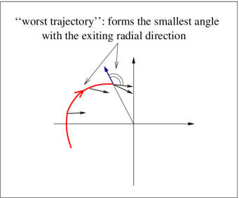
It is clear that the worst trajectory always rotates clockwise around the origin when $\delta_{A_{i}}\leq 0$ for some $i\in\{0,1\}$. If $\delta_{A_{i}}>0$ for $i=1,2$ then the eigenvectors of $A_{1}$ are $(1,1)^{T}$ and $(1,-1)^{T}$, while the eigenvectors of $A_{2}$ are $(1,F)^{T}$ and $(1,-F)^{T}$. In this case it is easy to check that $m_{1}m_{2}<0$ and therefore, from Lemma 5, without loss of generality we can assume

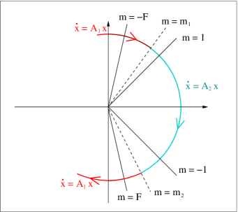
$$F<m_{2}<-1<1<m_{1}<-F.$$

Figure 2: Construction of the worst trajectory in the case $\delta_{A_{1}}>0,\ \delta_{A_{2}}>0$

As a consequence $D_{1}$ and $D_{2}$ divide the space into four connected components, each one intersecting the eigenspace of exactly one among $A_{1}$ and $A_{2}$. This implies that also in this case the worst trajectory rotates clockwise around the origin. This trajectory is the concatenation of integral curves of $A_{2}x$ from points of $D_{1}$ to points of $D_{2}$ and integral curves of $A_{1}x$ from points of $D_{2}$ to points of $D_{1}$ (see Figure 2).

As explained in the previous papers [1, 3] the behaviour of the worst trajectory is sufficient to derive the stability properties of (1). Let us analyse the worst trajectory $\gamma_{x_{0}}(\cdot)$ where $x_{0}\in D_{i}$. Assume that $T>0$ is such that $x_{1}=\gamma_{x_{0}}(T)$ is the first intersection point between the worst trajectory and $D_{i}$. The worst trajectory tends to the origin as time goes to infinity if and only if $\mathcal{R}:=|x_{1}|/|x_{0}|<1$, and in this case the system is GUAS (see Figure 3 (a)). It is periodic if and only if $\mathcal{R}=1$, and in this case the system is uniformly stable but not GUAS (see Figure 3 (b)). It blows up if and only if $\mathcal{R}>1$, and in this case the system is unbounded (see Figure 3 (c)).

Figure 3: The worst trajectory: meaning of the function $\mathcal{R}$

The computation of $\mathcal{R}$ was done in details in [1, 3]. The formula which is given in Section 2 is a simpler reformulation of the ones previously obtained, in terms of our invariants. This concludes the proof of S4.

References

• [1] M. Balde and U. Boscain. Stability of planar switched systems: the nondiagonalizable case. Commun. Pure Appl. Anal., 7(1):1–21, 2008.
• [2] F. Blanchini and S. Miani. A new class of universal Lyapunov functions for the control of uncertain linear systems. IEEE Trans. Automat. Control, 44(3):641–647, 1999.
• [3] U. Boscain. Stability of planar switched systems: the linear single input case. SIAM J. Control Optim., 41(1):89–112 (electronic), 2002.
• [4] W. P. Dayawansa and C. F. Martin. A converse Lyapunov theorem for a class of dynamical systems which undergo switching. IEEE Trans. Automat. Control, 44(4):751–760, 1999.
• [5] D. Liberzon. Switching in systems and control. Systems & Control: Foundations & Applications. Birkhäuser Boston Inc., Boston, MA, 2003.
• [6] M. Margaliot and G. Langholz. Necessary and sufficient conditions for absolute stability: the case of second-order systems. IEEE Trans. Circuits Syst.-I, 50:227–234, 2003.
• [7] P. Mason, U. Boscain, and Y. Chitour. Common polynomial Lyapunov functions for linear switched systems. SIAM J. Control Optim., 45(1):226–245 (electronic), 2006.
• [8] A. P. Molchanov and E. S. Pyatnitskiĭ. Lyapunov functions that define necessary and sufficient conditions for absolute stability of nonlinear nonstationary control systems. I. Automat. Remote Control, 47(3):343–354, 1986.
• [9] A. P. Molchanov and E. S. Pyatnitskiĭ. Lyapunov functions that define necessary and sufficient conditions for absolute stability of nonlinear nonstationary control systems. II. Automat. Remote Control, 47(4):443–451, 1986.
• [10] R. Shorten and K. Narendra. Necessary and sufficient conditions for the existence of a common quadratic Lyapunov function for two stable second order linear time–invariant systems. In Proceedings 1999, American Control Conf., pages 1410–1414, 1999.