Self-replicating Functions and the Renormalization Group

Abstract

The partial success of the block renormalization group techniques is analysed in terms of a functional operator which formalizes the idea of self-replicability of a system in terms of smaller blocks which are similar to the original. The mathematical properties of the fixed points of this transformation are analyzed.

I Introduction

The renormalization group (RG) is one of the most relevant theoretical tools in many branches of physics. Its main idea is that studying the changes of behaviour of a system under a scale transformation can provide very useful information. Kadanoff gave the most successful mental image when he developed the idea of block spins Kadanoff (1966). Consider a 2D lattice of interacting spins, and split it into $2\times 2$ blocks. Each block, under some conditions, behaves like a single spin, only varying the coupling constants which quantify the interaction.

In this spirit, the block renormalization group (BRG) starts its procedure by finding the ground state of a hamiltonian on a small system. Then, various systems of the same type are put into contact, making up a block, and the ground state of the same hamiltonian on the global system is searched variationally using as building bricks the ground states for each part. Then, the full procedure is iterated until we obtain the ground state for a system of the desired size. Changing the point of view, we may say that the ground state of a big system is approximated, variationally, using as building bricks the ground states for each of its parts.

The BRG has met variable success in practice. The practicioners abandoned it in favour of other methods, such as the density matrix renormalization group (DMRG), a RG technique of high accuracy, but which lacks some important features of the RG, such as the intimate relation between fixed points and critical systems White (1993); Vidal (2007). These conceptual problems encouraged a return to the analysis of the BRG, in order to understand the reason of its failures and successes. This study led to the development of the correlated blocks renormalization group (CBRG) by Martín-Delgado et al., which was rather successful for problems in quantum mechanics in 1D and 2D, but for unclear reasons Martin-Delgado et al. (1996).

In this work we introduce a functional transformation which explains the outcome of a BRG prescription in the case of single-body quantum mechanics (i.e.: obtaining the ground state of a hamiltonian acting on square integrable functions on a subset of $\text{\bf R}^{n}$), which we call the replica transformation. In intervals of R, it acts following these steps. First of all, we generate two scaled-down copies of the original function, and place them on the left and right halves of the interval. Now we find the best approximation to the original function within the subspace spanned by these two. Once normalized, this best approximation is the replicated function, and the scalar product with the original will be called the self-replicability of the function.

Once this operation is generalized to sets of functions, we show that a BRG prescription, such as the CBRG, is successful whenever the low energy spectrum of the hamiltonian on each block constitute an approximately self-replicable set. The CBRG attained success by playing with the boundary conditions between the blocks in such a way that this requirement was fulfilled.

This article is organized as follows. Section II introduces our model problem, i.e.: to obtain the low energy spectrum of the hamiltonian of a free particle in an interval, along with a naive BRG analysis and the explanation of its failure. In section III the CBRG prescription is reviewed. Section IV introduces formally the replica transformation and the self-replicability parameter, both for individual functions and for sets of them. In section V we prove some rigorous results about self-replicable sets of functions. We conclude in section VI, summarizing the results and providing some hints for future developments, such as the extension to many-body problems.

II Model problem and BRG approach

II.1 Model problem

Our model problem was originally formulated by K.G. Wilson as a toy model in order to dilucidate the reason of the failures of the BRGWhite (1999). We are asked to obtain the low-energy spectrum of the free hamiltonian for a spinless particle in a 1D box. In mathematical terms, the lowest eigenstates of the laplacian on an interval. The configuration space is discretized into a graph. Then, the hamiltonian becomes a $N\times N$ matrix related to the discrete laplacian on it: $H_{i,i-1}=H_{i-1,i}=-1$, $H_{i,i}=2$, for $i>1$ and $i<N$. The boundary conditions (bc) are specially important. The discrete analogue of the fixed boundary conditions is equivalent to setting $H_{1,1}=H_{N,N}=2$, while for free boundary conditions we have $H_{1,1}=H_{N,N}=1$.

The problem can be generalized to an arbitrary graph ${\cal G}$. Then, the hamiltonian of a particle with free boundary conditions is just $H_{free}=D-A$, where $D$ is the diagonal matrix in which the entry of each vertex is its degree, and $A$ is the adjacency matrix, i.e.: $A_{ij}=1$ if there is a link between sites $i$ and $j$, and zero otherwise. Fixed boundary conditions have a less natural generalization. If the graph vertices have uniform bulk degree $d$, then $H_{fixed}=dI-A$. A potential energy can be included by adding some $V_{i}$ to the diagonal elements. In absence of such a potential, both $H_{free}$ and $H_{fixed}$ are positive defined for any graph. It can be easily proved that $H_{free}$ has a homogeneous zero mode for every possible graph.

Of course, there are more physical problems which lead to the same mathematical formulation, e.g.: a vibrating string or a tightly bound electron in a lattice.

II.2 BRG approach to the problem

Let us consider two 1D lattice segments, of $N$ sites each. The ground state of the fixed bc hamiltonian is known for each of them. Now we attempt to obtain a variational estimate of the ground state of the compound segment using arbitrary linear combinations of the ground states of each block as Ansatz.

In more explicit terms, let $\psi^{N}_{0}$ be the exact ground state for $N$ sites. Now we define $\psi^{L}$ and $\psi^{R}$ to be the natural extensions to the lattice of $2N$ sites: $\psi^{L}_{i}=(\psi^{N}_{0})_{i}$ if $i\leq N$, and zero otherwise, while $\psi^{R}_{i+N}=(\psi^{N}_{0})_{i}$ if $i\leq N$, and zero otherwise also. Now we build a variational Ansatz, $\psi=\alpha_{L}\psi^{L}+\alpha_{R}\psi^{R}$ and get an effective hamiltonian for these two states. Let $H_{t}$ be the full hamiltonian for the composite lattice. Now, using Dirac’s bra-ket notation, we get

$$H_{eff}=\begin{pmatrix}\left<\psi^{L}\right|H_{t}\left|\psi^{L}\right>&\left<\psi^{L}\right|H_{t}\left|\psi^{R}\right>\cr\left<\psi^{R}\right|H_{t}\left|\psi^{L}\right>&\left<\psi^{R}\right|H_{t}\left|\psi^{R}\right>\cr\end{pmatrix}$$ (1)

The problem, therefore, reduces to the diagonalization of this $2\times 2$ effective hamiltonian matrix, $H_{eff}$. Variational approaches are always highly dependent on the quality of the Ansatz. In this case, the results prove it to be surprisingly inadequate. The BRG approximation to the ground state energy of the $40$ sites lattice is $E^{(0)}_{20+20}\approx 0.202$, while exact diagonalization gives $E^{(0)}_{40}\approx 0.00587$. This means an error $400\%$. The cause of the failure is apparent when we plot, in figure 1, the wavefunctions of the exact ground state for $N=40$ sites and the best approximation within the BRG Ansatz.

Figure 1: Above: the exact ground states of the $N=20$ systems. Below: the best approximation within the BRG Ansatz.

The boundary conditions force the wavefunctions to take the value zero at the borders of each block, thus making a spurious kink appear in the center of the complete system. On the other hand, if we make the same experiment with free bc, the result is completely satisfactory, but in a trivial way. Both $\psi^{L}$ and $\psi^{R}$ are homogeneous, and so is the global ground state. Therefore, the first lesson to be obtained is that boundary conditions may be determinative for the failure of a RG-prescription.

III Review of the correlated blocks RG

A successful real space prescription for this problem which respected the BRG spirit was given by Martín-Delgado et al.Martin-Delgado and Sierra (1995); Martin-Delgado et al. (1996). We will describe briefly the method in this section. A thorough explanation of the method can be found in the PhD dissertation of one of the present authors Rodriguez-Laguna (2002).

Let us consider a linear chain of $N$ sites. We will split this chain into $N_{b}=2^{k}$ blocks of $m$ sites each, for some integer $k$. Each block is labeled by the index $p\in[1..N_{b}]$, isolated from the others and given free boundary conditions. It will have, therefore, a certain self-interaction hamiltonian $A_{p}$. We obtain the low energy eigenstates of these self-interaction hamiltonians and, with them, we build a chain of Ansätze, which we will describe henceforth.

First of all, we write down the effective hamiltonian for two neighbouring blocks, using the $2m$ states as variational bricks. The global bc will again be set to be free, but in order to reproduce correctly the link between them we need two types of operators. Following Martín-Delgado et al.Martin-Delgado et al. (1996), we define influence operators as those which restore the correct boundary conditions between the two blocks and interaction operators as those which take into account the dynamical aspect of the joining.

This superblock hamiltonian, or level-2 block, is now diagonalized exactly, and we retain, out of the $2m$ eigenstates, the $m$ with lowest energy. Those states will represent the block as we proceed to the next RG step. Now two such level-2 blocks are put together, and the same process is repeated. The RG iteration continues until the full system is contained in a single superblock.

The same technique works, with very reasonable success, with fixed boundary conditions, in presence of a potential or, with the necessary generalizations, in the 2D case. A reference which describes the technical details is the PhD dissertation of one of the authors Rodriguez-Laguna (2002).

IV Self-replicability

The main thesis of this work is the following: the reason for the success of the CBRG prescription, as described in the previous section, is the special self-similar properties of the eigenfunctions of the hamiltonian when free boundary conditions are applied.

Given a (normalized) function $\phi\in L^{2}[0,1]$, let us define the operators $L$ and $R$ as:

$$L\phi(x)=\begin{cases}\sqrt{2}\;\phi(2x)&\text{if $x<1/2$}\\ 0&\text{if $x\geq 1/2$}\end{cases}$$

$$R\phi(x)=\begin{cases}0&\text{if $x<1/2$}\\ \sqrt{2}\;\phi(2x-1)&\text{if $x\geq 1/2$}\end{cases}$$

i.e.: they return reduced copies which are similar to the original function for each part (left and right), and the $\sqrt{2}$ factor is included so that $L\phi$ and $R\phi$ have the same $L^{2}$ norm as $\phi$. We may try to reproduce the original $\phi$ within the subspace spanned by $L\phi$ and $R\phi$. Is this possible?

Let us consider all functions to be $L^{2}$-normalized and let us define the replica transformation:

$${\cal R}\phi={\cal N}\left[\;\left<\phi|L\phi\right>\,L\phi+\left<\phi|R\phi\right>\,R\phi\;\right]$$ (2)

where ${\cal N}$ is a normalization constant. Since $\left<L\phi|R\phi\right>=0$, this is the best approximation to the original function within the given subspace. Its accuracy shall be given by the parameter

$$S\equiv\left<{\cal R}\phi|\phi\right>$$ (3)

where the symbol $S$ stands for self–replicability. The value $1$ means perfect, and $0$ means that the two states are orthogonal.

The procedure is easily extended to sets of functions or, better, to functional subspaces. Let us denote any such set, with $m$ functions, as $\phi\equiv\{\phi_{i}\}_{i=1}^{m}$, which we will assume to constitute an orthonormal set in $L^{2}[0,1]$. These functions are approximated within the subspace spanned by the $2m$ functions $\{L\phi_{i},R\phi_{i}\}_{i=1}^{m}$, which also make up an orthonormal set. All the $2m$ functions, $L\phi$ and $R\phi$ contribute to the reconstruction of the parent wavefunctions $\phi$. We can give a preliminary definition of the replica transformation as

$${\cal R}_{0}\phi_{i}=\sum_{j}\left(\alpha_{ij}L\phi_{j}+\beta_{ij}R\phi_{j}\right)$$ (4)

where the matrices $\alpha$ and $\beta$ are given by the scalar products

$$\alpha_{ij}=\left<\phi_{i}|L\phi_{j}\right>\qquad\beta_{ij}=\left<\phi_{i}|R\phi_{j}\right>$$ (5)

We should emphasize that the replica transformation acts on functional subspaces. The considered initial set of $m$ functions is just a basis for the relevant subspace, and equation [4] for the best approximation is correct only if the basis is orthonormal. The scalar products among the elements of the replicated set ${\cal R}_{0}\phi$ are given by

$$\left<{\cal R}_{0}\phi_{i}|{\cal R}_{0}\phi_{j}\right>=$$

$$=\sum_{k}\left<\phi_{i}|L\phi_{k}\right>\left<L\phi_{k}|\phi_{j}\right>+\left<\phi_{i}|R\phi_{k}\right>\left<R\phi_{k}|\phi_{j}\right>$$

Let us remind that $\sum_{k}\left|L\phi_{k}\right>\left<L\phi_{k}\right|$ is a projector on the subspace of the left copies, so we define projector $P_{LR}$ on the full subspace spanned by the set $\{L\phi_{i},R\phi_{i}\}$, and observe that

$$\left<{\cal R}_{0}\phi_{i}|{\cal R}_{0}\phi_{j}\right>=\left<\phi_{i}|P_{LR}|\phi_{j}\right>$$ (6)

Therefore, the replicated functions are orthogonal if and only if the operator $P_{L,R}$ acts trivially on the original set, i.e.: if the functions are self-replicating. Otherwise, we must apply a Gram-Schmidt procedure, let us call it $G$. This way, the we define the full replica transformation as:

$${\cal R}\phi=G{\cal R}_{0}\phi$$ (7)

In order to perform numerical experiments, we should also define the transformation for discretized functions. We will assume that ${\cal R}$ acts internally on a certain discrete functional space, isomorphous to $\text{\bf R}^{N}$. Therefore, when applying the $L$ and $R$ operators, two values of the old function must fit into a single new value. The most symmetric way of doing this is the local averaging:

$$(L\phi)_{i}=\begin{cases}{1\over 2}(\phi_{2i-1}+\phi_{2i})&\text{if $i\leq N/2$}\cr 0&\text{otherwise}\cr\end{cases}$$ (8)

along with an equivalent formula for the right side.

The generalization to higher dimensions does not pose any theoretical difficulty. In 2D, e.g., functions are defined in the unit square, which is divided into four regions. Each function gives rise to four children, out of which we shall attempt its reconstruction.

Another possible generalization is the choice of a Hilbert space different from $L^{2}$. By choosing a Sobolev space, we ensure that the replicated function and the original one are not only similar in value, but also in derivatives. This can be an important issue, as will be seen in the next section.

IV.1 Numerical Experiments in 1D

Let us apply the replica operator to the ground state of the laplacian with fixed bc on a 1D lattice. The best approximation is given in figure 2. Here $S$ takes the value $0.8488$, which is not too bad (with a Sobolev-type norm, it would be much lower), but it gets worse as the replica operator is iterated. Figure 3 shows us the second, third and fifteenth iterations. After some iterations the finite resolution of the computer yields a quasi-constant function as approximation. This function is exactly self-replicable.

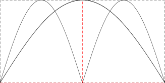
Figure 2: The ground state of a 1D laplacian with fixed b.c. is not self–replicable.

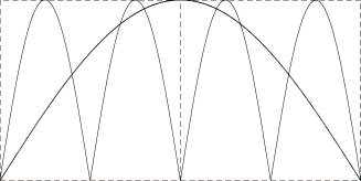
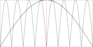
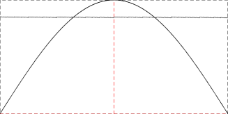
Figure 3: The procedure is iterated. The last box represents the fifteenth iteration.

As another example, let us consider the low energy spectrum of the 1D laplacian with free bc. It is self-replicable to a reasonable approximation, although not exactly, as shown in figure 4.

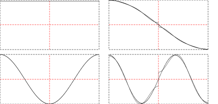
Figure 4: A single step of the replica transformation on the lowest energy states of the free bc laplacian.

The $S$ parameters are $1$, $0.9996$, $1$ and $0.9957$. This means that the ground state (flat) and the third states are exactly reproduced. Analysis of the weights shows that:

$\bullet$

The first state is absolutely self-replicable by itself.

$\bullet$

The second consist of two copies of itself, the first one raised and the second one lowered, using the first state to this purpose. The finite slope at the origin is not correctly represented.

$\bullet$

The third state only requires two copies of the second one.

$\bullet$

The fourth state is even more interesting. Both the left and the right parts are a combination of the second and third states. The finite slope at the origin is again incorrectly represented.

The procedure may be easily iterated without excessive distortion. The results are shown in figure 5. These functions have a rough look, but factors $S$ are not too different: $1$, $0.9996$, $0.9996$ and $0.9949$.

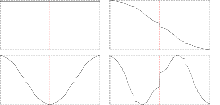
Figure 5: The same functions as in figure 4 after 15 iterations (once the fixed point has been reached).

It is also illuminating to perform the same experiment on the four lowest energy states of the fixed bc laplacian (see figures 6 and 7). The values of the $S$ parameters at the first iteration are not excessively bad: $0.9537$, $1$, $0.9452$ and $1$ (to four digits). But the fixed point yields very different numbers: $0.8431$, $0.8724$, $0.8516$ and $0.8020$.

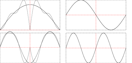
Figure 6: The lowest energy states of the fixed b.c. laplacian after one iteration.

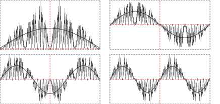
Figure 7: The same functions as figure 6, once the fixed point has been reached (15 iterations).

There is a great wealth of fixed points of this transformation, but most of them are non-smooth and have non-trivial fractal properties. Numerical experiments led immediately to a smooth family of exactly self-replicating functions: the polynomials. If we apply the Gram-Schmidt procedure on $\{1,x,x^{2},\cdots,x^{m}\}$, it is easily checked numerically that the self-replicability parameter is exactly one for all the functions. The meaning of this result will be explained in detail in section V.

IV.2 Numerical Experiments in 2D

As it was previously stated, the process may be easily generalized to 2D, if instead of splitting the interval into two regions we part it into four. The case of the eigenfunctions of the free b.c. laplacian yields a fixed point which is much smoother than in the 1D case, as it is shown in figure 8. In the fixed bc case, we obtain a rather different fixed point, as it is shown in figure 9. Among the fixed points we have found a great richness of structures. Figure 10 shows a familiar pattern.

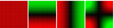
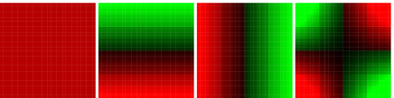
Figure 8: Above, wave-functions for the 2D laplacian with free b.c. for a $32\times 32$ system. Below, the fixed point we reach. These last functions are also smooth.

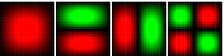
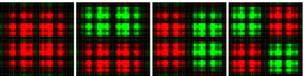
Figure 9: Same concept as in figure 8, but for initial wave-functions with fixed bc. The fixed point is thoroughly different.

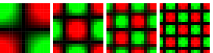
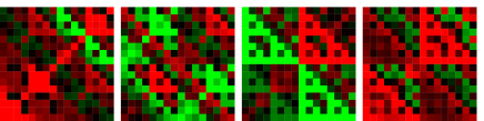
Figure 10: $16\times 16$ Wave-functions of higher energy than the previous ones, which yield a repeated pattern based on the Pascal or Sierpiński triangle. It must be remarked that this curious structure is not stable, and that it is due to a slight asymmetry of numerical origin in the initial states.

V Analytical Functions and Self-Replicability

A very simple argument shows that the only self-replicable function on an interval which is analytical is the uniform function. The replicated function can be always written as

$${\cal R}\phi(x)=\alpha\chi_{[0,1/2]}(x)\phi(2x)+\beta\chi_{[1/2,1]}(x)\phi(2x-1)$$ (9)

where $\chi_{[a,b]}(x)$ is the characteristic function for the interval $[a,b]$.

The self-replicability condition is $\phi(x)={\cal R}\phi(x)$. Then, obviously, $\phi(0)={\cal R}\phi(0)$, from where we deduce that $\alpha=1$. Now we force the equality of all the derivatives at that point: $\phi^{(k)}(x)={\cal R}\phi^{(k)}(2x)=2^{k}\phi^{(k)}(2x)$ in $[0,1/2]$. Now, picking up the point $x=0$ again, we get $\phi^{(k)}(0)=2^{k}\phi^{(k)}(0)$, which proves that all the derivatives of the function are zero at the origin so, if the function is analytical, it must be a constant.

A more interesting result is obtained when we analyze the self-replicability of a set of functions (equivalently, of a subspace). According to equation [7], we can extend the previous argument in the following way. Restricting ourselves to the left interval $[0,1/2]$, the self-replicability condition reads

$$\sum_{j}\alpha_{ij}\Phi_{j}(2x)=\Phi_{i}(x)$$ (10)

Let us assume that the functions $\phi_{j}$ are analytical. Then, derivating $k$ times that expression with respect to $x$ we obtain

$$\sum_{j}\alpha_{ij}\Phi_{j}^{(k)}(2x)={1\over 2^{k}}\Phi_{i}^{(k)}(x)$$ (11)

Restricting ourselves to the point $x=0$, that equation reads

$$\sum_{j}\alpha_{ij}\Phi^{(k)}_{j}(0)={1\over 2^{k}}\Phi^{(k)}_{i}(0)$$ (12)

Let us assume that $\Phi^{(k)}(0)\neq 0$ for all $k$. Then, equation [12] implies that matrix $\alpha_{ij}$, which is finite, has an infinite set of eigenvalues, $1/2^{k}$ for all positive $k$. Since that can not happen, we have proved that, if $k>m$, the derivatives must vanish. In other terms, all the $\phi_{i}$ must be polynomials.

It easy to prove that the subspace spanned by $\{1,x,x^{2},\cdots,x^{m}\}$ is self-replicating. Both results together allow us to state the following theorem: the only analytical family of self-replicating functions are the polynomials.

VI Conclusions

Let us return to the original question: why do the free bc CBRG work, while if we try fixed bc the failure is complete? The reason is that the eigenfunctions of the free bc hamiltonian make up an approximately self-replicable set, because they resemble the polynomials.

So, the success of a BRG approach requires the building bricks to be suitable for the problem at hand. The boundary conditions, being the main freedom of the RG practicioner, should be chosen with care. But the main guide should be this: make the block eigenfunctions as close to self-replicability as possible.

To summarize, we have introduced the replica transformation on a functional space, which attempts to reproduce a function or set of functions by the best approximation attainable with reduced and scaled copies of itself. We have defined the self-replicability parameter as a measure of the failure of a function to replicate itself. Some numerical experiments have shown the complex structure of the set of fixed points of this transformation, although a proof has been provided that most of them are non-smooth functions: only the polynomials, up to any order $n$, constitute an analytical self-replicable set.

The idea of self-replicability was used to explain the success of the CBRG, because it uses free boundary conditions in order to split the blocks. This choice is appropriate because the eigenfunctions of the laplacian with those bc are approximately self-replicating.

A very interesting line of further work would be to study the possible extension of these ideas to other problems where real space RG has been applied, such as many-body hamiltonians. The splitting of the system into blocks should be done in such a way that the resulting eigenfunctions of the block hamiltonian are approximately self-replicable. This poses an interesting challenge with immediate applicability to the development of numerical methods in condensed matter and particle physics.