Water in the Near IR spectrum of Comet 8P/Tuttle

Abstract

High resolution spectra of Comet 8P/Tuttle were obtained in the frequency range 3449.0–3462.2 cm^-1 on 3 January 2008 UT using CGS4 with echelle grating on UKIRT. In addition to observing solar pumped fluorescent (SPF) lines of H₂O, the long integration time (152 minutes on target) enabled eight weaker H₂O features to be assigned, most of which had not previously been identified in cometary spectra. These transitions, which are from higher energy upper states, are similar in character to the so-called ‘SH’ lines recorded in the post Deep Impact spectrum of Comet Tempel 1 (Barber et al., 2007).We have identified certain characteristics that these lines have in common, and which in addition to helping to define this new class of cometary line, give some clues to the physical processes involved in their production. Finally, we derive an H₂O rotational temperature of $62\pm 5\,\mathrm{K}$ and a water production rate of $(1.4\pm 0.3)\times 10^{28}$ molecules s^-1.

1 Introduction

Cometary nuclei are the most primitive objects in the solar system. Within about 3 AU of the sun, solar heating causes the surface temperature of the nucleus to rise above 200 K; water ice sublimes and other volatiles and icy dust grains are expelled from the surface. The motion, chemistry and rate of sublimation of molecules from the icy grains are influenced by the solar wind and solar radiation. Initially the escaping gases form a dynamic, gravitationally-unbound atmosphere, the coma. They are subsequently swept into the comet’s plasma and dust tails and eventually dissipate into interplanetary space. The surface of the nucleus is processed during the course of repeated visits to the inner solar system, becoming covered with a rubble blanket of particles too large to be dragged away by escaping gas. During the course of numerous perihelia, the outer surface becomes completely depleted of volatile materials which either escape from the surface or else migrate inwards. This creates an outer mantle of siliceous dust (Huebner, 2008), above a layered structure in which the more volatile species are found at greater depths (Prialnik et al., 2008). This structure results in the great variety that is observed in active comets.

Cometary nuclei typically have radii of $\sim$3 km and are not able to be resolved from Earth. During close approaches, the inner coma of some comets are resolvable with large terrestrial instruments. However, in general, data obtained with Earth-based instruments are indicative of conditions in a wider region of the coma, and our understanding of conditions within the inner coma (a region extending up to a few hundred km, where energy transfer is collisionally-dominated, relies largely on modelling. Our understanding of the more extended regions of the coma, where the densities of the species are too low for thermodynamic equilibrium to exist, also relies on modelling. In particular, models of cometary coma predict the existence of so-called ‘solar pumped fluorescent’ (SPF) H₂O emission lines. These originate from ro-vibrational excited upper states of the molecule, which, if observed in a collisionally-dominated region would be characteristic of kinetic temperatures of several thousand K, but are able to be produced in the cold, rarefied conditions existing in cometary coma, since these excited states, which have relatively large Einstein A coefficients, have time to decay radiatively before they are de-excited by collision with another molecule.

Despite the success of models in predicting SPF lines (Crovisier, 1984; Weaver and Mumma, 1984, Mumma et al., 1995), the physical conditions existing in cometary coma are highly complex and recent observations of Comet Tempel 1 (Barber et al., 2007) revealed a type of emission line, not previously recorded in cometary spectra, and not predicted by the existing cometary models. These so-called ‘SH’ lines originate from upper states that are excited to higher vibrational energies than are the upper states of the SPF lines. Consequently, their production mechanisms are not able to be explained simply, by the existing cometary models. The near-Earth approach of Comet 8P/Tuttle in January 2008, provided an opportunity for us to search for, assign and characterise SH emission lines in its coma. We believe that our findings, which are presented in this paper, provide the basis for a more thorough investigation of the physical processes involved in the production of SH lines in cometary coma.

2 Comet 8P/Tuttle

8P/Tuttle is a short period comet, P_orb = 13.51 yr, and is the parent of the Ursid meteor stream (Jenniskens et al., 2002). It had been estimated that the comet has a radius of $\sim$ 7.5 km, making it the largest of the group of 18 short period comets reported on by Licandro et al. (2000). However radar images obtained on 2-4 January 2008 (Harmon et al., 2008) show a bifurcated nucleus consisting of two lobes each 3–4 km in diameter, suggesting a possible contact binary. Photometric measurements, have yielded rotational times of the nucleus as being either 5.71$\pm$0.04 hr (Schleicher and Woodney, 2007b), 7.7$\pm$0.2 hr (Harmon et al., 2008), or multiplicities of 5.7 and 7.4–7.6 hr (Drahus et al., 2008). However, these results may need to be re-interpreted in the light of the probable bifurcation of the nucleus.

In the scheme proposed by Levison (1996), comets are classified by reference to the Tisserand invariant. To a first order, this parameter is a constant of the motion of a comet. It is based on the Jacobi integral in the restricted three-body problem (Tisserand, 1894; Moulton, 1947). Because 8P/Tuttle has a Tisserand invariant of less than 2 (T_J = 1.601), it is classified as a ‘near isotropic comet’ (NIC) of the Halley type. However, its present orbit is not characteristic of this class, since most NIC comets have long orbital periods (defined as being greater than 200 yr).

8P/Tuttle also differs from most short period comets as these normally have a Tisserand invariant 2 $\leq$ T_J $\leq$ 3 and in the Levison scheme are referred to as ‘ecliptic comets’ (EC).

Being a short period NIC, the chemistry of 8P/Tuttle is of particular interest. Unlike most short period comets, which are of the EC type, 8P/Tuttle is believed to have been formed in the region of the giant planets. It therefore has the potential to reveal possible differences between EC and NIC objects. Because it has made many approaches to the Sun, 8P/Tuttle’s surface may be highly processed like that of an EC. If then, despite having a highly-processed surface, its spectra reveal a chemistry that is more like that of NICs than of ECs, it may be possible to identify differences in the chemistries of various regions of the very early solar system.

Even though, with the exception of the 1953 approach, 8P/Tuttle had been seen on each orbit since its discovery in 1858, until recently there had been no detailed investigation of its near-IR spectrum. During the 2008 apparition, 8P/Tuttle approached to within 0.25 AU of the Earth and was favourably placed for observing (see for example, Bonev et al., 2008 and Böhnhardt et al., 2008).

3 Water in Cometary Spectra

In the near IR, the spectra of comets are rich in ro-vibrational H₂O emission lines which can, in principle, be observed from Earth. However, because of the low temperatures that characterise cometary comae, the strongest water lines are fundamental transitions (that is to say, transitions to ground vibrational states) from low-energy ro-vibrational states. Photons from these transitions are absorbed by water vapour in the Earth’s atmosphere, the molecules of which are in ground vibrational states.

Close to the nucleus the density is sufficiently great (generally upward of 10⁶ molecules cm^-3) to ensure that the molecules are collisionally thermalised in low J ground vibrational states, with a rotational temperature equal to the local kinetic temperature (Weaver and Mumma, 1984). There is no precise boundary between the collisionally-dominated and the less dense, radiatively dominated region, as the breakdown of thermal equilibrium occurs at different distances from the nucleus for each of the allowed rotational transitions between ground vibrational states. These distances vary between several tens of kilometres to several thousands of kilometres (Bockelée-Morvan, 1987). Moreover, beyond the region where H₂O–H₂O collisions are able, alone, to maintain local thermodynamic equilibrium (LTE) there is a region where the additional contribution of H₂O–electron collisions and line-trapping effects maintains LTE to greater radial distances (Bockelée-Morvan, 1987; Zakharov et al., 2007). In particular, Xie and Mumma (1992) showed that at distances of several thousand kilometres, e^-–H₂O collisions play an important role in exciting water molecules. In Section 7 we discuss a number of mechanisms, including e^-–H₂O collisions, that may possibly be involved in the formation of the so-called ‘SH’ water lines that were observed to be present in our 3 January 2008 UT spectrum of 8P/Tuttle. SH, or ‘stochastic heating’ lines were first identified in the ‘Deep Impact’ spectrum of Comet Tempel 1 (Barber et al., 2007), and were subsequently noted to be present in another spectrum of the same comet (Mumma et al., 2005, Figure 2). Their characteristics are discussed in Section 5.

At distances greater than a few thousand kilometres from the nucleus the density of the species is sufficiently low, and the mean free path between collisions large enough, for ‘fluorescence equilibrium’ to exist. That is to say, radiation is due to the balance between solar pumping to vibrationally-excited states and subsequent spontaneous radiative decay (Crovisier, 1984). Under collisionally-thermalised conditions, these upper states would typically require temperatures of several thousand Kelvin for them to be sufficiently populated for their collisionally-induced radiation to lower states to be observable. The observation in cometary spectra of transitions from vibrationally-excited upper states, indicates that they must be produced in regions where Boltzmann statistics do not apply.

When vibrationally excited states decay radiatively to lower energy ro-vibrational states above the ground vibrational state (hot bands), the photons emitted are not absorbed in the Earth’s atmosphere. Recognition of this fact was a key factor in developing the ‘solar-pumped fluorescent’ (SPF) approach to analysing cometary spectra (Mumma et al., 1995). Spectra containing these SPF transitions enable information to be derived about the rotational temperature, T_rot of the inner coma and the water production rate, Q${}_{\mathrm{H_{2}O}}$. A comparison of this latter value with the production rates of trace species provides the abundance ratios that are fundamental to understanding cometary chemistry.

Because the upper states populated by solar pumping are not collisionally thermalised, the derivation of physical quantities from line intensities requires knowledge of all the possible excitation as well as the alternative de-excitation routes. Each upper excited ro-vibrational state can be populated directly by radiative pumping of rotational levels of the ground vibrational state, as well as by cascade from higher energy states (Crovisier, 1984). The relative probabilities of these various upward and downward routes are temperature-dependent. Models have been developed to compute the g-factors for each SPF line, from which line intensities are able to be calculated as a function of temperature (Crovisier, 1984; Mumma et al., 1995, Dello Russo et al., 2000). These models require a knowledge of the Einstein A coefficients for the downward transitions. Ideally, the upward pumping rates should be computed using the Einstein B coefficients. However, for simplicity, the temperature-dependent vibrational band intensities are frequently used to compute the upward pumping rates. For example, Dello Russo et al.  (2004) used Einstein A coefficients from the BT2 synthetic water line list (Barber et al., 2006) to model g-factors for all the H₂O SPF transitions in the: $\nu$₁+$\nu$₃–$\nu$₁, $\nu$₁+$\nu$₃–$\nu$₃, 2$\nu$₁–$\nu$₁, 2$\nu$₁–$\nu$₃ and $\nu$₁+$\nu$₂+$\nu$₃–$\nu$₁–$\nu$₂ vibrational bands, from upper states having J $\leq$ 7.

The 2.9–3.0 $\mu$m (3300–3450 cm^-1) spectral region is particularly rich in SPF lines and is also largely devoid of other molecular species. The availability of accurate g-factors has enabled this region to be used in determining cometary rotational temperatures and water production rates (e.g. Dello Russo et al., 2004 and 2006).

4 Observations

We observed 8P/Tuttle on its approach to the Sun (perihelion being on 27 January UT), on the nights of 3, 4 and 5 January 2008 UT from UKIRT, Hawaii, using the echelle grating on CGS4. We report here on the spectra that we obtained on 3 January UT, in the frequency range 3 440.6–3 462.6 cm^-1. The heliocentric distance on this date was $\sim$1.09 AU, and the geocentric distance and velocity were $\sim$0.25 AU and $\sim$3.3 km s^-1 respectively; the latter figure corresponds to a red shift of 0.038 cm^-1, which was equivalent to 1 pixel on the array, and less than the minimum resolution of our instrument, which at R = 37 000 was 0.093 cm^-1 at 3 450 cm^-1. The total visual magnitude of 8P/Tuttle at the time of our observations was $\sim$5.8. However our observations were of the bright inner coma region which presented a point source in our instrument, and required long integration times.

We used a slit of 2-pixel width of length 90 arcsec, oriented east-west. The scale was 0.86 arcsec per pixel in the spatial direction (156 km at the comet) and 0.41 arcsec in the spectral direction, (149 km at the comet for a 2-pixel slit). The telescope was dithered to give 2x2 sampling every 40 seconds. Observations were acquired using a standard ABBA sequence, which was achieved by nodding the telescope 22 pixels along the slit. In this mode, the comet signal was present in both the A and B beams (rows 114 and 92 respectively), which, compared to nodding to blank sky, increased the signal to noise ratio by a factor of $\sqrt{2}$, when both signals were added using the (A-B)-(B-A) routine to remove the sky. Each ABBA series represented a total of 160 seconds integration time. Total time on-target was 152 minutes. Spectra of an A0V star, HD 6457, were obtained at the beginning and end of the observing session. Standard star spectra are required in order to adjust for frequency-dependent atmospheric transmission, and also to enable absolute flux calibration. Before dividing by the standard star, we removed high frequency noise from both the 8P/Tuttle and standard star data using Fourier transform smoothing. We rejected all data at frequencies where the atmospheric transmission was less than 20%, and this resulted in 19% of the data in the 3 440.6 to 3 462.6 cm^-1 range being excluded. We noted that transmission was poor at frequencies less than 3449.0 cm^-1 and above 3 460.2 cm^-1. We therefore decided to limit the spectral region under investigation to that lying between these frequencies. In this reduced, 11.2 cm^-1, frequency range less than 3% of the data failed to meet our 20% minimum atmospheric transmission requirement, and the average transmission in this reduced frequency range was 66%. After dividing by the standard star, flux calibration was achieved by multiplying the result by the frequency-dependent flux of HD 6457, calculated relative to Vega as a photometric 0.0 magnitude standard (Hayes, 1985), and assuming a black body function with T_eff = 9 480 K (Tokunaga, 2000, p151).

Because of the lack of arc lines in this spectral region, we frequency-calibrated our data using the position of several known SPF lines that were present in the 8P/Tuttle spectrum. This had the effect of transforming the observed spectrum into the rest frame. The fully-reduced, flux-calibrated spectrum is given in Figure 1.

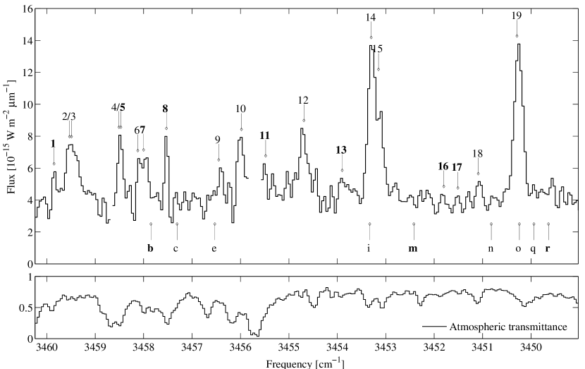
Figure 1: The upper chart shows the spectrum of Comet 8P/Tuttle, UT 3 January 2008 adjusted to rest frame and plotted after dividing by standard star HD 6457 (normalised) to adjust for frequency-dependent atmospheric transmission. The spectra of both the comet and standard star have been Fourier Transform smoothed to remove high frequency noise. Atmospheric transmission is shown in the lower chart, and no spectral data is displayed where transmission is less than 0.20. The figures above the spectrum indicate lines that have been assigned in Table 2, the numbering above the plot corresponds to that given in each entry in this table. Bold font is used to indicate SH transitions; SPF lines are numbered using normal weight font. The letters below the plot correspond to the nine SH lines which we would expect to be present in the spectrum (see text), but which were not positively identified. Their numbers correspond with those given in the first column of each entry in Table 3. Six of these either correspond to weak feature (S/N $\leq$ 2), or are at frequencies where they would be undetectable due to blending with stronger lines. Of the twenty-six SH lines listed in Table 3, we are unable to explain the absence of three, and these are identified with bold letters.

5 Data Analysis

We compared the features in Figure 1 with our BT2 database of H₂O SPF line positions and g-factors. Nine of these features are at frequencies corresponding to known SPF lines (there are actually eleven SPF lines, with two features being blends of two SPF lines). Details are given in Table 2. However, Figure 1 also includes a number of other features, whose shape and intensity above the continuum (S/N $\geq$2) suggest that they are spectral lines, rather than noise, but whose frequencies do not correspond to SPF lines.

In order to assign these other features, we employed the methodology detailed in Barber et al. (2007) for the identification of non-SPF features in the post Deep Impact spectrum of Comet Tempel 1. Initially we used the BT2 line list to generate synthetic emission spectra for water at a temperature of 3 000 K in the 3 449.0–3 462.2 cm^-1 frequency range, restricting the value of J for the upper state to 8, and the intensity of the weakest line to be generated was limited to 10^-3 of the strongest. The output, which consisted of about 600 individual lines was convolved to match the resolving power of the CGS4 echelle, R=37 000.

Some of the features in this synthetic spectrum are at frequencies corresponding to features in the spectrum of 8P/Tuttle. However, the relative intensities of the features in the observed and synthetic 3 000 K spectra do not agree. The reason is that the observed emission lines originate in low-density regions where vibrationally-excited upper states have sufficient time to decay radiatively before they can be collisionally de-excited. These upper states are populated by pumping low-lying rotational states and by cascade from higher levels (of which there will be many, most of which contribute little and can therefore be disregarded). Since the water molecules are not collisionally thermalised, the populations of the upper states can be substantially greater than would be the case if Boltzmann statistics applied, and the frequencies and intensities of the emissions from these states are frequently similar to those of emission lines from H₂O vapour in LTE regions at temperatures of, say, 3 000 K.

Our synthetic spectrum contains many more features than are present in the spectrum of 8P/Tuttle. It is therefore important to try to identify specific characteristics of the observed lines that differentiate them from lines in the synthetic spectrum that are absent in the observed spectrum.

When synthetic spectra are generated using BT2, one of the output files gives the frequency, assignment, intensity, Einstein A coefficient and lower state energy of every water transition in the frequency range, down to a specified intensity cut-off. Using these data, we were able to identify certain characteristics of those lines in our synthetic spectra whose positions matched those of features in the observed spectrum, that differentiated them from those that did not. This information enabled us to constrain the parameters applied when generating the BT2 synthetic spectrum, which reduced the number of lines in the synthetic spectrum and hence the risk of confusing noise and real spectral lines.

Before detailing these tighter parameters and our findings, we comment briefly on the ro-vibrational states of water. The three vibrational modes of the H₂O molecule, $\nu_{1},\nu_{2}$ and $\nu_{3}$ (symmetric stretch, bend and asymmetric stretch respectively), require different amounts of energy for one quanta of excitation. Also, the magnitude of each increment decreases as the total internal energy of the excited molecule increases. In the energy range in which we are interested, each quanta of symmetric and asymmetric stretch represents $\sim$3 400-3 700 cm^-1. These values are approximately twice the energy of one quanta of bend. Hence it is convenient to talk in terms of ‘polyads’, where each polyad, designated $\nu$ is the equivalent of one quanta of stretch or two of bend. Single bend quanta are denoted by ‘$\delta$’.

We noted that all the SPF lines in the observed spectrum came from the 2$\nu$ polyad, whilst the large majority of non-SPF lines that matched features in our synthetic spectra, were from the 3$\nu$ and 3$\nu$+$\delta$ polyads. We also noted that none of the upper states had more than two $\nu_{\mathrm{2}}$ quanta. In addition, the lines in our synthetic spectrum that corresponded to non-SPF features in Figure 1 all had Einstein A coefficients $\geq$ 1.0 s^-1, and were on average higher than those of the SPF lines, the average A_if being 23.0 and 7.4 s^-1 respectively. The SPF lines had upper states with energies in a very narrow range: 7 242–7 613 cm^-1, whilst the non-SPF lines had upper states with energies in the range 10 365 –12 940 cm^-1.

Rotational excitation, also affects which lines are observed in cometary spectra. This is defined in terms of the asymmetric top labels, $J,\ K_{\mathrm{a}},\ K_{\mathrm{c}}$ which represent total angular momentum and the prolate and oblate levels respectively. We designate ro-vibrational states ($\nu_{1}\ \nu_{2}\nu_{3}$)[$J\ K_{\mathrm{a}}\ K_{\mathrm{c}}$] and when assigning transitions, give the upper state first.

An examination of the $\sim$ 600 transitions in our synthetic spectrum revealed that none of the features in the spectrum of 8P/Tuttle corresponded to lines whose upper state had J $\geq$ 5. We also noted that none of the lines in our observed spectrum,assigned in Table 2, correspond to very weak features in our synthetic spectrum. They all correspond to lines in our synthetic spectrum having intensities greater than $\sim$0.5% of the intensity of the strongest line in the synthetic spectrum. In all of these respects the non-SPF lines that we identified in the spectrum of 8P/Tuttle had the same characteristics as the SH lines observed in the ‘Deep Impact’ spectrum of Comet Tempel 1 (Barber et al., 2007).

This information provided us with with a second, even tighter, set of parameters with which to search for SH lines. We produced a second synthetic BT2 spectrum with the constraints: J $\leq$ 5, 3$\nu$ or 3$\nu$+$\delta$ polyad, A_if $\geq$ 1.0 s^-1 and a minimum intensity cut-off equivalent to 0.5% of the intensity of the strongest line in the frequency range. Also we lowered the temperature of the synthetic spectrum to 2 500 K, which further reduced the total amount of data generated.

Although it still includes all the SPF lines that were present in our observed spectrum, this second synthetic LTE spectrum contains only 26 possible SH lines. Using these data, we were able to assign seven unblended SH lines in the observed spectrum. These are detailed in Table 2, which also gives E_upper, A_if; the type of transition, SPF or SH; the nuclear spin species identity (ortho/para) and the estimated signal-to-noise ratio of the lines. In addition to the unblended SH lines, we identified a feature centred at 3458.49 cm^-1. There is a known SPF line, (200)[423]-(100)[432], at 3458.51 cm^-1. However, at 62 K, the g-factor for this line is only 8.2$\times 10^{-10}$, which equates to a line of only $\sim$3% of the intensity of the feature observed at 3 458.49 cm^-1. The BT2 synthetic spectrum contains only one other water line in the 3 458.49 cm^-1 region, an SH line, (022)[432]-(120)[541] at 3458.47 cm^-1. We therefore conclude that this line is also present in the observed spectrum of Comet 8P/Tuttle, which represents an eighth SH detection.

Barber et al. (2007) assigned two unblended SH transitions in the spectrum of Comet Tempel 1 at 3 453.39 and 3 451.51 cm^-1 and a feature at 3 453.90 cm^-1 which they suggest might be a blend of two lines: (211)[322]–(210)[221], which has a 3$\nu$+$\delta$ polyad upper state, of energy 12 354 cm^-1 and (103)[110]–(102)[110], which has a 4$\nu$ polyad upper state of energy 14 356.8 cm^-1. The spectrum of 8P/Tuttle in Figure 1 also contains a feature at 3 453.90 cm^-1, and based on the polyad constraints that we detail above, we are inclined to believe that this is the unblended (211)[322]–(210)[221] line, and that there is no observable (103)[110]–(102)[110] component. This view is reinforced by considerations of $K_{\mathrm{a}}$ and $K_{\mathrm{c}}$ (see below). Figure 1 also contains a feature (S/N = 2.1) at 3 451.51 cm^-1, which we identify as the (220)[212]-(021)[111] SH transition, which is in agreement with Barber et al’s assignment. However, there is no feature in our observed 8P/Tuttle spectrum at 3 453.39 cm^-1. This may be because of the width of the strong feature (a blend of two SPF lines) centred at about 3 453.25 cm^-1, since a line at 3 453.39 cm^-1 would be in wing of this feature. It should also be noted that the line that Barber et al identified in Tempel 1 at 3 453.39 cm^-1 is the (210)[101]-(011)[110] transition, whose upper state is of the 2$\nu$+$\delta$ polyad, at an energy of 8 784.7 cm^-1, and hence would not satisfy the 3$\nu$ and 3$\nu$+$\delta$ test that we are applying for SH lines in the current paper.

Having identified that the observed spectrum of 8P/Tuttle contains eight of the 26 SH lines appearing in Table 3, we examined the data for additional characteristics that might distinguish the observed eight from the unobserved 18, and noted one further feature that is common to all the observed SH lines; they all have $K_{\mathrm{a}}$ $\geq$ $J$-1. Now of the 18 lines in Table 3 that were not observed, half had $K_{\mathrm{a}}$ $\geq$ $J$-1, and half did not. Moreover, of the nine lines in Table 3 that had $K_{\mathrm{a}}$ $\geq$ $J$-1, but which were not identified in the observed spectrum, only the (300)[542]-(101)[441] transition at 3 457.85 cm^-1, labelled b in Table 3 was definitely absent. Adopting a cautious approach we also include the (220)[322]-(120)[413] transition at 3 452.42 cm^-1 and the (003)[440]-(002)[541] transition at 3 449.64 labelled m and r respectively in Table 3 as being not present even though there is a weak feature in Figure 1 centred at 3 452.48 cm^-1, which is only 0.06 cm^-1 away from m, and therefore theoretically unresolvable from it, and a 2.1 S/N feature centered at 3 449.55, which would also theoretically be unresolvable from the synthetic SH line r. Of the remaining six lines in Table 3 that have $K_{\mathrm{a}}$ $\geq$ $J$-1, but were not observed to be present in Figure 1, two are at frequencies where they would be blended with stronger SPF features, and four are at frequencies corresponding to weak features (S/N $\leq$ 2). On this basis, we estimate the probability as 1 in 763 that the property common to all SH lines assigned here ($K_{\mathrm{a}}\ \geq\ J$-1) is a chance event. We therefore conclude that this characteristic has a physical cause, most probably relating to the mechanism by which SH lines are produced. We discuss this in more detail in Section 7, but comment here that for a given $J$, there are 2$J$+1 possible combinations of $K_{\mathrm{a}}$ and $K_{\mathrm{c}}$, and the higher the value of $K_{\mathrm{a}}$, the higher is the energy of the state. The preferential population of higher value $K_{\mathrm{a}}$ states is the reverse of what would be observed in a Boltzmann distribution, and this inversion of states strongly suggests that the upper levels of SH transitions are populated by cascade from more energetic levels, rather than by pumping from ground vibrational states, which is the principal method of populating the upper states of SPF transitions.

In addition to analysing our own 8P/Tuttle data, we examined the spectra of comet C/1999 H1 Lee obtained on 19 and 21 August 1999 using NIRSPEC on Keck (Dello Russo et al., 2006). These contained several weak, unassigned, features. We noted that the frequencies of three of these features corresponded to SH lines in the spectrum of 8P/Tuttle. These are:
(022)[431]–(120)[542] at 3 459.85 cm^-1
(211)[322]–(210)[211] at 3 453.90 cm^-1
(220)[212]–(021)[111] at 3 451.51 cm^-1.
We do not claim that our assignments are totally secure. In particular we observe that the feature at 3 451.51 cm^-1 was only present in the spectrum obtained on 19 August, whilst a line at 3 453.90 cm^-1 would be likely to appear blended (see below). However, the fact that these two lines were also observed in Comet Tempel 1 increases our confidence in these assignments. The third line, at 3 459.85 cm^-1 is outside the frequency range examined in Barber et al. (2007). Dello Russo et al. state that the S/N ratio of the feature centred at $\sim$3 453.85 cm^-1 in their spectra of comet Lee is 7.9, and indicate that its position corresponds to the (110)[313]–(010)[422] SPF line at 3 453.88 cm^-1. However, the $g$ factor for this line is too low to account for a signal of this intensity, which leads us to believe that the main component in the blend is likely to be the (211)[322]–(210)[211] SH line. Comparing the intensities of the features at 3 459.85 and 3 451.51 cm^-1 on the two nights with that at 3 453.85 cm^-1, we infer that the signal-to-noise ratios of the SH lines alone are between 2.5 and 3.5.

Using the original data file and applying Fourier Transform smoothing to remove high frequency noise, we identified several water lines that were unassigned in the high resolution spectrum of 8P/Tuttle obtained at ESO with CRIRES on 27 January 2008 UT, when the heliocentric distance was 1.03 AU (Böhnhardt et al., 2008, Fig. 1C). These include SPF lines at 3 451.09, 3 456.45 and 3 458.12 cm^-1, all of which are also present in Table 2. We also noted that the spectrum contained an unassigned feature at 3 455.48 cm^-1 which is the frequency of the (013)[330]–(012)[413] SH line in Table  2. We estimate the S/N ratio of this feature to be $\sim$3 and note that its width suggests that it may be a blend of more than one line.

Finally, we note that the unassigned feature at 3 453.90 cm^-1 in the spectrum of Comet 73P/Schwassmann-Wachmann 3C obtained by N. Dello Russo on 15 May 2006 UT (private communication), corresponds to the (211)[322]–(210)[211] SH line in Table 2.

On the basis of our identification of SH lines in comets of different types, we conclude that this class of water lines, which until recently had not been identified in cometary spectra, is probably always present at heliocentric distances of up to $\sim$1.5 AU. However, it is noted that the SH lines observed vary from comet to comet, and indeed between spectra of the same comet obtained on different dates. Table 1 contains details of the four comets in which SH lines have been recorded.

Table 1: List of comets in which SH water lines have been observed

Name	P (yr)	Type	Origin	rh	Trot K
9P/Tempel 1	5.5	1EC	Kuiper	1.51	$\sim$40
C/1999 H1(Lee)	78 000	NIC	Oort	1.06	$\sim$78
73P/SW3	5.4	2EC	Kuiper	1.03	$\sim$110
8P/Tuttle	13.5	3NIC	Oort	1.09	$\sim$62
EC: Ecliptic Comet
NIC: Near Isotropic Comet
1 artificial impact
2 fragmented
3 bifurcated nucleus

6 Rotational temperature and H₂O production rate

The procedure that we used to determine the temperature of the inner coma is based on the fact that the g-factors of some SPF transitions can behave quite differently as a function of temperature: some g-factors increase with temperature, whilst others decrease (Dello Russo et al., 2004). In broad terms, SPF lines whose upper states have been pumped from higher J values become more intense as temperature rises, whilst those pumped from the lower J states show little increase in intensity at higher temperatures, and in the case of those pumped from the lowest rotational states, may actually weaken with increasing temperature.

Using the g-factors for the SPF lines in our spectral frequency range (Dello Russo et al., 2004), we generated SPF synthetic spectra, convolved to the resolving power of our instrument. The spectra were produced using the Fortran program, spectra-BT2 (Barber et al., 2006) which is available in electronic form via: http://www.tampa.phys.ucl.ac.uk/ftp/astrodata/water/BT2 and were generated at various temperatures with 5 K increments (the smallest temperature difference that produced measurable differences in the synthetic spectra). The spectral region contains many SPF transitions in the five vibrational bands, for which g-factors were computed by Dello Russo. Some of these lines are not detectable at low rotational temperatures, whilst others are at frequencies that fall within regions of low atmospheric transmission. We assigned nine SPF lines in Figure 1, of which two are blended. With the exception of the SPF/SH blend at 3458.49 cm^-1 (which as discussed above is predominantly an SH line) we used all of these features for temperature diagnostics.

On comparing the relative intensities of the synthetic spectra with our observed spectrum, normalised to the cometary continuum level, we observed that there was excellent agreement between the relative intensities of all the SPF lines at 62 $\pm$5 K, and consequently we conclude that this was the rotational temperature of the inner coma of 8P/Tuttle at UT 3.30 January 2008 (the mid-point of our observations) when the geocentric distance was $\sim$0.25 AU. In arriving at this temperature, we have assumed the normal ortho-para ratio (OPR), which is 3:1. Some comets have been observed to have sub-normal OPRs. However, as all seven features used to derive the temperature of the inner coma are transitions between ortho states, our results are not sensitive to the OPR. Our derived rotational temperature is consistent with those obtained by Bonev et al. on 22 and 23 December 2007, of 60$\pm$15 K and 50$\pm$10 K respectively, when the geocentric distances were $\sim$0.32 and $\sim$0.31 AU respectively.

Table 2: Assignments of SPF and SH lines in the post-impact spectrum of 8P/Tuttle. In order, the columns give: a reference number: the rest frequency in cm^-1; the assignment, upper level given first (vibrational quantum numbers in round brackets, rotational quantum numbers, $J,\ K_{\mathrm{a}},\ K_{\mathrm{c}}$ in square brackets); energy of the upper level in cm^-1; Einstein A coefficient from BT2; type of line, SPF/SH; ortho/para state; S/N ratio and comments

Ref.	Freq.	Identification	Eupper	Aif	Type	O/P	S/N	Comment
	cm-1	see text	cm-1	s-1
1	3459.85	(022)[431]-(120)[542]	10 934	3.2	SH	P	3.0	Also seen in Lee†
2	3459.53	(101)[111]-(001)[202]	7 285	1.1	SPF	O	4.2	Possibly blended with 3, and a in Table 3
3	3459.49	(101)[431]-(100)[532]	7 613	22.2	SPF	O	4.2	Possibly blended with 2 and a in Table 3
4	3458.51	(200)[423]-(100)[432]	7 489	1.1	SPF	O	5.1	Intensity suggests blending with 5
5	3458.47	(022)[432]-(120)[541]	10 933	3.1	SH	O	6.1	Blended with 4, see above comment
6	3458.12	(101)[000]-(001)[111]	7 250	3.6	SPF	O	4.7
7	3458.00	(300)[541]-(101)[440]	11 166	4.9	SH	O	4.7
8	3457.53	(003)[432]-(002)[533]	11 382	71.2	SH	P	4.3
9	3456.45	(101)[422]-(100)[523]	7 552	31.9	SPF	O	2.7
10	3455.98	(200)[303]-(100)[414]	7 334	4.5	SPF	O	5.5	Possibly blended with f in Table 3
11	3455.48	(013)[330]-(012)[431]	12 940	51.3	SH	P	3.5	Also seen in 8P/Tuttle‡
12	3454.69	(101)[211]-(001)[220]	7 342	1.8	SPF	O	5.9
13	3453.90	(211)[322]-(210)[221]	12 354	8.5	SH	O	3.0	Also seen in Lee†, 8P/Tuttle‡, Tempel 1 ⋆
14	3453.30	(200)[110]-(100)[221]	7 242	4.7	SPF	O	13.3	Possibly blended with i in Table 3
15	3453.15	(101)[202]-(100)[321]	7 318	1.7	SPF	O	7.4
16	3451.80	(121)[322]-(120)[423]	10 550	37.2	SH	O	2.1
17	3451.51	(220)[212]-(021)[111]	10 365	4.4	SH	O	2.1	Also seen in Lee† 8P/Tuttle‡⊗ Tempel 1⋆
18	3451.09	(101)[413]-(001)[422]	7 517	1.5	SPF	O	2.3
19	3450.29	(200)[110]-(001)[111]	7 242	6.6	SPF	O	14.6	Possibly blended with o,p in Table 3
† Dello Russo et al., 2006     ‡ Böhnhardt et al., 2008     ⋆ Barber et al., 2007    ⊗ marginal detection only

Table 3: List of all the SH lines in a BT2 synthetic emission spectrum at 2 500 K in the frequency range 3 449.0 to 3 460.2 cm^-1, satisfying the empirical sort parameters detailed in the text. The standard convention is used for assigning the transitions (see Table 2). Lines that have been observed carry the same reference number as in Table 2, whilst those that are not observed in Figure 1 are denoted by a lower case letter in the first column. It is noted that no observed line had $J{-}K_{a}{\leq 1}$. Applying this additional sort parameter, we conclude that there are a maximum of three SH lines which we might expect to be observed in this frequency region that are able to be identified as not being present in Figure 1. Units of intensity are Wm^-3cm mol^-1.

Ref.	Freq.	Identification	Eupper	O/P	Aif	I2500K	$J{-}K_{a}{\leq 1}$	Comment
	cm-1	see text	cm-1		s-1
1	3459.85	(022)[431]-(120)[542]	10 934	P	3.2	3.1E-19	Yes	Seen
a	3459.50	(201)[514]-(101)[423]	10 996	P	5.9	6.7E-19		Would be blended with 2 in Table 2
5	3458.47	(022)[432]-(120)[541]	10 933	O	3.1	8.9E-19	Yes	Seen
7	3458.00	(300)[541]-(101)[440]	11 166	O	4.9	1.5E-18	Yes	Seen
b	3457.85	(300)[542]-(101)[441]	11 165	P	4.9	5.0E-19	Yes	Not seen and $J{-}K_{a}{\leq 1}$
8	3457.53	(003)[432]-(002)[533]	11 382	P	71.2	5.3E-18	Yes	Seen
c	3457.31	(211)[321]-(210)[220]	12 360	P	14.3	4.7E-19	Yes	Coincides with a weak feature in Fig. 1
d	3457.28	(220)[202]-(021)[101]	10 352	P	6.6	4.9E-19
e	3456.53	(013)[321]-(012)[422]	12 772	P	93.6	2.4E-18	Yes	Coincides with a weak feature in Fig. 1 (blend)
f	3455.96	(201)[202]-(200)[101]	10 681	O	20.4	3.8E-18		Would be blended with 10 in Fig. 1
11	3455.48	(013)[330]-(012)[431]	12 840	P	51.3	1.3E-18	Yes	Seen
13	3453.90	(211)[322]-(210)[221]	12 354	O	8.5	8.4E-19	Yes	Seen
g	3453.51	(310)[523]-(111)[422]	12 575	O	15.0	2.0E-18
h	3453.45	(003)[422]-(002)[523]	11 332	O	84.7	1.9E-17
i	3453.33	(003)[431]-(002)[532]	11 384	O	73.2	1.6E-17	Yes	Would be blended with 14 and 15 in Fig. 1
j	3452.90	(003)[202]-(002)[321]	11 100	O	4.7	6.8E-19
k	3452.63	(211)[303]-(210)[202]	12 282	P	24.4	8.4E-19
l	3452.42	(300)[524]-(101)[423]	10 989	P	6.9	7.9E-19
m	3452.42	(220)[322]-(120)[413]	10 510	P	17.0	1.6E-18	Yes	Not seen and $J{-}K_{a}{\leq 1}$
16	3451.80	(121)[322]-(120)[423]	10 550	O	37.2	1.0E-17	Yes	Seen
17	3451.51	(220)[212]-(021)[111]	10 365	O	4.4	9.7E-19	Yes	Seen
n	3450.82	(201)[212]-(200)[111]	10 688	P	18.0	1.1E-18	Yes	Coincides with a weak feature in Fig. 1
o	3450.24	(211)[322]-(111)[211]	12 354	O	6.0	6.0E-19	Yes	Would be blended with 19 in Fig. 1
p	3450.13	(121)[414]-(120)[515]	10 549	P	47.0	5.6E-18		Would be blended with 19 in Fig. 1
q	3449.94	(003)[441]-(002)[542]	11 468	P	38.8	2.7E-18	Yes	Coincides with a weak feature in Fig. 1
r	3449.64	(003)[440]-(002)[541]	11 468	O	38.9	8.2E-18	Yes	Not seen and $J{-}K_{a}{\leq 1}$

Due to slit losses, nucleus-centred spectra provide a water production rate that is less than the global value derived from line intensity measurements beyond the seeing disk (Dello Russo et al., 2000). Hence, our derivation of the global production rate of gaseous H₂O molecules in 8P/Tuttle involved an adjustment to compensate for slit losses. These were estimated by reference to the measured percentage of the signal diffracted into rows on the array (spatial direction) that were adjacent to the row on which the image was focussed. We adopted a model in which all H₂O is produced close to the nucleus and released symmetrically into the coma with uniform velocity (Dello Russo et al., 2004). The result, based on the 3 Jan 2008 UT observations of 8P/Tuttle, was $1.4\pm 0.3\times 10^{28}$ molecules s^-1.

There are several other estimates of the H₂O production rates. Two are based on OH production rates obtained using narrow-band photometry. These are: $0.39\times 10^{28}$ molecules s^-1 on 1 Nov 2007 UT, at a heliocentric distance of 1.63 AU (Schleicher, 2007) and $0.76\times 10^{28}$ molecules s^-1 heliocentric distance of 1.30 AU, averaged from observations on 3, 4, 5 Dec 2007 UT, (Schleicher and Woodney, 2007a). Neither of these figures comes with an estimate of error. Bonev et al., (2008) give two values obtained on 2007 December 22–23 UT, using different Keck NIRSPEC settings, when the comet was at a heliocentric distance of $\sim$1.15 AU. These are: ($2.38\pm 0.06)\times 10^{28}$ and ($2.13\pm 0.11)\times 10^{28}$ molecules s^-1. Böhnhardt et al., 2008, give water production rate of ($5.97\pm 0.27)\times 10^{28}$ on 27 January 2008 UT, when the heliocentric distance was $\sim$1.03 AU.

An examination of these estimates suggests that after taking account of the differences in the heliocentric distance of 8P/Tuttle on the various dates, our estimated production rate of $1.4\pm 0.3\times 10^{28}$ molecules s^-1 is low in comparison to other estimates, but is not inconsistent with them as H₂O production rates in comets can vary considerably over short periods of time.

7 Origin of SH lines

We comment here on the possible origins of the SH lines that we have identified in cometary spectra and which are characterised by upper states of the 3$\nu$ and 3$\nu$+$\delta$ polyad with excited symmetric/asymmetric stretch modes coupled with low bending ($\nu_{2}\ \leq\mathrm{2}$) and and low rotational ($J\ \leq 5$) excitation, with only transitions from the more energetic $K_{\mathrm{a}}\ \geq\ J-1$ states being observed.

Population inversion ($K_{\mathrm{a}}\ \geq\ J-1$) suggests that the upper states of the SH transitions are populated by cascade from higher vibrationally-excited states, rather than by pumping from lower levels (which would preferentially populate high $K_{\mathrm{c}}$, low $K_{\mathrm{a}}$ states which are at lower energies (see for example, the three para states of water: (300)[440], (300)[422] and (300)[404] which have energies, 11 048.4, 10 898.1 and 10 810.2 cm^-1, respectively). The ladder of downward transitions from an over-populated upper state through progressively lower energy levels is a ‘water maser backbone series’, and is illustrated in Figure 1 of Cooke and Elitzur (1985). The manner in which the highest level of the backbone is populated is an area for further research. Here we mention three possibilities: (i) direct excitation by electrons (ii) dissociative recombination of H₃O⁺, and (iii) photo-dissociation of water with subsequent quenching of O(¹D) by an H₂O molecule.

Xie and Mumma (1992) demonstrate that in the case of active comets, electron-water collisions can play an important role in populating the rotational states. They base their analysis on Giotto measurements of the ion temperatures in the coma of Comet Halley (Lämmerzahl et al., 1987) and assume the electron temperature is approximately equal to the ion temperature. The temperature of the electrons rises (Faure et al., 2004), and hence the cross-section for e^-–H₂O collisions declines with distance from the nucleus. In addition, away from the inner coma, electron density is assumed to fall-off as the inverse square of the nuclear distance. Hence the greatest effect of electron excitation will be within the neutral-neutral collisionally-dominated inner coma, where T_e $\sim$200 K. However, Xie and Mumma (1992) show that the rate of e^-–H₂O collisions is still significant at distances of 3$\times$10⁴ km from the nucleus, where T_e is $>$ 10 000 K, which represents energies that are able to excite the 3$\nu$ polyad in the H₂O molecule.

The second process also involves electrons. The recombination of H₃O⁺ (formed as a result of dissociation of water) gives rise to H₂O and H with 25% efficiency, and the fragments carry 6.4 eV of excess energy (Jensen et al., 2000). This exceeds the bond energy of H₂O, but it is very likely that a large fraction of the energy is carried by fast H-atoms, leaving the H₂O in bound states that are highly vibrationally excited. Recent experimental work by Mann et al. (2008) on the dissociation of H₃O following charge exchange of H₃O⁺ with Caesium revealed that H₂O is produced in excited symmetric/asymmetric stretch modes coupled with low bending and rotational excitation. The fact that the majority of the H₃O⁺ ions undergoing dissociative recombination were initially in ground vibrational states with a rotational temperature of 20-60 K and that the majority of the available energy is partitioned to H₂O internal energy would appear to have direct parallels with vibrational excitation of H₂O molecules initially in low J, ground vibrational states in the collisionally-dominated region of the cometary inner coma.

In the last of the three processes, photolysis of H₂O produces O(¹D) atoms with a quantum yield of  5% under quiet Sun conditions (Huebner et al., 1992). O(¹D) is long lived ( 110 s), so it can collide with water in the inner coma before radiative relaxation. About 1.97 eV ( 16 000 cm^-1) is available upon collision, more than enough to excite the 3$\nu$ polyad, and 3$\nu+\delta$ polyad. Subsequent vibrational cascade could feed the observed SH lines, but detailed models are needed to evaluate this. An important issue is the balance between excitation transfer and dissociative reactions. Some laboratory work suggests efficient production of two OH fragments rather than excitation transfer (Dunlea and Ravishankara, 2004).

Further work is required in order to gain a more complete understanding of the production of SH lines. This will include more high S/N observations in order to correlate the presence of particular SH lines with parameters such as cometary activity and nucleocentric distance (i.e., local density) and additional laboratory work to understand and quantify the physical processes involved.

8 Acknowledgments

We are grateful to have been granted observing time on UKIRT, and acknowledge the assistance that we have received from the directors and staff of the observatory. We also wish to acknowledge the very helpful comments of the anonymous referee, which have assisted in the development of this paper.

9 References

• Barber R. J., Tennyson J., Harris G. J., Tolchenov R., 2006, MANURE’S, 368, 1087
  

• Barber R. J., Miller S., Stallard T., Tennyson J. Hirst P., Carroll T., Adamson A., 2007, Icarus, 187, 167
  

• Bockelée-Morvan D., 1987, A&A, 181,167
  

• Böhnhardt H., Mumma M. J., Villanueva G. L., DiSanti M. A., et al., 2008, ApJ., 683, L71
  

• Bonev B. P., Mumma M. J., Radeva Y. L., DiSanti M. A., Gibb E. L., Villanueva L., 2008, ApJ., 680, L61
  

• Cooke B. and Elitzur M., 1985, ApJ., 295, 175
  

• Crovisier J., 1984, A&A, 130, 361
  

• Dello Russo N., Mumma M. J., DiSanti M. A., Magee-Sauer K., Navak R., Rettig T. W., 2000, Icarus, 143, 324
  

• Dello Russo N., DiSanti M. A., Magee-Sauer K., Gibb E. L., Mumma M. J., Barber R. J., Tennyson J., 2004, Icarus, 168, 186
  

• Dello Russo N., Mumma M. J., DiSanti M. A., Magee-Sauer K., Gibb E. L., 2006, Icarus, 184, 255
  

• Drahus M., Jarchow C., Hartogh P., Waniak W., Bonev T., et al., 2008, CBAT, 1294
  

• Dunlea E. J. and Ravishankara A. R., 2004, Phys. Chem. Chem. Phys., 6, 3333
  

• Faure A., Gorfinkiel J. D., Tennyson J., 2004, MNRAS, 347, 323
  

• Harmon J. K., Nolan M. C., Howell E. S., 2008, CBAT, 8909
  

• Hayes D. S., 1985, IAUS, 111,

• Huebner W. F., 2008, Space Sci. Rev., 138, 5
  

• Huebner W. F., Keady J. J., Lyon S. P., 1992, Astrophys. Sp. Sci., 195, 1
  

• Jenniskens P., Lyytinen E., de Lignie M. C., Johannink C., et al., 2002, Icarus, 159, 197
  

• Jensen M. J., Bilodeau R. C., Safvan C. P., Seiersen K., Andersen L. H., 2000, ApJ., 543, 764
  

• Lämmerzahl P., Krankowsky D., Hodges R. R., Stubbernann U., et al., 1987, A&A, 187, 169
  

• Levison H. F., 1996, In Completing the inventory of the Solar System, Rettig T. W. and Hahn J. M. eds., 173, ASP Conference Series, Astron. Soc. Pacific
  

• Licandro J., Tancredi G., Lindgren M., Rickman H., Hutton G. R., 2000, Icarus, 147, 161
  

• Mann J. E., Xie Z., Savee J. D., Bowman J. M., Continetti R. E., 2008, JChemPhys (submitted)
  

• Moulton, F. R., 1947, In An Introduction to Celestial Mechanics 2nd rev. ed., Sect. 159, MacMillan, London
  

• Mumma M. J., DiSanti M. A., Tokunaga A., Roettger E. E., 1995, Bull. Am. Astron. Soc., 27, 1144
  

• Mumma M. J., DiSanti M. A., Magee-Sauer K., Bonev B. P., Villanueva G. L., et al., 2005, Science 310, 270
  

• Prialnik D., Sarid G., Rosenberg E. D., Merk., 2008, Space Sci. Rev., 138, 147
  

• Schleicher D., 2007, CBET, 1113
  

• Schleicher D. and Woodney L., 2007a, IAUC, 8903
  

• Schleicher D. and Woodney L., 2007b, IAUC, 8906
  

• Tokunaga A. T., 2000, In Allen’s Astrophysical Quantities, ed. Cox A. N., fourth ed.; Springer, New York
  

• Tisserand F., 1894, In Traité de Mécanique Céleste, Vol. III, Gauthier-Villars, Paris
  

• Weaver H. A. and Mumma M. J., 1984, ApJ., 276, 782
  

• Xie X. and Mumma M. J., 1992, ApJ., 386, 720
  

• Zakharov V., Bockelée-Morvan D., Biver N., Crovisier J., Lecacheux A., 2007, A&A, 473, 303