Understanding and characterizing nestedness in mutualistic bipartite networks

Abstract

In this work we present a dynamical model that succesfully describes the organization of mutualistic ecological systems. The main characteristic of these systems is the nested structure of the bipartite adjacency matrix describing their interactions. We introduce a nestedness coefficient, as an alternative to the Atmar and Patterson temperature, commonly used to measure the nestedness degree of the network. This coefficient has the advantage of being based on the robustness of the ecological system and it is not only describing the ordering of the bipartite matrix but it is also able to tell the difference, if any, between the degree of organization of each guild.

PACS: 05.90.+m, 89.75.Fb, 87.23.Ge

, ,

1 Introduction

Bipartite multigraphs are useful tools to describe systems with two different kinds of agents and such that the only allowed interactions involve agents of different kinds.

A very interesting example is an ecological system consisting of two groups of species, usually animals and plants, that interact to fulfill essential biological functions such as feeding or reproduction. This is the case of systems involving plants and animals that feed from the fruits and disperse their seeds (seed dispersal networks). Another example is that of insects that feed from the nectar of flowers while pollinating them in the process (pollination networks).

Bipartite networks can also be found in social systems. Examples of this type involve the actors and movies in which they participate [1] or the boards of directors of large companies and their members [2].

The interaction pattern of a bipartite network can be coded as an adjacency matrix in which rows and columns are labeled respectively by the plant and animal species involved in the network. Its elements $K_{p,a}\in\{0,1\}$ represent respectively the absence or the presence of an interaction between the plant species $p$ and the animal species $a$. In what follows we drop the term species specifying that when mentioning plant or animals we are not referring to the behavior of separate individuals but to all the members of a species.

It has been found that bipartite networks describing the interactions in natural ecological systems have a very special structure called nestedness [3] [4]. In a nested network the nodes of both types can be ordered by decreasing degree in such a way that all the links of a given species are subset of the links of the preceding one. This organization is such that the generalists of both types of guilds (i.e. those nodes that interact with a great number of nodes of the other guild) tend to interact among them while there are very few contacts among specialists (i.e. nodes that interact with very few ones of the other guild). When the rows and columns of the two interacting guilds are ordered in decreasing degree most of the contacts lie under a curve [3], [5] called isocline of perfect nestedness(IPN). All these features indicate that these networks are far from being a random collection of interacting species, displaying instead a high degree of internal organization.

This particular structure can be thought of as the outcome of a self-organization process. In  [5] [6] the Self-organizing Network Model (SNM) has been introduced. In this model the nodes progressively redefine their links obeying to a purely local rule that does not depend upon any global feature of the network.

Here we briefly describe the SNM and we refer the reader to previously cited references for the details of the original model as well as for the comparison of its results with the empirical observations.

2 Description of the Model and Results

The SNM is a computer model that starts from a random adjacency matrix in which the number of plants, animals and of the contacts between them are arbitrarily fixed provided that there are no species left without links with the other guild. Starting from this initial configuration plants and animals iteratively redefine their contacts by reallocating the contacts of the adjacency matrix. This reallocation obeys to some assumed contact preference rule (CPR). In the following we consider a CPR that indicates that the agents of either guild prefer to set contacts with a species of the opposite guild having a greater (or lesser) number of contacts.

In each iteration of the SNM algorithm first a row and next a column are chosen at random. Once a row (column) has been chosen, its contacts are reallocated with probability $P_{r}$ ($P_{c}$). Reallocation consists in choosing at random a 1 and a 0 of the same row (column) and swapping them according to a previously selected CPR. For instance in the version SNM-I (SNM-II) the CPR indicates that the proposed swapping actually takes place if the degree of the new partner is higher (lower) than the degree of the initial one.

In case that, upon swapping, a row or a column would be left with no links, the reallocation is not produced. This rule prevents the elimination of a node of the system as a consequence of being left without interactions.

At first sight the CPR of SNM-I looks very similar to the preferential attatchment rule but two important differences must be underlined: while preferential attatchment deals with a growing network, here we work with a fixed number of species. Moreover, unlike preferential attatchment this CPR is local as it doesn’t depend on the whole degree distribution of the network.

SNM-I always leads to a perfectly nested pattern, no matter the relative updating probability of rows and columns [7]. Figure 1 shows different stages of the evolution of the SNM. The initial random matrix has been chosen so as to have the same number of rows, columns and density of contacts as the real system studied by Clements and Long [8]. Panel D corresponds to that real system and though it is clear that the ordering process has already started (see panel A), the emergent state is very far from the perfectly nested state shown in E. Hence, in order to reproduce the real observed networks, a stopping criterium for the iteration process of the SNM algorithm is needed. Therefore one needs a measure of the the degree of nestedness. A widespread parameter doing so is the so-called ”Temperature” introduced by Atmar and Patterson [3], $T_{AP}$. In panel C one can see for comparison the result of the SNM iterated till its $T_{AP}$ approaches the value obtained for the real system.

Figure 1: Adjacency matrices of a bipartite network corresponding to the size and density of contacts of the real system studied in [8] . Each contact is shown as a black pixel. Panels display the adjacency matrix obtained with the SNM using Strategy (I) for both rows and columns at different times t, measured in number of iteration steps, (A):initial random matrix, (B): after t=1000 SNM iterations, (C): at this iteration time, t=2175, the simulated system has the same $T_{AP}$ value that in the real system (D), $T_{AP}\approx 2.41$, (E): perfectly nested system, corresponds to 100000 iterations of the SNM .

The $T_{AP}$ has been largely used in the biogeography and ecology communities [9], as a global measurement of nestedness. In principle, a ”high temperature” indicates a disordered lattice while a low one indicates that the system is nested. Nevertheless one can easily verify that this parameter is highly dependent on the density of contacts and also on the size of the adjacency matrix. Table 1 illustrates this dependence. The $T_{AP}$ values correspond to averages over 200 random matrices having the same sizes, shapes and density of contacts, $\phi$, found in known real systems.

Random adjacency matrix	$\phi$	$T_{AP}$	$m$	$n$
simil Clements	3.4%	15	96	275
simil Robertson	2.3%	12.7	456	1428
simil Kato	1.9%	8.7	93	679

Table 1: $T_{AP}$ of random matrices. Dependence on size, shape and density of contacts. Average over 200 random matrices having the same size, shape and density of contacts as in references [8]  [11] [12]

The theoretical basis of $T_{AP}$ have been given in  [5] where it is shown how it accounts for the average departure of the matrix from the IPN curve.

An alternative parameter to measure the degree of nestedness can be obtained by studying the robustness of the system face to different types of perturbations or attacks. In [6] robustness coefficient was introduced and the theoretical values were obtained in limiting cases. If a given fraction of species of one guild dissapears (is attacked) some species of the other guild may remain without interaction and hence become extinct. Memmott et al [10] defined the Attack Tolerance Curve (ATC) as the curve giving the fraction of surviving species of one guild as a function of the fraction of eliminated (attacked) species of the other guild. To fix ideas let’s consider the case where we have the pollinators in the n columns and the plants in the m rows of the bipartite matrix. Then the ATC gives the fraction of surviving plants as a function of the fraction of extinct animals, $S_{p}(f_{a})$.

The derivation of the ATC from the adjacency matrix requires some additional assumptions. First, it has been assumed that the extinction of a plant (animal) species occurs after all its contacts have been removed. It is also necessary to specify the order in which the animal (plants) species are eliminated. The least biased choice is to assume that all species have the same probability of becoming extinct. This is the null model. There are two alternative, highly schematic ways in which the species can be eliminated: starting from the highest degree animal (plant), noted $(+\rightarrow-)$ or the opposite scheme, starting from the lowest degree animal (plant), noted $(-\rightarrow+)$. These two schemes are equivalent to assume that species have a different probability of becoming extinct depending upon their number of contacts. Finally, to build the ATC for the null model, it is necessary to produce a statistically significant result by averaging the calculations over several realizations. In each realization all the contacts of the same fraction of randomly selected column-species are set to 0, and then the fraction of row-species that become extinct is evaluated. The resistence of the network to the different kinds of attacks depends on the organization of the network.

In [6] the robustness coefficient is defined as the area under the ATC curve. Hence it depends on the applied attack strategy. In Figure 2 one can see that in the case of perfect nestedness, where all the contacts are under the IPN, the attack strategy $(-\rightarrow+)$ leads to an ATC which is a discontinuous function, and $R^{-\rightarrow+}=1$. On the other hand, when applying the attack strategy $(+\rightarrow-)$ it is easy to see that the ATC is equivalent to the IPN curve normalised to 1, leading to $R^{+\rightarrow-}=\phi$.

For random matrices, the two attack strategies lead to ATCs having the same curvature. This is also shown in Figure 2 where the results are obtained after averaging over 200 realizations of random bipartite matrices.

Since the adjacency matrices corresponding to real systems are neither random nor perfectly nested, the corresponding ATCs lie between the perfectly nested and the random one, for the two attack strategies respectively.

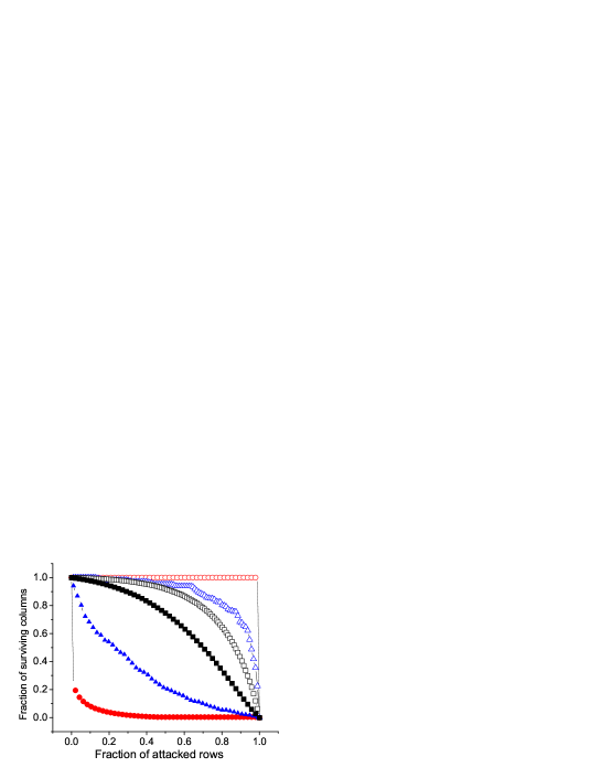
Figure 2: Attack tolerance curves for a matrix of the same size and density of contacts as the real system in [8]. Open symbols correspond to the attack strategy $(-\rightarrow+)$ and solid symbols to the attack strategy $(+\rightarrow-)$. Squares: average ATC over 200 random initial configurations, circles: SNM evolved nested state (average over 200 initial configurations), triangles: real system.

It is interesting to notice that the ATC curves corresponding to the attack strategy $R^{+\rightarrow-}$ change their curvature as the system evolves according to the SNM algorithm. Figure 3 shows three ATCs corresponding to averages over 200 random initial matrices having the same caracteristics as the real system of Clements and Long [8] for three different stages of its evolution, from random to perfect nestedness. Hence, the zero curvature of the ATC may be taken as the indication that the network has lost its random character. In the SNM, the iteration step where the ATC has zero curvature, can be interpreted as an ordering time $t^{*}$. In this exemple this is found at $t^{*}\approx 800$.

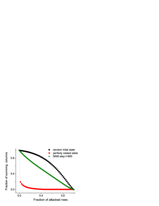
Figure 3: Attack tolerance curves for a matrix of the same size and density of contacts as the real system of Clements and Long [8],under the attack strategy $(+\rightarrow-)$, for three different stages of the evolution of the SNM algorithm. Circles: average ATC over 200 SNM evolved perfectly nested networks , squares: average ATC over 200 random networks, stars: average ATC over 200 SNM evolved networks at an intermediate iteration time of the SNM algorithm, here $t^{*}\approx 800$ steps.

We can then define a nestedness coefficient N as the normalised difference between the robustness coefficients corresponding to the two extreme attack strategies:

$$N=\frac{R^{-\rightarrow+}-R^{+\rightarrow-}}{1-\phi}$$ (1)

Notice that as $1-\phi$ is the area between the two ATC in the case of perfect nestedness, this coefficient is correctly bounded, $N=1$ for perfect nestedness and $N$ decreases for random matrices [13].

In Figure 4 we show the two robustness coefficients and the nesting parameter as a function of the iteration time of the SNM algorithm, starting from random configurations and averaging over 200 samples. The inflexion point of the N(t) is also located at $t^{*}\approx 800$, the time of the SNM evolution which leads to an ATC with zero curvature, indicating again that the ordered phase is setting on.

The analysis we just described assumed that plants (rows) were attacked, leading to a coefficient measuring the robustness of the animals (columns), $N_{c}$. Obviously the same analysis can be done assuming that the animals are attacked, which will lead to a coefficient measuring the robustness of plants, $N_{r}$. In this way, the nestedness of the network is characterised by two parameters $N_{r}$ and $N_{c}$. For real systems [5] it is generally found that the number of animal species is higher that the number of plants species and in that case the SNM model always gives $N_{c}>N_{r}$. This is easy to understand in terms of the SNM algorithm. In fact at a given stage of the SNM iteration, if the update probability is the same for rows and columns, rows are chosen, in average, more often than columns, due to their relative smaller number. Choosing a row means that the update is done over the columns, so at a given iteration time columns are more ordered than rows. This has been checked by simulating a square adjacency matrix having the same total number of sites and the same density as the real system studied in [8], in this case $N_{r}=N_{c}$ for all the SNM evolution. Surprisingly, the same result, $N_{c}>N_{r}$, is found for adjacency matrices corresponding to real networks[8] [11] [12]. This is shown in table 2 where we give the normalized Atmar-Patterson temperature, ${\tilde{T}_{AP}}=T_{AP}/T_{AP,ran}$, with $T_{AP,ran}$, the temperature of the random matrix of the same dimensions and the same density of the considered one. In this way, complete disorder gives ${\tilde{T}_{AP}}=1$

Adjacency Matrix	${\tilde{T}_{AP}}$	$N_{c}$	$N_{r}$
real system Clements	0.16	0.61	0.49
real system Robertson	0.06	0.65	0.58
real system Kato	0.11	0.75	0.57

Table 2: $\tilde{T}_{AP}$ and nestedness coefficient for real matrices [8]  [11] [12].

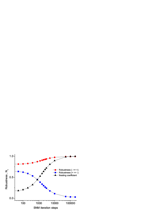
Figure 4: Robustness and Nesting coefficient of the animals (columns) as a function of iteration time of the SNM algorithm, average over 200 initial random networks. Circles correspond to robustness under strategy $R^{-\rightarrow+}$, squares correspond to robustness under strategy $R^{+\rightarrow-}$ and triangles correspond to the nestedness coefficient.

3 Conclusions

We introduce here the nestedness coefficient for plants and animals, as an alternative way to measure the nestedness of the system. Unlike the Atmar and Patterson ”temperature”, which measures an average distance to a supposed perfectly nested state, the nestedness coefficient is operationally defined, based on the robustness of the network. In addition it has the advantage to easily account for the different degrees of order of each guild at any given step of their ordering process.

References

- [1] D.J.Watts and S.H. Strogatz, Nature 393, 440 (1998)
- [2] M.E.J. Newman, S.H. Strogatz and D.J. Watts Phys.Rev. E64, 026128 (2001)
- [3] W. Atmar and B.D. Patterson, Oecologia 96, 373-382 (1993)
- [4] J. Bascompte, P. Jordano, C.J. Meli n, and J.M. Olesen, Proc. Nat. Acad. Sci. USA 100, 9383-9387(2003); P.Jordano, J. Bascompte, J.M. and Olesen, Ecol. Lett. 6, 69-81, (2003); P. Jordano, J. Bascompte, and J.M. Olesen, in Plant-pollinator interactions. From specialization to generalization N. Waser and J. Ollerton, ed., University of Chicago Press. pp 173-199(2006)
- [5] D. Medan, R.P.J. Perazzo, M. Devoto, E. Burgos, M. Zimmermann, H. Ceva and A.M. Delbue, J. of Theor. Biol. 246, 510 (2007)
- [6] E. Burgos, H. Ceva, R.P.J. Perazzo, M. Devoto, D. Medan, M. Zimmermann, and A.M. Delbue, J. of Theor. Biol. 249, 307 (2007)
- [7] Enrique Burgos, Horacio Ceva, Laura Hernández, R.P.J. Perazzo, Mariano Devoto, Diego Medan. arXiv:0805.1407 (2008).
- [8] Clements R. F. , Long F. L., Experimental Pollination. An Outline of the Ecology of Flowers and Insects. Carnegie Institute of Washington. Washington (1923).
- [9] Atmar W. and B. D. Patterson, The nestedness temperature calculator: a visual basic program, including 294 presence-absence matrices AICS Research Inc., University Park, NM and The Field Museum, Chicago, IL (1995).
- [10] Memmott J. , Waser N. M., Price M. V. , Tolerance of pollination networks to species extintions Proc. R. Soc. B 271, 2605-2611 (2004).
- [11] C. Robertson, Science Press Printing Company, Lancaster, Pennsylvania, USA (1929).
- [12] Kato M., Makutani T., Inoue T., Itino T., Insect-flower relationship in the primary beech forest of Ashu, Kyoto: an overview of the flowering phenology and seasonal pattern of insect visits Contr. Biol. Lab. Kyoto Univ. 27, 309-375 (1990).
- [13] In [5] another CPR has been studied (SNM-II), which leads the system to an ordered state having the same amount of contacts in each row and column. This is the antinested state. For this state one finds