Electromagnetic form factor via Bethe-Salpeter amplitude in Minkowski space

Abstract

For a relativistic system of two scalar particles, we find the Bethe-Salpeter amplitude in Minkowski space and use it to compute the electromagnetic form factor. The comparison with Euclidean space calculation shows that the Wick rotation in the form factor integral induces errors which increase with the momentum transfer $Q^{2}$. At JLab domain ($Q^{2}=10\;GeV^{2}/c^{2}$), they are about 30%. Static approximation results in an additional and more significant error. On the contrary, the form factor calculated in light-front dynamics is almost indistinguishable from the Minkowski space one.

1 Introduction

The Bethe-Salpeter (BS) equation [1] provides a field-theoretical framework for a relativistic treatment of few-body systems. It has been extensively studied in the literature (see [2] for a review) and used to obtain relativistic descriptions of two-body bound and scattering states.

BS equation is naturally formulated in the momentum representation. In Minkowski space, for two spinless particles, it reads:

$$\Phi_{M}(k;p) = \frac{i^{2}}{\left[(\frac{p}{2}+k)^{2}-m^{2}+i\epsilon\right]\left[(\frac{p}{2}-k)^{2}-m^{2}+i\epsilon\right]}$$ (1)

$$\times \int\frac{d^{4}k^{\prime}}{(2\pi)^{4}}iK_{M}(k,k^{\prime},p)\Phi_{M}(k^{\prime};p)$$

The interaction kernel $K_{M}$ is given by irreducible Feynman diagrams. Any finite set of them is an approximation of the interaction Lagrangian of the theory under consideration. Most of works were done in the ladder approximation, that is restricting the interaction kernel to its lowest order exchange term. Several researches (in particular [3]) indicate that the higher order kernels, usually not incorporated in the BS equation, give a significant contribution to the two-body binding energy. Studies of these contributions, step by step, in the BS framework, would be of indubitable interest.

Until very recently, the BS equation had been solved only in the Euclidean space, i.e. after performing a Wick rotation [4], in order to remove the singularities due to the free propagators. The validity of Wick rotation has been proved in [4] for the ladder kernel. For higher order kernels (e.g., for the cross box) the possibility of Wick rotation is less clear, since one deals with the ”partially Euclidean” BS amplitude, in which the relative energy $k_{0}=ik_{4}$ is imaginary, whereas the total energy $p_{0}$ remains real. This ”partially Euclidean” transformation is a subtle point to be checked more carefully. We will see below that it is valid also for the cross-ladder kernel. Then the Euclidean BS equation (in the rest frame) provides exactly the same binding energy as the Minkowski one.

If we are interested not only in the binding energy but also in the electromagnetic (EM) form factors, the Euclidean BS amplitude in the rest frame is not enough. On one hand, when computing the integral for the form factor, the rotated contour crosses singularities of the integrand. So, the result is not reduced to the naive replacement $k_{0}=ik_{4}$ which transforms the Minkowski BS amplitude into the Euclidean one. On the other hand, form factor for non-zero momentum transfer involves the BS amplitude for non-zero total momentum $p$. This amplitude can be obtained from the rest frame one by a boost, but the parameters of this boost for real $p$ and imaginary $k_{0}$ are complex. This requires the knowledge of the BS amplitude in the full complex plane. The continuation of the Euclidean amplitude from real axis to the complex plane is numerically very unstable and can hardly be done in practice. Instead of it, the BS amplitude in the complex plane can be found by solving the equation for complex arguments. However, the equation in the complex plane is no longer Euclidean nor Minkowski one and it is actually more complicated than the equation on the real axis. This difficulty is avoided in the so called static approximation [5], which makes use of the Euclidean BS amplitude only but brings an additional error increasing with the momentum transfer.

These problems disappear if one expresses the form factor through the Minkowski BS amplitude. For the ladder kernel, the BS equation in Minkowski space was solved in [6]. For separable interactions, an approach in Minkowski space was developed and applied to the nucleon-nucleon system in [7]. In [8], the effect of the cross-ladder graphs in the BS framework was estimated with the kernel represented through a dispersion relation.

Recently, a new general method to find the Minkowski BS amplitude has been developed [9]. This method is valid for any kernel given by Feynman graphs. In the case of spinless particles, it was tested for the ladder and cross ladder kernels [10].

Having found the Minkowski BS amplitude, we can calculate EM form factor without any approximation. This allows us to check the validity of Wick rotation in the form factor integral, the accuracy of the static approximation and, in addition, to make a comparison with light-front dynamics (LFD) calculations. This is the aim of the present study. A first description of these results, without any derivation, can be found in [11].

This article is organized as follows. In sect. 2 we briefly describe the method [9] for solving the BS equation in Minkowski space and give new validity tests. In sect. 3 the Minkowski space calculation of form factor is presented. In sect. 4 the analogous Euclidean space computation is carried out, including its static approximation. In sect. 5 the form factor in the LFD framework is calculated. The comparison of numerical calculations performed in the different approaches considered in this work is given in sect. 6. Finally, some concluding remarks are presented in sect. 7.

2 The method

According to [9, 10], the Minkowski space BS amplitude is found in terms of the Nakanishi integral representation [2, 12]:

$$\Phi_{M}(k;p) = -{i\over\sqrt{4\pi}}\int_{-1}^{1}dz\int_{0}^{\infty}d\gamma$$ (2)

$$\times \frac{g(\gamma,z)}{\left[\gamma+m^{2}-\frac{1}{4}M^{2}-k^{2}-p\cdot k\;z-i\epsilon\right]^{3}}.$$

The weight function $g(\gamma,z)$ itself is not singular, whereas the singularities of the BS amplitude are fully reproduced by this integral. For example, if we set $-{i\over\sqrt{4\pi}}g(\gamma,z)=1$ and calculate the integral, we find

$$\Phi_{M}(k;p)=\frac{i^{2}}{\left[(\frac{p}{2}+k)^{2}-m^{2}+i\epsilon\right]\left[(\frac{p}{2}-k)^{2}-m^{2}+i\epsilon\right]},$$

i.e. just the product of two free propagators in (1). $\Phi_{M}$ in the form (2) is substituted into the BS equation (1) and after some mathematical transformations [9], one obtains the following integral equation for $g(\gamma,z)$:

$$\int_{0}^{\infty}\frac{g(\gamma^{\prime},z)d\gamma^{\prime}}{\Bigl{[}\gamma^{\prime}+\gamma+z^{2}m^{2}+(1-z^{2})\kappa^{2}\Bigr{]}^{2}}=$$

$$\int_{0}^{\infty}d\gamma^{\prime}\int_{-1}^{1}dz^{\prime}\;V(\gamma,z;\gamma^{\prime},z^{\prime})g(\gamma^{\prime},z^{\prime}),$$ (3)

where $\kappa^{2}=m^{2}-\frac{1}{4}M^{2}$ and $V$ is calculated in terms of kernel $K_{M}$ [9]. A remarkable point is that equation (2) is strictly equivalent to the original BS equation (1) and does not contain any singularity neither in $g(\gamma,z)$ nor in $V$. Once $g(\gamma,z)$ is found by solving (2), the Minkowski BS amplitude is obtained by expression (2).

Equation for the Euclidean BS amplitude is obtained from the Minkowski one (1) in the center of mass frame $\vec{p}=0$, by the Wick rotation and substitution $k_{0}=ik_{4}$

$$\left[\left(k_{4}^{2}+k^{2}+m^{2}-\frac{M^{2}}{4}\right)^{2}+M^{2}k_{4}^{2}\right]\Phi_{E}(k_{4},\vec{k})=$$

$$\int\frac{dk^{\prime}_{4}d^{3}k^{\prime}}{(2\pi)^{4}}K_{E}(k_{4},\vec{k};k^{\prime}_{4},\vec{k^{\prime}})\Phi_{E}(k^{\prime}_{4},\vec{k^{\prime}}),$$ (4)

where

$$\Phi_{E}(k_{4},\vec{k})=\Phi_{M}(ik_{4},\vec{k};M,\vec{p}=0)$$ (5)

and $K_{E}(k_{4},\vec{k};k^{\prime}_{4},\vec{k^{\prime}})=K_{M}(ik_{4},\vec{k};ik^{\prime}_{4},\vec{k^{\prime}};M,\vec{p}=0).$ By the method developed in [9] we can restore the Euclidean BS amplitude, i.e., find the solution of (4), by setting in (2) $k_{0}=ik_{4}$ and $\vec{p}=0$.

All three equations (1), (2) and (4) are equivalent to each other in the sense that they give the same $M^{2}$. In [9] the equivalence of (2) to the initial BS equation (1) has been checked numerically for the ladder kernel. It was found that the binding energies $B=2m-M$ coincide with high precision.

For more complete checks, we present here two additional tests. In the first one, still for the ladder kernel, we compare the Euclidean BS amplitudes obtained by inserting the solution of (2) into (2), where $k=(ik_{4},\vec{k})$, $p=(M,\vec{0})$, with the one found by directly solving (4). These amplitudes are plotted in fig. 1 (top). They coincide at a level better than 0.2% on the whole range of $(|\vec{k}|,k_{4})$ considered and are indistinguishable from each other in the graph. On the contrary, the Euclidean BS amplitude strongly differs from the initial Minkowski one, shown at the bottom part of fig. 1. It is worth reminding that so different amplitudes (compare top and bottom of fig. 1) correspond to one and the same mass $M$.

    

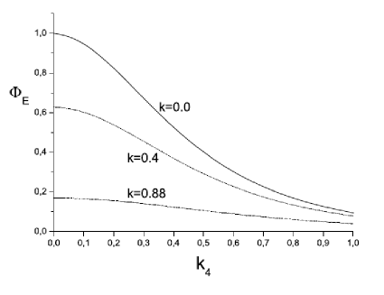
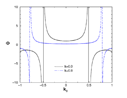
Figure 1: Top: The Euclidean BS amplitude (for ladder kernel) obtained by (2) with $k_{0}=ik_{4}$, for different values of $k$. Or (indistinguishable) the one calculated by direct resolution of BS equation in Euclidean space (4). The exchange mass is $\mu=0.5$.
Bottom: The corresponding amplitude in Minkowski space, obtained in [9, 13]. We use the units $m=1$.

[!ht]

Table 1: Coupling constant $\alpha$ for given values of the binding energy $B$ calculated by the eq. (2) and by the Euclidean BS equation (4) for the ladder +cross-ladder (L+CL) kernel. The exchanged mass: $\mu=0.5$.

$B$	0.01	0.05	0.10	0.20	0.50	1.00
$\alpha$, eq. (2)	1.206	1.607	1.930	2.416	3.446	4.549
$\alpha$, Euclid, eq. (4)	1.205	1.608	1.930	2.417	3.448	4.551

Figure 2: Feynman cross ladder graph.

The second test incorporates, in addition, the cross ladder kernel displayed in fig. 2. For a massive exchange and a wide range of binding energies $B$, we carried out precise calculations (accuracy better than 0.1%) of the corresponding coupling constants $\alpha=g^{2}/(16\pi m^{2})$ both by equation (2) and by Euclidean equation (4) (here $g$ is the coupling constant in the interaction Hamiltonian). The results are displayed in the table 1 in units of $m$. Their coincidence demonstrates the validity of both calculations – in Minkowski space by the method [9] and in Euclidean one.

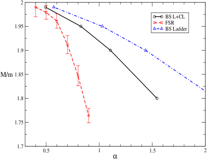
Figure 3: Ground state mass $M$ obtained by the Bethe-Salpeter ladder and cross-ladder kernel, compared with the Feynman-Schwinger representation results for an exchanged mass $\mu=0.15$.

The ladder or ladder +cross-ladder kernels are good enough to check the applicability of the method [9]. We would like to emphasize, however, that both kernels give a rather crude approximation of the full interaction. Figure 3 shows the ground state mass $M$ obtained, for $\mu=0.15$, by the BS ladder and ladder +cross-ladder kernels together with Feynman-Schwinger representation results [3]. The latter incorporates all the higher order cross box contributions in the kernel, but not the self energy. Even at low binding energies, the ladder and cross-ladder results differ by at least 20%, this difference reaching more than a factor 2 around $B/m=1$. On the other hand, the results obtained by Feynman-Schwinger representation departs strongly from the BS(L+CL) as soon as $B$ is bigger than $0.05\,m$. The cross-ladder kernel thus gives a non negligible contribution to the total mass of the system in the right direction, but a larger contribution remains to be included, due to the higher order terms. Notice however that the underlying field theory with cubic boson-boson interaction is unbounded from below [14]. This instability (for the interaction $g\phi\chi^{2}$) appears when infinite number of the $\chi^{2}$ loops in the field $\phi$ self energy is included [15].

3 EM form factor via Minkowski BS amplitude

Figure 4: Feynman diagram for the EM form factor.

The electromagnetic vertex is shown in Fig. 4. We suppose that one of the particles is charged. By applying the Feynman rules to this graph, we get:

$$(p+p^{\prime})^{\nu}F_{M}(Q^{2})=i\int\frac{d^{4}k}{(2\pi)^{4}}\,\frac{(p+p^{\prime}-2k)^{\nu}}{(k^{2}-m^{2}+i\epsilon)}$$

$$\times\,\frac{\Gamma\left(\frac{1}{2}p-k,p\right)\Gamma\left(\frac{1}{2}p^{\prime}-k,p^{\prime}\right)}{[(p-k)^{2}-m^{2}+i\epsilon][(p^{\prime}-k)^{2}-m^{2}+i\epsilon]},$$ (6)

where $\Gamma(k,p)$ is the vertex function, related to the BS amplitude by:

$$\Phi_{M}(k;p)=\frac{\Gamma(k,p)}{\left[(\frac{p}{2}+k)^{2}-m^{2}+i\epsilon\right]\left[(\frac{p}{2}-k)^{2}-m^{2}+i\epsilon\right]}.$$ (7)

Therefore the electromagnetic vertex is expressed in terms of the BS amplitude by the formula:

$$(p+p^{\prime})^{\nu}F_{M}(Q^{2})=i\int\frac{d^{4}k}{(2\pi)^{4}}\,(p+p^{\prime}-2k)^{\nu}$$

$$\times\;(k^{2}-m^{2})\,\Phi_{M}\left(\frac{1}{2}p-k;p\right)\Phi_{M}\left(\frac{1}{2}p^{\prime}-k;p^{\prime}\right).$$ (8)

We multiply both sides of (3) by $(p+p^{\prime})_{\mu}$ and substitute in its r.h.s. the BS amplitude in terms of the integral (2). So, the form factor is given by:

$$(p+p^{\prime})^{2}F_{M}(Q^{2})=\int\frac{id^{4}k}{2(2\pi)^{5}}\,d\gamma dz\,d\gamma^{\prime}dz^{\prime}\,g(\gamma,z)g(\gamma^{\prime},z^{\prime})$$

$$\times\frac{\left[(p+p^{\prime})^{2}-2k\cdot(p+p^{\prime})\right]\,(m^{2}-k^{2})}{\left[\gamma+m^{2}-\frac{1}{4}M^{2}-(\frac{1}{2}p-k)^{2}-p\cdot(\frac{1}{2}p-k)\;z-i\epsilon\right]^{3}}$$

$$\times\frac{1}{\left[\gamma^{\prime}+m^{2}-\frac{1}{4}M^{2}-(\frac{1}{2}p^{\prime}-k)^{2}-p^{\prime}\cdot(\frac{1}{2}p^{\prime}-k)\;z^{\prime}-i\epsilon\right]^{3}}$$

To compute this integral, we use the Feynman parametrization:

$$\frac{1}{a^{3}b^{3}}=\int_{0}^{1}\frac{30u^{2}(1-u)^{2}du}{\Bigl{(}au+b(1-u)\Bigr{)}^{6}}$$

and then shift the integration variable:

$$k=k_{1}+\frac{1}{2}(1+z)u\;p+\frac{1}{2}(1+z^{\prime})(1-u)\;p^{\prime}.$$ (9)

Then the integral over $d^{4}k_{1}$ has the form

$$\int\frac{\cdots d^{4}k_{1}}{(k_{1}^{2}-c+i\epsilon)^{6}},$$ (10)

where $c$ does not depend on $k_{1}$. Though the calculation of this integral by Wick rotation is standard, we explain it here in more detail, to emphasize the difference with the calculation performed using Euclidean BS amplitude, where the Wick rotation cannot be done (see sect. 4 below). The integrand in (10) does not contain linear terms in $k_{10}$, but only a constant and a quadratic term. It has four poles at the values $k_{10}=\pm\sqrt{c^{2}+\vec{k}^{2}_{1}}\mp i\epsilon$. Their positions do not prevent from the counter-clock-wise rotation of the integration contour. Therefore, substituting here $k_{10}=ik_{4}$, we get, for the constant term in $k_{10}$, the following relations:

$$\int\frac{d^{4}k_{1}}{(k_{1}^{2}-c+i\epsilon)^{6}}=\int\frac{dk_{10}d^{3}k_{1}}{(k^{2}_{10}-\vec{k}_{1}^{2}-c+i\epsilon)^{6}}$$ (11)

$$= \int\frac{idk_{4}d^{3}k_{1}}{(k^{2}_{4}+\vec{k}_{1}^{2}+c)^{6}}=\int_{0}^{\infty}\frac{i2\pi^{2}k^{3}dk}{(k^{2}+c)^{6}}=\frac{2i\pi^{2}}{40c^{4}}.$$

Calculating similarly the integral for the quadratic term

$$\int\frac{k_{1}^{2}\;d^{4}k_{1}}{(k_{1}^{2}-c+i\epsilon)^{6}}=-\frac{2i\pi^{2}}{60c^{3}},$$ (12)

we find the following formula, which is exact for a given $g(\gamma,z)$:

$$F_{M}(Q^{2}) = \frac{1}{2^{7}\pi^{3}N_{M}}\int_{0}^{\infty}d\gamma\int_{-1}^{1}dz\,g(\gamma,z)$$

$$\times \int_{0}^{\infty}d\gamma^{\prime}\int_{-1}^{1}dz^{\prime}\,g(\gamma^{\prime},z^{\prime})\int_{0}^{1}du\,u^{2}(1-u)^{2}\frac{f_{num}}{f^{4}_{den}}$$

with

$$f_{num} = (6\xi-5)m^{2}+[\gamma^{\prime}(1-u)+\gamma u](3\xi-2)$$

$$+ 2M^{2}\xi(1-\xi)+\frac{1}{4}Q^{2}(1-u)u(1+z)(1+z^{\prime})$$

$$f_{den} = m^{2}+\gamma^{\prime}(1-u)+\gamma u-M^{2}(1-\xi)\xi$$

$$+ \frac{1}{4}Q^{2}(1-u)u(1+z)(1+z^{\prime}),$$

where $Q^{2}=-(p-p^{\prime})^{2}>0$. To simplify the formula, we use the notation:

$$\xi=\frac{1}{2}(1+z)u+\frac{1}{2}(1+z^{\prime})(1-u).$$

We have also introduced in (3) the normalization factor $N_{M}$ which is found from the condition $F_{M}(0)=1$.

4 EM form factor via Euclidean BS amplitude

Form factor (3) was calculated using a well justified Wick rotation in the variable $k_{10}$, defined by (9). As explained in sect. 2, the Euclidean BS amplitude in the rest frame $\Phi_{E}(k_{4},\vec{k})$ is obtained from the Minkowski one (see eq. (5)) by Wick rotation in the variable $k_{0}$. To express the form factor through $\Phi_{E}(k_{4},\vec{k})$, one should make the Wick rotation, in the variable $k_{0}$, in integral (3) (for the moment, we ignore the fact that the BS amplitude in (3) is not in the rest frame; we will come back to this point later). We will show that, in contrast to integrals (11) and (12), the Wick rotation in (3) cannot be done without crossing singularities. Therefore the form factor cannot be expressed through the Euclidean BS amplitude exactly.

It is enough to illustrate this statement in the simplest case, with $\Gamma(k,p)=1$ and $p^{\prime}=p=(M,\vec{0})$, i.e. $Q^{2}=0$ and $\nu=0$. Integral (3) then turns into:

$$I=\int\frac{d^{4}k}{(2\pi)^{4}}\,\frac{2i(M-k_{0})}{(k^{2}-m^{2}+i\epsilon)[(p-k)^{2}-m^{2}+i\epsilon]^{2}}.$$

The first propagator has poles at $k_{0}=\pm\sqrt{m^{2}+\vec{k}^{2}}\mp i\epsilon$ and this does not create any problem, whereas the second factor has poles at:

$$k_{0}=M\pm\sqrt{m^{2}+\vec{k}^{2}}\mp i\epsilon$$

If $\vec{k}^{2}<M^{2}-m^{2}$, both poles are in the r.h.s. half plane and the pole at $k_{0}=M-\sqrt{m^{2}+\vec{k}^{2}}+i\epsilon$ prevents from the Wick rotation. The exact result for the form factor should incorporate the residue in this pole and therefore it is not reduced to the integral obtained from (3) by the naive replacement $k_{0}=ik_{4}$. If the residue is omitted (or, in realistic case, if the contributions of other possible singularities of $\Gamma(k,p)$ crossed by the rotated contour are omitted) the result is approximate. In practice, taking into account the contributions of these unavoidable singularities is impossible and, hence, the form factor calculated through the Euclidean BS amplitude is always approximate.

Shifting the variable $k_{0}$ (for example, $k_{0}\to-k_{0}+\frac{1}{2}p_{0}$, to transform the argument $\frac{1}{2}p_{0}-k_{0}$ of the BS amplitude in (3) into $k_{0}$) does not help. The situation remains the same for non-trivial $\Gamma(k,p)$ and for non-zero $Q^{2}$.

In addition, there is another reason which does not allow to express the form factor via Euclidean BS amplitude. The latter is determined by eq. (4) in the rest frame $\vec{p}=0$ and it is related to the Minkowski one by eq. (5). However, the form factor is expressed through the BS amplitude with non-zero total momenta $\vec{p}$ and $\vec{p^{\prime}}$ which due to scattering are different in initial and final states. Hence, after Wick rotation, we need to know

$$\Phi_{E}^{boost}(k_{4},\vec{k};p)=\Phi_{M}(ik_{4},\vec{k};p).$$ (14)

which differs from the Euclidean BS amplitude $\Phi_{E}(k_{4},\vec{k})$ in eq. (5), by non-zero value of $\vec{p}$. They are identical only at $\vec{p}=0$. The boosted amplitude $\Phi_{E}^{boost}(k_{4},\vec{k};p)$ can be expressed through $\Phi_{E}(k_{4},\vec{k})$, but only for complex values of its arguments $k_{4},|\vec{k}|$.

Indeed, the Minkowski amplitude $\Phi_{M}(k_{0},\vec{k};p)$ in r.h.s. of (14), for real $k_{0}$ and for non-zero $\vec{p}$, can be found from the rest frame amplitude by a boost. Namely, we can take the BS amplitude $\Phi_{M}(k_{0},|\vec{k}|;M,\vec{p}=0)$ in the rest frame and substitute

$$k_{0} \to k^{\prime}_{0}=\frac{1}{M}(p_{0}k_{0}-\vec{p}\cdot\vec{k}),$$

$$|\vec{k}| \to |\vec{k^{\prime}}|=\sqrt{{k^{\prime}}^{2}_{0}-k_{0}^{2}+\vec{k}^{2}}.$$

That is:

$$\Phi_{M}(k_{0},\vec{k};p)=\Phi_{M}(k^{\prime}_{0},|\vec{k^{\prime}}|;M,\vec{p}=0).$$

To get the Euclidean amplitude, we replace here $k_{0}=ik_{4}$, $k^{\prime}_{0}=ik^{\prime}_{4}$, substitute the result in (14) and use the definition (5). Then the relation (14) has the form:

$$\Phi^{boost}_{E}(k_{4},\vec{k};p)=\Phi_{E}(k^{\prime}_{4},k^{\prime})$$

where $\Phi_{E}(k^{\prime}_{4},k^{\prime})$ is the Euclidean BS amplitude in the rest frame, depending however on the complex arguments:

$$k^{\prime}_{4}=\frac{1}{M}(p_{0}k_{4}+i\vec{p}\cdot\vec{k}),\quad k^{\prime}=\sqrt{k_{4}^{2}+\vec{k}^{2}-{k^{\prime}_{4}}^{2}}.$$ (15)

This requires the knowledge of the Euclidean BS amplitude $\Phi_{E}(k^{\prime}_{4},k^{\prime})$ in the full complex plane. Alternatively, one can solve the Euclidean BS equation for non-zero $\vec{p}$ (for real arguments) and obtain $\Phi^{boost}_{E}(k_{4},\vec{k};p)$ directly. These solutions for quark systems were found numerically in [16]. In sect. 4.1 we will find them, making the substitution $k_{0}=ik_{4}$ in (2).

In view of these two facts, the EM form factor can be expressed through the Euclidean BS amplitude only approximately. Below, we will study the accuracy of the following two approximations.

(i) Naive Euclidean form factor. In this case, the form factor is found by the naive substitution $k_{0}=ik_{4}$ in the Minkowski expression (3). This corresponds to an approximate Wick rotation which disregards singularities. However, the BS amplitude in the complex plane $\Phi_{E}(k^{\prime}_{4},k^{\prime})$ can be found exactly, by substituting in eq. (2) the complex values (15) of boosted arguments.

(ii) Naive Euclidean form factor in the static approximation. In this case, the form factor is still found by the substitution $k_{0}=ik_{4}$ in (3). In addition, the boosted amplitude $\Phi^{boost}_{E}(k_{4},\vec{k};p)=\Phi_{E}(k^{\prime}_{4},k^{\prime})$ is approximately replaced by the amplitude at rest $\Phi^{boost}_{E}(k_{4},\vec{k};M,\vec{p}=0)=\Phi_{E}(k_{4},k)$. Due to that, the form factor is expressed through the Euclidean BS amplitude with real arguments.

4.1 Naive Euclidean form factor

In order to obtain the naive Euclidean form factor, we start with the Minkowski space formula (3). We use the Breit frame defined as:

$$\vec{p^{\prime}}=-\vec{p},\quad p_{0}^{\prime}=p_{0}=\sqrt{M^{2}+p^{2}},\quad Q^{2}=4p^{2}.$$

and shift the integration variable: $k_{0}\to-k_{0}+\frac{1}{2}p_{0}.$ The spatial components of eq. (3) in the Breit frame are trivially satisfied (0=0). Taking the time-component, we get:

$$2p_{0}F_{M}(Q^{2})=\int\frac{id^{4}k}{(2\pi)^{4}}\left[\left(\frac{p_{0}}{2}-k_{0}\right)^{2}-\vec{k}^{2}-m^{2}\right]$$

$$\times (p_{0}+2k_{0})\,\Phi_{M}\left(k_{0},\frac{1}{2}\vec{p}-\vec{k};p\right)\Phi_{M}\left(k_{0},-\frac{1}{2}\vec{p}-\vec{k};p^{\prime}\right)$$

We simply replace: $k_{0}=ik_{4}$ with real $k_{4}$, that is, we neglect the contributions of singularities crossed by the rotated contour, and we obtain:

$$F^{naive}_{E}(Q^{2})=\int\frac{dk_{4}d^{3}k}{2p_{0}(2\pi)^{4}}\;(p_{0}+2ik_{4})$$

$$\phantom{F^{naive}_{E}(Q^{2})}\times\left[m^{2}+\vec{k}^{2}-\left(\frac{p_{0}}{2}-ik_{4}\right)^{2}\right]$$

$$\times \Phi^{boost}_{E}\left(k_{4},\frac{1}{2}\vec{p}-\vec{k};p\right)\Phi^{boost}_{E}\left(k_{4},-\frac{1}{2}\vec{p}-\vec{k};p^{\prime}\right)$$

where $\Phi^{boost}_{E}(k_{4},\vec{k};p)$ is defined in (14). Substituting in r.h.s. of (14) the BS amplitude from eq. (2), one gets:

$$\Phi^{boost}_{E}(k_{4},\vec{k},p)=-{i\over\sqrt{4\pi}}\int_{-1}^{1}dz\int_{0}^{\infty}d\gamma$$

$$\times \frac{g(\gamma,z)}{\left[\gamma+m^{2}-\frac{1}{4}M^{2}+k_{4}^{2}+\vec{k}^{2}-(ip_{0}k_{4}-\vec{p}\cdot\vec{k})\;z-i\epsilon\right]^{3}}$$

After substituting (4.1) in (4.1), the form factor
$F^{naive}_{E}(Q^{2})$ is expressed as:

$$F^{naive}_{E}(Q^{2}) = \frac{1}{N^{naive}_{E}}\int_{0}^{\infty}d\gamma^{\prime}\int_{-1}^{1}dz^{\prime}\;g(\gamma^{\prime},z^{\prime})\int_{0}^{\infty}d\gamma$$

$$\times \int_{-1}^{1}dz\;g(\gamma,z)\int_{0}^{\infty}dk_{4}\int_{0}^{\infty}d^{3}k\;f(k_{4},\vec{k},\vec{p}),$$

where

$$f(k_{4},\vec{k},\vec{p})=-\frac{1}{2^{6}\pi^{5}p_{0}}\mbox{Re}[U(k_{4},\vec{k},\vec{p})]$$

$$U(k_{4},\vec{k},\vec{p})=\frac{\left[k^{2}+m^{2}+(k_{4}+\frac{1}{2}ip_{0})^{2}\right](2ik_{4}+p_{0})}{D^{3}{D^{\prime}}^{3}}$$

with

$$D = A-\vec{p}\cdot\vec{k}\,(1+z)+\frac{1}{4}(1+2z)\vec{p}^{2}-ik_{4}p_{0}z-i\epsilon,$$

$$A = \gamma+m^{2}-\frac{1}{4}M^{2}+k_{4}^{2}+\vec{k}^{2}$$ (20)

and $p_{0}=\sqrt{M^{2}+\vec{p}^{2}}$. $D^{\prime},A^{\prime}$ are obtained from $D,A$ by the replacements $\gamma\to\gamma^{\prime}$, $z\to z^{\prime}$. The normalization factor $N^{naive}_{E}$ is again found from the condition $F^{naive}_{E}(0)=1$.

Like Minkowski space form factor (3), the form factor (4.1) is expressed through the function $g(\gamma,z)$, satisfying (2), but differs from (3) by neglecting singularities crossed when performing the Wick rotation. Their comparison in sect. 6 will show the error induced by this approximation.

Note that the denominators $D$ and $D^{\prime}$, for some momentum transfer $Q^{2}$ and the integration variables, may be zero. For example, for $\gamma=0$, $z=1$, $k_{4}=0$ we get:

$$D=m^{2}-\frac{1}{4}M^{2}-\frac{1}{16}Q^{2}+(\vec{p}-\vec{k})^{2}-i\epsilon$$

(we used that $Q^{2}=4p^{2}$). Since $m^{2}-\frac{1}{4}M^{2}$ is positive, $D$ is always positive too if

$$Q^{2}<4(4m^{2}-M^{2}).$$ (21)

If $Q^{2}>4(4m^{2}-M^{2})$, $D$ crosses zero for some particular values of $\vec{p}$ and $\vec{k}$. This singularity is, of course, integrable (the form factor is always finite), but it is a source of numerical instability.

4.2 Naive Euclidean form factor in the static approximation

As explained in the previous section, the form factor (4.1) is expressed through the BS amplitude $\Phi^{boost}_{E}(k_{4},\vec{k},p)$ which for $\vec{p}\neq 0$, is in its turn expressed through the Euclidean BS amplitude in the complex plane. If we replace the latter by the Euclidean BS amplitude in the rest frame $\Phi_{E}(k_{4},\vec{k})=\Phi^{boost}_{E}(k_{4},\vec{k};M,\vec{p}=0)$, satisfying equation (4), we obtain the form factor in the so called static approximation, which reads:

$$F^{stat}_{E}(Q^{2}) = \frac{1}{N_{E}}\int\frac{dk_{4}d^{3}k}{2(2\pi)^{4}}\left(m^{2}+\vec{k}^{2}-k_{4}^{2}-\frac{1}{4}p_{0}^{2}\right)$$ (22)

$$\times \Phi_{E}\left(k_{4},\frac{1}{2}\vec{p}-\vec{k}\right)\Phi_{E}\left(k_{4},-\frac{1}{2}\vec{p}-\vec{k}\right)$$

Notice that no approximation in the kinematical factor is done, though we omit the odd degrees of $k_{4}$, since after integration over $dk_{4}$ they give zero.

As mentioned, $\Phi_{E}(k_{4},\vec{k})$ can be found from equation (4). If $g(\gamma,z)$ is known, $\Phi_{E}(k_{4},\vec{k})$ can be alternatively obtained by equation (4.1) at $\vec{p}=0$. In this case, the integral (4.1) is reduced to:

$$\Phi_{E}\left(k_{4},\vec{k}\right)=-i\int_{0}^{1}dz\int_{0}^{\infty}d\gamma\frac{g(\gamma,z)2A(A^{2}-3k_{4}^{2}M^{2}z^{2})}{\sqrt{4\pi}(A^{2}+k_{4}^{2}M^{2}z^{2})^{3}},$$

where $A$ is defined in (4.1).

5 EM form factor via light-front wave function

Knowing the Minkowski BS amplitude, we can find the light-front wave function [17]:

$$\psi(\vec{k}_{\perp},x)=\frac{(\omega\cdot k_{1})(\omega\cdot k_{2})}{\pi(\omega\cdot p)}\int_{-\infty}^{+\infty}\Phi_{M}(k+\beta\omega,p)d\beta.$$ (23)

Here $\omega$ is a four-vector with $\omega^{2}=0$, determining the orientation of the light-front plane. The perp-components of vectors, which appear below, are defined relative to the direction $\vec{\omega}$. Relation (23) is independent of any model. Substituting (2) into (23), we find the two-body light-front wave function:

$$\psi(\vec{k}_{\perp},x)=\frac{1}{\sqrt{4\pi}}\int_{0}^{\infty}\frac{x(1-x)g(\gamma,1-2x)d\gamma}{\Bigl{(}\gamma+\vec{k}_{\perp}^{2}+m^{2}-x(1-x)M^{2}\Bigr{)}^{2}}\ .$$ (24)

The form factor is expressed through this wave function as (see e.g. [17]):

$$F_{LFD}(Q^{2})=\frac{1}{(2\pi)^{3}}\int\psi(\vec{k}_{\perp},x)\psi(\vec{k}_{\perp}-x\vec{Q}_{\perp},x)\frac{d^{2}k_{\perp}dx}{2x(1-x)},$$ (25)

where ${\vec{Q}}_{\perp}^{2}=Q^{2}$. Substituting in (25) the wave function $\psi(\vec{k}_{\perp},x)$ determined by eq. (24) and using the formula

$$\frac{1}{a^{2}b^{2}}=\int_{0}^{1}\frac{6u(1-u)du}{\Bigl{(}au+b(1-u)\Bigr{)}^{4}},$$

we can easily integrate over $\vec{k}_{\perp}$ and write the form factor as:

$$F_{LFD}(Q^{2})=\frac{1}{2^{5}\pi^{3}N_{LFD}}\int_{0}^{\infty}d\gamma^{\prime}\int_{0}^{\infty}d\gamma\int_{0}^{1}dx\int_{0}^{1}du$$

$$\times\frac{x(1-x)\,u(1-u)\,g(\gamma,2x-1)g(\gamma^{\prime},2x-1)}{\left[u\gamma+(1-u)\gamma^{\prime}+u(1-u)x^{2}Q^{2}+m^{2}-x(1-x)M^{2}\right]^{3}}.$$

(26)

6 Numerical results

All the calculations given below have been done with the BS amplitude found for the ladder+cross ladder kernel. The constituent mass $m=1$, the exchange mass $\mu=0.5$ and the coupling constant $\alpha$ has been adjusted to provide the binding energy $B=1$.

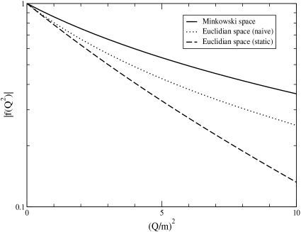
Figure 5: Solid curve: form factor via Minkowski BS amplitude. Dotted curve: form factor, after Wick rotation, with boosted Euclidean BS amplitude. Dashed curve: form factor in static approximation.

For $Q^{2}\leq 10\,m^{2}$ (”JLab domain”), the naive Euclidean form factor and its static approximation are compared with the Minkowski one in fig. 5. Solid curve is the Minkowski space calculation, eq. (3). Dotted curve represents the naive Euclidean form factor calculated with boosted Euclidean BS amplitude by eq. (4.1). Dashed curve denotes the form factor in the static approximation, eq. (22). The difference between solid and dotted curves shows that indeed some singularities are missed and, therefore, the Wick rotation in the variable $k_{0}$ results in an inaccuracy. The static approximation (dashed curve) generates an additional error, increasing with $Q^{2}$.

Binding energy $B=1$ corresponds to $M=m$. In this case, the condition (21) is violated if $Q^{2}>12\,m^{2}$. Indeed, our numerical calculation became unstable if $Q^{2}$ crosses $\approx 12\,m^{2}$. That is why the domain of $Q^{2}$ in fig. 5 does not exceeds $10\,m^{2}$. This difficulty is absent in the static approximation.

Figure 6 shows the comparison between form factors calculated in Minkowski space (solid) and in the static approximation (dashed) in a wider domain of momentum transfer. For high $Q^{2}$, the static form factor is smaller than the Minkowski one by at least a factor 10. A zero in the static form factor at $Q^{2}\approx 38\,m^{2}$ is an artefact of the static approximation, since it is absent in the exact (Minkowski space) form factor.

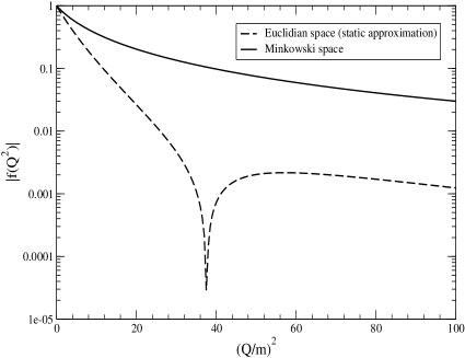
Figure 6: Form factor via Minkowski BS amplitude (solid curve) and in static approximation (dashed).

Figure 7 shows the comparison between the form factors calculated in Minkowski space (solid curve, the same as in fig. 6) and in LFD, eq. (26) (dot-dashed curve). The LFD form factor is almost indistinguishable from the Minkowski one in all domain of momentum transfer.

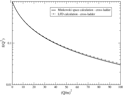
Figure 7: Form factor via Minkowski BS amplitude (solid curve, the same as in fig. 6) and in LFD (dot-dashed curve).

7 Conclusion

We have applied the solution of the BS equation in Minkowski space, found by the method developed in [9, 10], to calculate the EM form factor and to evaluate the inaccuracy of different approximations available in the literature. This method gives the BS amplitudes both in Minkowski and Euclidean spaces as well as in the full complex plane. We presented two additional validity tests of this method and demonstrated that it gives the same Euclidean BS amplitude as the one found by directly solving equation (4). For the ladder and ladder +cross ladder kernel, it gives the same binding energy.

We calculated the electromagnetic form factor exactly, via Minkowski space BS amplitude. To express it through the Euclidean solution, one should carry out the Wick rotation, which, however, requires to incorporate the contributions of the singularities, crossed by the rotating integration contour. In the naive Euclidean form factor, they are omitted. In addition, after Wick rotation, the Euclidean BS amplitude in a moving reference frame (i.e., boosted BS amplitude) is expressed through the rest frame one, depending on complex arguments. By our method [9], we find the BS amplitude in complex plane and analyze the error resulting from naive Wick rotation. The error increases with momentum transfer and at $Q^{2}\approx 10\,m^{2}$ (”JLab domain”) it is about 30%. In the static approximation, the error becomes larger, so that at $Q^{2}\approx 10\,m^{2}$ the Minkowski- and static-approximation form factors differ by one order of magnitude. The three form factors – the exact one from Minkowski BS amplitude, the Euclidean boosted one and in static approximation – are found to be close to each other (within a few per cents) only at relatively small momentum transfer $Q^{2}\leq m^{2}$.

The form factors calculated using the Minkowski space BS amplitude and the light-front wave function coincide with each other with very high accuracy. They are almost indistinguishable.

Note that, in contrast to the Minkowski space BS amplitude, the light-front wave function is not singular and can be found directly, from the corresponding 3D equation [17], without using any BS formalism and eq. (24). This advantage, together with accurate result for the form factor (see figure 7), is one of the reasons which makes the application of the light-front approach to the EM form factor rather attractive.

The system of spinless particles considered in this work, provides a simple model giving a lower limit of different approximations accuracy to the form factor. One can expect that incorporating spin, these errors would increase.

References

• [1] E.E. Salpeter, H.A. Bethe, Phys. Rev. 84, 1232 (1951).
• [2] N. Nakanishi, Prog. Theor. Phys. Suppl. 43, 1 (1969); 95, 1 (1988).
• [3] T. Nieuwenhuis and J.A. Tjon, Phys. Rev. Lett. 77, 814 (1996).
• [4] G.C. Wick, Phys. Rev 96, 1124 (1954).
• [5] M.J. Zuilhof and J.A. Tjon, Phys. Rev. 22, 2369 (1980).
• [6] K. Kusaka, A.G. Williams, Phys. Rev. D 51, 7026 (1995); K. Kusaka, K. Simpson, A.G. Williams, Phys. Rev. D 56, 5071 (1997).
• [7] S.G. Bondarenko, V.V. Burov, A.M. Molochkov, G.I. Smirnov and H. Toki, Prog. in Part. and Nucl. Phys., 48, 449 (2002).
• [8] A. Amghar, B. Desplanques and L. Theusl, Nucl. Phys. A 694, 439 (2001).
• [9] V.A. Karmanov and J. Carbonell, Eur. Phys. J. A 27, 1 (2006) [arXiv:hep-th/0505261].
• [10] J. Carbonell and V.A. Karmanov, Eur. Phys. J. A 27, 11 (2006) [arXiv:hep-th/0505262].
• [11] V.A. Karmanov, J. Carbonell, M. Mangin-Brinet, Nucl. Phys. A 790, 598c (2007) [arXiv:hep-th/0610158]; V.A. Karmanov, J. Carbonell, M. Mangin-Brinet, Proc. of the 20th Int. Conf. on Few-Body Problems in Physics (FB20), Pisa, Italy, September 10-14, 2007, to be published in ”Few-Body Systems” [arXiv:0712.0971].
• [12] N. Nakanishi, Phys. Rev. 130, 1230 (1963); Graph Theory and Feynman Integrals, (Gordon and Breach, New-York, 1971).
• [13] V.A. Karmanov and J. Carbonell, Nucl. Phys. B (Proc.Suppl.) 161, 123 (2006) [arXiv:nucl-th/0510051].
• [14] G. Baym, Phys. Rev. 117, 886 (1960).
• [15] F. Gross, C. Savkli and J. Tjon, Phys. Rev. D 64, 076008 (2001) [arXiv:nucl-th/0102041].
• [16] P. Maris and P. C. Tandy, Nucl. Phys. B (Proc. Suppl.)  161, 136 (2006) [arXiv:nucl-th/0511017];
M. S. Bhagwat and P. Maris, Phys. Rev.  C 77, 025203 (2008) [arXiv:nucl-th/0612069].
• [17] J. Carbonell, B. Desplanques, V.A. Karmanov and
J.-F. Mathiot, Phys. Rep. 300, 215 (1998) [arXiv:nucl-th/9804029].