Cosmic Parallax: possibility of detecting anisotropic expansion of the universe by very accurate astrometry measurements
Abstract
Refined astrometry measurements allow us to detect large-scale deviations from isotropy through real-time observations of changes in the angular separation between sources at cosmic distances. This “cosmic parallax” effect is a powerful consistency test of FRW metric and may set independent constraints on cosmic anisotropy. We apply this novel general test to LTB cosmologies with off-center observers and show that future satellite missions such as Gaia might achieve accuracies that would put limits on the off-center distance which are competitive with CMB dipole constraints.
Introduction. The standard model of cosmology rests on two main assumptions: general relativity and a homogeneous and isotropic metric, the Friedmann-Robertson-Walker metric (henceforth FRW). While general relativity has been tested with great precision at least in laboratory and in the solar system, the issue of large-scale deviations from homogeneity and isotropy is much less settled. There is by now an abundant literature on tests of the FRW metric, and on alternative models invoked to explain the accelerated expansion by the effect of strong, large-scale deviations from homogeneity (see Célérier (2007) for a review). Several such models adopt as an alternative the Lemaître-Tolman-Bondi metric (henceforth LTB), that is a model with a spherically symmetric distribution of matter (see for instance Marra et al. (2007); Alexander et al. (2007); Clarkson et al. (2008); Alnes and Amarzguioui (2006); Garcia-Bellido and Haugbølle (2008); Clifton et al. (2008); Humphreys et al. (1997)). The main motivation for this is the fact that the distance-dependent expansion rate can explain the supernovae Ia excess dimming without a dark energy field.
LTB universes appear anisotropic to any observer except the central one. In every anisotropic expansion the angular separation between any two sources varies in time, thereby inducing a cosmic parallax (CP) effect. This is totally analogous to the classical stellar parallax, except here the parallax is induced by a differential cosmic expansion rather than by the observer’s own movement. Together with the Sandage effect of velocity shift Sandage (1962); Loeb (1998), CP belongs to the new realm of real-time cosmology, a direct way of testing our universe based on cosmological observations spaced by several years Lake (2007); Balbi and Quercellini (2007); Corasaniti et al. (2007); Uzan et al. (2008a, b).
One can expect on dimensional grounds that this differential cosmic expansion generates after an observation time lag of years an effect of order ; therefore two sources separated by 1 rad today will show a parallax of in ten years, which is well above the accuracy goal of set by Gaia (for V15) Bailer-Jones (2005) and other planned missions like SIM Goullioud et al. (2008), JASMINE Yano et al. (2008) and VSOP-2 Murata et al. (2007). Adopting Gaia specifications, we show that quasars might be enough to constrain the off-center distance to the Megaparsec scale, similar to or better than any other proposed test of the Copernican principle but without the degeneracy with our peculiar velocity that afflicts the constraints from the cosmic microwave background Alnes and Amarzguioui (2006); Humphreys et al. (1997); Caldwell and Stebbins (2008). In this paper we first derive an estimate of CP by intuitive arguments based on a FRW description and then test it with a full numerical integration of light-ray geodesics in LTB models.
Estimating the cosmic parallax. Figure 1 depicts the overall scheme describing a possible time-variation of the angular position of a pair of sources that expand anisotropically with respect to the observer. We label the two sources and , and the two observation times 1 and 2. In what follows, we will refer to (, , , ) as the comoving coordinates with origin on the center of a spherically symmetric model. Peculiar velocities apart, the symmetry of such a model forces objects to expand radially outwards, keeping , and constant.
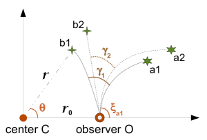
Let us assume now an expansion in a flat FRW space from a “center” observed by an off-center observer at a distance from . Since we are assuming FRW it is clear that any point in space could be considered a “center” of expansion: it is only when we will consider a LTB universe that the center acquires an absolute meaning. The relation between the observer line-of-sight angle and the coordinates of a source located at a radial distance and angle in the -frame is
| (1) |
where all angles are measured with respect to the axis and all distances in this section are to be understood as physical distances.
We consider first two sources at location on the same plane that includes the axis with an angular separation as seen from , both at distance from (throughout this letter we shall always assume for simplicity that both sources share the same coordinate). After some time , the sources move to positions and the distances and will have increased by and respectively. If for a moment we allow ourselves the liberty of assigning to the scale factor and the function a spatial dependence, a time-variation of is induced. The variation is the anticipated cosmic parallax effect and can be easily estimated if we suppose that the Hubble law is just generalized to . Generalizing to sources on different shells separated by a small (not to be mistaken with the time interval ) and , after straightforward geometry we arrive at
| (2) | ||||
where , (at this order we can neglect the difference between the observed angle and ). We can also convert the above intervals into the redshift interval by using the relations and , which combine to (we impose ), where .
In a FRW metric, does not depend on and the parallax vanishes. On the other hand, any deviation from FRW entails such spatial dependence and the emergence of cosmic parallax, except possibly for special observers (such as the center of LTB). A constraint on is therefore a constraint on cosmic anisotropy.
Rigorously, one actually needs to perform a full integration of light-ray geodesics in the new metric. Nevertheless, we shall assume for a moment that for an order of magnitude estimate we can simply replace with its space-dependent counterpart given by LTB models. In order for a LTB cosmology to have any substantial effect (e.g., explaining the SNIa Hubble diagram) it is reasonable to assume a difference between the local and the distant of order Alnes and Amarzguioui (2006). More precisely, putting then one has that the overall effect for on-shell sources is of order . That is, as anticipated, for years we expect a parallax of as for sources separated by . Similarly, for radial source pairs, neglecting the term (which is valid except close to the edge of the LTB void), one has as (assuming ).
Let us finally consider the main expected source of noise, the intrinsic peculiar velocities of the sources. The variation in angular separation for sources at angular diameter distance (measured by the observer) and peculiar velocity can be estimated as
| (3) |
This velocity field noise is therefore typically smaller than the experimental uncertainty (especially for large distances) and again will be averaged out for many sources. Notice that the observer’s own peculiar velocity produces a systematic offset sinusoidal signal of the same amplitude as that has to be subtracted from the observations: we discuss this further below.
Geodesic Equations. These very suggestive but simplistic calculations need confirmation from an exact treatment where the full relativistic propagation of light rays is taken into account. We will thus consider in what follows two particular LTB models capable of fitting the observed SNIa Hubble diagram and the CMB first peak position and compatible with the COBE results of the CMB dipole anisotropy, as long as the observer is within around 15 Mpc from the center Alnes and Amarzguioui (2006). Moreover, both models have void sizes which are small enough () not to be ruled out due to distortions of the CMB blackbody radiation spectrum Caldwell and Stebbins (2008).
The LTB metric can be written as (primes and dots refer to partial space and time derivatives, respectively):
| (4) |
where can be loosely thought as position dependent spatial curvature term. Two distinct Hubble parameters corresponding to the radial and perpendicular directions of expansion are defined as and (in a FRW metric and ). This class of models exhibits implicit analytic solutions of the Einstein equations in the case of a matter-dominated universe, to wit (in terms of a parameter )
| (5) | ||||
| (6) |
where , and , and are all functions of . In fact, stands for and we will choose to correspond to the time of last scattering, while is an arbitrary function and is assumed to be positive. Due to the axial symmetry and the fact that photons follow a path which preserves the 4-velocity identity , the four second-order geodesic equations for can be written as five first-order ones. We will choose as variables the center-based coordinates , , , and the redshift , where is the affine parameter of the geodesics. We shall refer also to the conserved angular momentum . For a particular source, the angle is the coordinate equivalent to for the observer, and in particular is the coordinate of a photon that arrives at the observer at the time of observation . Obviously this coincides with the measured position in the sky of such a source at . In terms of these variables, and defining such that , the autonomous system governing the geodesics is written as
| (7) | ||||
Following Alnes and Amarzguioui (2006), the angle along a geodesic is given by , from which we obtain and . Therefore, our system is completely defined by the initial conditions , , , and . The first two define the instant of measurement and the offset between observer and center, while stands for the direction of incidence of the photons. By integrating the geodesic equations for two sources located at after a time interval the CP will be .
The models of Ref. Alnes and Amarzguioui (2006) are characterized by a smooth transition between an inner void and an outer region with higher matter density and are described by the functions and (Eqs. (28) and (29) in Alnes and Amarzguioui (2006)), themselves carrying a total of 4 free parameters, one of which the value of the Hubble constant at the outer region, set at 51 km/(s Mpc). Following Alnes and Amarzguioui (2006) we dub them Model I and II; the main difference between them is that Model II features a sharper transition from the void. However transition width is not expected to be an important factor in CP since most quasars are outside the void and the most relevant quantity is the difference between the inner and outer values of . In both cases we set the off-center (physical) distance to 15 Mpc, which is the upper limit allowed by CMB dipole distortions Alnes and Amarzguioui (2006),and this corresponds to for a source at . It can be shown that in a step-like LTB void model, the in (2) is given by , whereas .
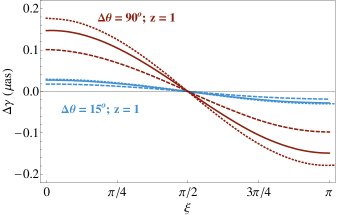
In Figure 2 we plot for three sources at , for models I and II as well as for the FRW-like estimate. One can see that the results do not depend sensitively on the details of the shell transition and that in both cases the FRW-like estimate gives a reasonable idea of the true LTB behavior. We conclude that (2) is a valid approximation. Numerically, we find that a convenient estimate of the parallax is given by as. For the LTB models above .
Integrating (7) yields also another interesting observable, , coupled to the CP: together they form a new set of real-time cosmic observables. Ref. Uzan et al. (2008a) calculated for an observer at the center of a LTB model. In the limit of small our numerical results reveal that for off-center observers show very small angular dependence.
Cosmic parallax with Gaia. A realistic possibility of observing the CP is offered by the forthcoming Gaia mission. Gaia will produce in five years a full-sky map of roughly quasars; by making of order 100 repeated measurements over the five years mission, Gaia will hopefully achieve a positional error between to as (for quasars with magnitude to ). To compare our observations to Gaia we need to evaluate the average with years and sources. The final Gaia error is obtained by best-fitting independent coordinates from angular separation measures; the average positional error on the entire sky will scale therefore as . Over one hemisphere we can therefore estimate that the error scales as . Since the average angular separation of random points on a sphere is , the average of can be estimated simply as . We find numerically as, with little dependence on . Therefore Gaia can see the parallax if as. For (i.e. the current CMB limit) and as we need sources: this shows that Gaia can constrain the cosmic anisotropy to CMB levels. An enhanced Gaia mission with years (or two missions 5 years apart), as and would give , i.e. Mpc if we assume the sources are at 2 Gpc. Two caveats of this preliminary estimate are however to be kept in mind. First, to map the angular change, Gaia’s observing strategy should be redesigned in order to maximize the time interval between quasar observations. Second, being planned to monitor the local matter distribution, Gaia’s errors estimates are based on using a fraction of the quasars as a reference frame. Observing the quasar CP would require a different statistical analysis. Both effects are likely to increase the expected final error.
Two local effects induce spurious parallaxes: one (of the order of 0.1as) is induced by our own peculiar velocity and the other (of the order of 4asKovalevsky (2003) by a changing aberration. Both produce a dipolar signal, just like a LTB: however, the peculiar velocity parallax decreases monotonically with the angular diameter distance, while the aberration change is independent of distance Kovalevsky (2003). In contrast, the LTB signal has a characteristic non-trivial dependence on redshift: for the models investigated here it is vanishingly small inside the void, large near the edge, decreasing at large distances. It is therefore possible in principle to subtract the cosmic signal from the local one, for instance estimating the local effects from sources inside the void, including Milky Way stars. A detailed calculation needs a careful simulation of experimental settings (including possibly effects like source photocenter jitter and relativistic light deflection by solar system bodies) which is outside the scope of this paper. Moreover, more general anisotropic models will not produce a simple dipole.
Conclusions. Planned space-based astrometric missions aim at accuracies of the order of few microarcseconds. In this paper we have shown that the cosmic parallax of distant sources in an LTB model might be observable employing the same missions. Similar considerations would apply to all other anisotropic cosmological models as e.g. the Bianchi models. A positive detection of large-scale CP would disprove therefore one of the basic tenets of modern cosmology, isotropy. We have shown that for a typical LTB model designed to explain the supernovae Ia Hubble diagram a enhanced Gaia experiment could constrain the anisotropy parameter to less than , corresponding to the Megaparsec scale, much better than current CMB dipole limits Alnes and Amarzguioui (2006). Moreover, this test may probe a different range of scales depending on the quasar redshift distribution and, contrary to the CMB limits, the CP method cannot be completely undermined by the observer’s peculiar motion and is limited only by source statistics instead of by the cosmic variance. We anticipate however that the major source of systematics would be the subtraction of the aberration change parallax. Real-time cosmology tests directly cosmic kinematics by observing changes in source positions and velocities. We have shown that the cosmic parallax, along with the velocity shift effect , can fully reconstruct the 3D cosmic flow of distant sources.
Acknowledgment. We thank A. Balbi, R. Scaramella and S. Bonometto for interesting discussions. MQ thanks Università di Milano-Bicocca for support.
References
- Célérier (2007) M.-N. Célérier, astro-ph/0702416 (2007).
- Marra et al. (2007) V. Marra, E. W. Kolb, S. Matarrese, and A. Riotto, Phys. Rev. D 76, 123004 (2007), eprint arXiv:0708.3622.
- Alexander et al. (2007) S. Alexander, T. Biswas, A. Notari, and D. Vaid, arXiv:0712.0370 (2007).
- Clarkson et al. (2008) C. Clarkson, B. Bassett, and T. H.-C. Lu, Physical Review Letters 101, 011301 (2008), eprint arXiv:0712.3457.
- Alnes and Amarzguioui (2006) H. Alnes and M. Amarzguioui, Phys. Rev. D 74, 103520 (2006), eprint arXiv:astro-ph/0607334.
- Garcia-Bellido and Haugbølle (2008) J. Garcia-Bellido and T. Haugbølle, Journal of Cosmology and Astro-Particle Physics 4, 3 (2008).
- Clifton et al. (2008) T. Clifton, P. G. Ferreira, and K. Land, arXiv:0807.1443 (2008).
- Humphreys et al. (1997) N. P. Humphreys, R. Maartens, and D. R. Matravers, Astrophys. J. 477, 47 (1997), eprint arXiv:astro-ph/9602033.
- Sandage (1962) A. Sandage, ApJ 136, 319 (1962).
- Loeb (1998) A. Loeb, ApJ 499, L111+ (1998), eprint astro-ph/9802122.
- Lake (2007) K. Lake, Phys. Rev. D 76, 063508 (2007).
- Balbi and Quercellini (2007) A. Balbi and C. Quercellini, MNRAS 382, 1623 (2007).
- Corasaniti et al. (2007) P.-S. Corasaniti, D. Huterer, and A. Melchiorri, Phys. Rev. D 75, 062001 (2007), eprint astro-ph/0701433.
- Uzan et al. (2008a) J.-P. Uzan, C. Clarkson, and G. F. R. Ellis, Physical Review Letters 100, 191303 (2008a), eprint arXiv:0801.0068.
- Uzan et al. (2008b) J.-P. Uzan, F. Bernardeau, and Y. Mellier, Phys. Rev. D 77, 021301 (2008b), eprint arXiv:0711.1950.
- Bailer-Jones (2005) C. A. L. Bailer-Jones, in IAU Colloq. 196, edited by D. W. Kurtz (2005), pp. 429–443.
- Goullioud et al. (2008) R. Goullioud, J. H. Catanzarite, F. G. Dekens, M. Shao, and J. C. Marr IV, arXiv:0807.1668 (2008).
- Yano et al. (2008) T. Yano, N. Gouda, Y. Kobayashi, Y. Yamada, T. Tsujimoto, M. Suganuma, Y. Niwa, and M. Yamauchi, in IAU Symposium (2008), vol. 248, pp. 296–297.
- Murata et al. (2007) Y. Murata, N. Mochizuki, H. Saito, H. Hirabayashi, M. Inoue, H. Kobayashi, and P. G. Edwards, in IAU Symposium (2007), vol. 242, pp. 517–521.
- Caldwell and Stebbins (2008) R. R. Caldwell and A. Stebbins, Physical Review Letters 100, 191302 (2008), eprint arXiv:0711.3459.
- Kovalevsky (2003) J. Kovalevsky, A&A 404, 743 (2003).