A detailed analysis of structure growth in f(R)𝑓𝑅f(R) theories of gravity

Kishore N. Ananda Department of Mathematics and Applied Mathematics, University of Cape Town, South Africa.    Sante Carloni Department of Mathematics and Applied Mathematics, University of Cape Town, South Africa.    Peter K S Dunsby Department of Mathematics and Applied Mathematics, University of Cape Town, South Africa.  South African Astronomical Observatory, Observatory Cape Town, South Africa.
Abstract

We investigate the connection between dark energy and fourth order gravity by analyzing the behavior of scalar perturbations around a Friedmann-Robertson-Walker background. The evolution equations for scalar perturbation are derived using the covariant and gauge invariant approach and applied to two widely studied f(R)𝑓𝑅f(R) gravity models. The structure of the general fourth order perturbation equations and the analysis of scalar perturbations lead to the discovery of a characteristic signature of fourth order gravity in the matter power spectrum, the details of which have not seen before in other works in this area. This could provide a crucial test for fourth order gravity on cosmological scales.

pacs:
04.50.+h, 04.25.Nx

I Introduction

In spite of all the efforts made so far, the problem of the nature of Dark Energy (DE) is still far from a completely satisfactory resolution. Among the many theoretical frameworks proposed, the idea of a geometrical origin of Dark Energy has recently received a great deal of attention. The main reason for this popularity can be found in the fact that these type of theories of gravity, which are suggested by the low energy limit of very fundamental schemes stringhe ; birrell , lead to cosmologies which admit naturally a Dark Energy era SalvSolo ; revnostra ; Odintsov ; Carroll ; star2007 (and possibly even an inflationary one kerner1 ; star80 ; Cognola1 ) without the introduction of any additional cosmological fields.

Much of the investigation performed up to now on the idea of Geometric Dark Energy has been focused on the so-called fourth order theories of gravity. In these theories the Hilbert-Einstein action is modified with terms that are at most of order four in the metric tensor. The features of fourth order gravity have been analyzed with different methods OurDynSys ; BarrowDyn ; Barrow Hervik ; OdintRec ; CognolaDyn and it has been shown that their cosmologies can give rise to a phase of accelerated expansion which is considered the footprint of Dark Energy.

Although these results are very encouraging there are still some important open problems to be addressed. One of them is the analysis of the evolution of the linear perturbations and their comparison with observations. Over the past year this problem has been studied by a number of authors, by (1) considering different ways of parameterizing the non-Einstein modifications of gravity or (2) by simplifying the underlying fourth-order perturbation equations using a quasi-static approximation or a combination of (1) and (2) Li:2008ai ; HuSawicki ; Bertschinger:2008zb ; otherperts .

In a number of recent papers SantePert ; K1 we derived the evolution equations for scalar and tensor perturbations of a subclass of fourth order theories of gravity characterized by an action which is a general analytic function of the Ricci scalar. In our work we study the dynamics of linear scalar perturbations using the covariant and gauge invariant approach developed for General Relativity (GR) in EllisCovariant ; EB ; EBH ; BDE ; DBE ; BED ; DBBE . This approach has the advantage of using perturbation variables with a clear geometrical and physical interpretation. Furthermore, we use a specific recasting of the field equations that will make the development of the cosmological perturbation theory even more transparent, allowing one to integrate the perturbation equations exactly for a given f(R)𝑓𝑅f(R) model without making any additional approximations.

The preliminary results obtained in SantePert showed some interesting features. First of all the evolution of scalar perturbations is determined by a fourth order differential equation rather than a second order one. This implies that the evolution of the density fluctuations contains, in general, four modes rather that two and can give rise to a more complex evolution than the one of General Relativity (GR). Secondly, the perturbations are found to depend on the scale for any equation of state for standard matter (while in GR the evolution of the dust perturbations are not scale dependent). This means that, for example, in this framework the evolution of super-horizon and sub-horizon perturbations is different. Third, and more surprisingly, we found that growth of large density fluctuations can occur also in backgrounds in which the expansion rate is increasing in time. This is in striking contrast with what one finds in GR and what one would naively expect, but at the same time suggests new ways to tackle the DE problem.

The features mentioned above imply that the evolution of perturbations in this framework can be completely different from the one we are familiar with. Yet this does not necessarily mean that they are incompatible with observations. Rather, they are a sign of the fact that in dealing with these models one has to resist the temptation of using assumptions which work well in GR. In this paper, following in this spirit, we will analyze further what was found in SantePert with the aim of achieving a clearer understanding of the physics of the matter dominated era in fourth order gravity. In order to do this, we will rewrite the perturbation equations in a more physically meaningful way and will develop a series of tools which will make the analysis of the evolution of density perturbations easier to understand and to compare with GR.

The paper is organized as follows. In section II we will give some basic equations and we will present briefly the covariant gauge invariant formalism we use to develop the perturbation theory. In section III, we give the background and the perturbation equations. In section IV we rewrite these equation in an interesting form allowing us to discuss their general structure. In section V we propose some useful tools to understand the behavior of the perturbations and compare it with what one obtains in General Relativity. In section VI we apply these tools to some simple specific examples. Section VII is dedicated to the conclusions.

Unless otherwise specified, natural units (=c=kB=8πG=1Planck-constant-over-2-pi𝑐subscript𝑘𝐵8𝜋𝐺1\hbar=c=k_{B}=8\pi G=1) will be used throughout this paper, Latin indices run from 0 to 3. The symbol \nabla represents the usual covariant derivative and \partial corresponds to partial differentiation. We use the ,+,+,+-,+,+,+ signature and the Riemann tensor is defined by

Ra=bcdWabd,cWa+bc,dWeWabdceWfWabc,dfR^{a}{}_{bcd}=W^{a}{}_{bd,c}-W^{a}{}_{bc,d}+W^{e}{}_{bd}W^{a}{}_{ce}-W^{f}{}_{bc}W^{a}{}_{df}\;, (1)

where the WabdW^{a}{}_{bd} are the Christoffel symbols (i.e. symmetric in the lower indices), defined by

Wbda=12gae(gbe,d+ged,bgbd,e).subscriptsuperscript𝑊𝑎𝑏𝑑12superscript𝑔𝑎𝑒subscript𝑔𝑏𝑒𝑑subscript𝑔𝑒𝑑𝑏subscript𝑔𝑏𝑑𝑒W^{a}_{bd}=\frac{1}{2}g^{ae}\left(g_{be,d}+g_{ed,b}-g_{bd,e}\right)\;. (2)

The Ricci tensor is obtained by contracting the first and the third indices

Rab=gcdRacbd.subscript𝑅𝑎𝑏superscript𝑔𝑐𝑑subscript𝑅𝑎𝑐𝑏𝑑R_{ab}=g^{cd}R_{acbd}\;. (3)

Finally the Hilbert–Einstein action in the presence of matter is given by

𝒜=𝑑x4g[12R+Lm].𝒜differential-dsuperscript𝑥4𝑔delimited-[]12𝑅subscript𝐿𝑚{\cal A}=\int dx^{4}\sqrt{-g}\left[\frac{1}{2}R+L_{m}\right]\;. (4)

II General equations for fourth order gravity.

In four dimensional homogeneous and isotropic spacetimes i.e. Friedmann Lemaître Robertson Walker (FLRW) universes, the most general action for fourth order gravity can be written as an analytic function of the Ricci scalar only:

𝒜=d4xg[f(R)+m],𝒜superscript𝑑4𝑥𝑔delimited-[]𝑓𝑅subscript𝑚\mathcal{A}=\int d^{4}x\sqrt{-g}\left[f(R)+{\cal L}_{m}\right]\;, (5)

where msubscript𝑚\mathcal{L}_{m} represents the matter contribution. Varying the action with respect to the metric gives the generalization of the Einstein equations:

fGab=f(Rab12gabR)=Tabm+12gab(fRf)+bafgabccf,superscript𝑓subscript𝐺𝑎𝑏superscript𝑓subscript𝑅𝑎𝑏12subscript𝑔𝑎𝑏𝑅superscriptsubscript𝑇𝑎𝑏𝑚12subscript𝑔𝑎𝑏𝑓𝑅superscript𝑓subscript𝑏subscript𝑎superscript𝑓subscript𝑔𝑎𝑏subscript𝑐superscript𝑐superscript𝑓f^{\prime}G_{ab}=f^{\prime}\left(R_{ab}-\frac{1}{2}\,g_{ab}R\right)=T_{ab}^{m}+\frac{1}{2}g_{ab}\left(f-Rf^{\prime}\right)+\nabla_{b}\nabla_{a}f^{\prime}-g_{ab}\nabla_{c}\nabla^{c}f^{\prime}\;, (6)

where f=f(R)𝑓𝑓𝑅f=f(R), f=df(R)drsuperscript𝑓𝑑𝑓𝑅𝑑𝑟f^{\prime}=\displaystyle{\frac{df(R)}{dr}}, and TabM=2gδ(gm)δgabsubscriptsuperscript𝑇𝑀𝑎𝑏2𝑔𝛿𝑔subscript𝑚𝛿subscript𝑔𝑎𝑏\displaystyle{T^{M}_{ab}=\frac{2}{\sqrt{-g}}\frac{\delta(\sqrt{-g}\mathcal{L}_{m})}{\delta g_{ab}}} represents the stress energy tensor of standard matter. These equations reduce to the standard Einstein field equations when f(R)=R𝑓𝑅𝑅f(R)=R. It is crucial for our purposes to be able to write (6) in the form

Gab=T~abm+TabR=Tabtot,subscript𝐺𝑎𝑏superscriptsubscript~𝑇𝑎𝑏𝑚subscriptsuperscript𝑇𝑅𝑎𝑏subscriptsuperscript𝑇𝑡𝑜𝑡𝑎𝑏G_{ab}=\tilde{T}_{ab}^{m}+T^{R}_{ab}=T^{tot}_{ab}\,, (7)

where T~abm=Tabmfsuperscriptsubscript~𝑇𝑎𝑏𝑚superscriptsubscript𝑇𝑎𝑏𝑚superscript𝑓\displaystyle{\tilde{T}_{ab}^{m}=\frac{T_{ab}^{m}}{f^{\prime}}} and

TabR=1f[12gab(fRf)+bafgabccf],superscriptsubscript𝑇𝑎𝑏𝑅1superscript𝑓delimited-[]12subscript𝑔𝑎𝑏𝑓𝑅superscript𝑓subscript𝑏subscript𝑎𝑓subscript𝑔𝑎𝑏subscript𝑐superscript𝑐𝑓\displaystyle T_{ab}^{R}=\frac{1}{f^{\prime}}\left[\frac{1}{2}g_{ab}\left(f-Rf^{\prime}\right)+\nabla_{b}\nabla_{a}f-g_{ab}\nabla_{c}\nabla^{c}f\right], (8)

represent two effective “fluids”: the curvature “fluid”111Some authors have recently adopted the name Effective Dark Matter for the curvature fluid Li:2008ai . (associated with TabRsubscriptsuperscript𝑇𝑅𝑎𝑏T^{R}_{ab}) and the effective matter “fluid” (associated with T~abmsuperscriptsubscript~𝑇𝑎𝑏𝑚\tilde{T}_{ab}^{m}) SalvSolo ; revnostra ; SantePert . This step is important because it allows us to treat fourth order gravity as standard Einstein gravity plus two “effective” fluids. The details of the conservation properties of these effective fluids have been given in SantePert . In particular, it has been shown that, no matter how the effective fluids behave, standard matter still follows the usual conservation equations Tabm;b=0superscriptsubscript𝑇𝑎𝑏𝑚𝑏0T_{ab}^{m\ ;b}=0.

The form (7) of the field equations allows us to use directly the covariant gauge invariant approach EllisCovariant ; EB ; EBH ; DBE ; BED ; BDE ; DBBE in the same way presented in SantePert . As usual the first step is to choose suitable frame, i.e., a 4-velocity uasubscript𝑢𝑎u_{a} of an observer in spacetime. Following SantePert , we will choose this frame to be the one comoving with standard matter, which is also called matter energy frame and will be indicated in the following by uamsubscriptsuperscript𝑢𝑚𝑎u^{m}_{a}. We will also assume that in uamsubscriptsuperscript𝑢𝑚𝑎u^{m}_{a} standard matter is a barotropic perfect fluid with equation of state p=wρ𝑝𝑤𝜌p=w\rho. Since the real observers are attached to galaxies and the galaxies follow the standard matter geodesics, this frame choice appears to be best motivated from a physical point of view.

Once the frame has been chosen the derivation of the kinematical quantities can be obtained in a standard way EllisCovariant . In particular the derivative along the matter fluid flow lines is defined by X˙=uaaX˙𝑋subscript𝑢𝑎superscript𝑎𝑋\dot{X}=u_{a}\nabla^{a}X and the projected covariant derivative operator orthogonal to uasuperscript𝑢𝑎u^{a} is given by ~a=hbba\tilde{\nabla}_{a}=h^{b}{}_{a}\nabla_{b}. With these definitions we can define the key kinematic quantities of the cosmological model: the expansion ΘΘ\Theta, the shear σabsubscript𝜎𝑎𝑏\sigma_{ab}, the vorticity ωabsubscript𝜔𝑎𝑏\omega_{ab} and the acceleration aa=u˙asubscript𝑎𝑎subscript˙𝑢𝑎a_{a}=\dot{u}_{a}. The general propagation equations for these kinematic variables in any spacetime correspond to the so called 1+3 covariant equations EllisCovariant which are given in Appendix A.

The definition of a frame uasubscript𝑢𝑎u_{a} also allows us to obtain an irreducible decomposition of the stress energy momentum tensor. In a general frame and for a general tensor Tabsubscript𝑇𝑎𝑏T_{{a}{{b}}} one obtains:

Tab=μuaub+phab+2q(aub)+πab,T_{{a}{{b}}}=\mu u_{a}u_{{b}}+ph_{{a}{{b}}}+2q_{(a}u_{{{b}})}+\pi_{{{a}}{{b}}}\,, (9)

where μ𝜇\mu and p𝑝p are the energy density and isotropic pressure, qasubscript𝑞𝑎q_{{{a}}} is the energy flux (qa=qasubscript𝑞𝑎subscript𝑞delimited-⟨⟩𝑎q_{{{a}}}=q_{\langle{{a}}\rangle}) and πabsubscript𝜋𝑎𝑏\pi_{{{a}}{{b}}} is the anisotropic pressure (πab=πabsubscript𝜋𝑎𝑏subscript𝜋delimited-⟨⟩𝑎𝑏\pi_{{{a}}{{b}}}=\pi_{\langle{{a}}{{b}}\rangle}).

In this way, relative to uamsuperscriptsubscript𝑢𝑎𝑚u_{a}^{m}, Tabtotsubscriptsuperscript𝑇𝑡𝑜𝑡𝑎𝑏T^{tot}_{ab} can be decomposed as

μtotsuperscript𝜇tot\displaystyle\mu^{\rm tot}\, =\displaystyle= Tabtotuaub=μ~m+μR,ptot=13Tabtothab=p~m+pR,formulae-sequencesubscriptsuperscript𝑇tot𝑎𝑏superscript𝑢𝑎superscript𝑢𝑏superscript~𝜇𝑚superscript𝜇𝑅superscript𝑝tot13subscriptsuperscript𝑇tot𝑎𝑏superscript𝑎𝑏superscript~𝑝𝑚superscript𝑝𝑅\displaystyle T^{\rm tot}_{ab}u^{a}u^{b}\,=\,\tilde{\mu}^{\,m}+\mu^{\,R}\,,\qquad p^{\rm tot}\,=\frac{1}{3}T^{\rm tot}_{ab}h^{ab}\,=\,\tilde{p}^{\,m}+p^{\,R}\;, (10)
qatotsubscriptsuperscript𝑞tot𝑎\displaystyle q^{\rm tot}_{a}\, =\displaystyle= Tbctothabuc=q~am+qaR,πabtot=Tcdtoth<achb>d=π~abm+πabR,formulae-sequencesubscriptsuperscript𝑇tot𝑏𝑐superscriptsubscript𝑎𝑏superscript𝑢𝑐subscriptsuperscript~𝑞𝑚𝑎subscriptsuperscript𝑞𝑅𝑎subscriptsuperscript𝜋tot𝑎𝑏subscriptsuperscript𝑇tot𝑐𝑑superscriptsubscriptabsent𝑎𝑐superscriptsubscript𝑏absent𝑑subscriptsuperscript~𝜋𝑚𝑎𝑏subscriptsuperscript𝜋𝑅𝑎𝑏\displaystyle-T^{\rm tot}_{bc}h_{a}^{b}u^{c}\,=\,\tilde{q}^{\,m}_{a}+q^{\,R}_{a}\,,\qquad\pi^{\rm tot}_{ab}\,=\,T^{\rm tot}_{cd}h_{<a}^{c}h_{b>}^{d}\,=\,\tilde{\pi}^{\,m}_{ab}+\pi^{\,R}_{ab}\,, (11)

with

μ~msuperscript~𝜇𝑚\displaystyle\tilde{\mu}^{\,m}\, =\displaystyle= μmf,p~m=pmf,q~am=qamf,π~abm=πabmf.formulae-sequencesuperscript𝜇𝑚superscript𝑓superscript~𝑝𝑚superscript𝑝𝑚superscript𝑓formulae-sequencesubscriptsuperscript~𝑞𝑚𝑎subscriptsuperscript𝑞𝑚𝑎superscript𝑓subscriptsuperscript~𝜋𝑚𝑎𝑏subscriptsuperscript𝜋𝑚𝑎𝑏superscript𝑓\displaystyle\,\frac{\mu^{\,m}}{f^{\prime}}\,,\qquad\tilde{p}^{\,m}\,=\,\frac{p^{\,m}}{f^{\prime}}\,,\qquad\tilde{q}^{\,m}_{a}\,=\,\frac{q^{\,m}_{a}}{f^{\prime}}\,,\qquad\tilde{\pi}^{\,m}_{ab}=\,\frac{\pi^{\,m}_{ab}}{f^{\prime}}\,. (12)

Since we assume that standard matter is a perfect fluid in uamsuperscriptsubscript𝑢𝑎𝑚u_{a}^{m}, qamsubscriptsuperscript𝑞𝑚𝑎q^{\,m}_{a} and πabmsubscriptsuperscript𝜋𝑚𝑎𝑏\pi^{\,m}_{ab} are zero, so that the last two quantities above also vanish.

The effective thermodynamical quantities for the curvature “fluid” are

μR=1f[12(Rff)Θf′′R˙+f′′~2R+f′′ab~bR],superscript𝜇𝑅1superscript𝑓delimited-[]12𝑅superscript𝑓𝑓Θsuperscript𝑓′′˙𝑅superscript𝑓′′superscript~2𝑅superscript𝑓′′subscript𝑎𝑏superscript~𝑏𝑅\displaystyle\mu^{R}\,=\,\frac{1}{f^{\prime}}\left[\frac{1}{2}(Rf^{\prime}-f)-\Theta f^{\prime\prime}\dot{R}+f^{\prime\prime}\tilde{\nabla}^{2}{R}+f^{\prime\prime}\,a_{b}\tilde{\nabla}^{b}{R}\right]\;, (13)
pR=1f[12(fRf)+f′′R¨+f′′′R˙2+23Θf′′R˙23f′′~2R+\displaystyle p^{R}\,=\,\frac{1}{f^{\prime}}\left[\frac{1}{2}(f-Rf^{\prime})+f^{\prime\prime}\ddot{R}+f^{\prime\prime\prime}\dot{R}^{2}+\frac{2}{3}\Theta f^{\prime\prime}\dot{R}-\frac{2}{3}f^{\prime\prime}\tilde{\nabla}^{2}{R}+\right.
23f′′′~aR~aR13f′′ab~bR],\displaystyle\qquad\left.-\frac{2}{3}f^{\prime\prime\prime}\tilde{\nabla}^{a}{R}\tilde{\nabla}_{a}{R}-\frac{1}{3}f^{\prime\prime}\,a_{b}\tilde{\nabla}^{b}{R}\right]\;, (14)
qaR=1f[f′′′R˙~aR+f′′~aR˙13Θf′′~aR],subscriptsuperscript𝑞𝑅𝑎1superscript𝑓delimited-[]superscript𝑓′′′˙𝑅subscript~𝑎𝑅superscript𝑓′′subscript~𝑎˙𝑅13Θsuperscript𝑓′′subscript~𝑎𝑅\displaystyle q^{R}_{a}\,=\,-\frac{1}{f^{\prime}}\left[f^{\prime\prime\prime}\dot{R}\tilde{\nabla}_{a}R+f^{\prime\prime}\tilde{\nabla}_{a}\dot{R}-\frac{1}{3}\Theta f^{\prime\prime}\tilde{\nabla}_{a}R\right]\;, (15)
πabR=1f[f′′~a~bR+f′′′~aR~bRσabR˙].\displaystyle\pi^{R}_{ab}\,=\,\frac{1}{f^{\prime}}\left[f^{\prime\prime}\tilde{\nabla}_{\langle a}\tilde{\nabla}_{b\rangle}R+f^{\prime\prime\prime}\tilde{\nabla}_{\langle a}{R}\tilde{\nabla}_{b\rangle}{R}-\sigma_{ab}\dot{R}\right]\,. (16)

The twice contracted Bianchi Identities lead to evolution equations for μmsuperscript𝜇𝑚\mu^{\,m}, μRsuperscript𝜇𝑅\mu^{R}, qaRsubscriptsuperscript𝑞𝑅𝑎q^{R}_{a} and are given in Appendix A.

III Linearized Scalar Perturbations Equations

Using the quantities defined above, and the equations given in Appendix A, we are able to write both the evolution equations for the background and ones for scalar perturbations. As in SantePert we will consider a background that is homogeneous and isotropic, i.e., a FLRW model. In this background the cosmological equations for a generic f(R)𝑓𝑅f(R) read:

Θ2= 3μ~m+3μR3R~2,superscriptΘ23superscript~𝜇𝑚3superscript𝜇𝑅3~𝑅2\displaystyle\Theta^{2}\,=\,3\tilde{\mu}^{m}+3\mu^{R}-\frac{3\tilde{R}}{2}\;, (17)
Θ˙+13Θ2+12(μ~m+3p~m)+12(μR+3pR)=0,˙Θ13superscriptΘ212superscript~𝜇𝑚3superscript~𝑝𝑚12superscript𝜇𝑅3superscript𝑝𝑅0\displaystyle\dot{\Theta}+{\textstyle\frac{1}{3}}\Theta^{2}+{\textstyle\frac{1}{2}}(\tilde{\mu}^{m}+3\tilde{p}^{m})+{\textstyle\frac{1}{2}}({\mu}^{R}+3{p}^{R})=0\;, (18)
μ˙m+Θ(μm+pm)=0,superscript˙𝜇𝑚Θsuperscript𝜇𝑚superscript𝑝𝑚0\displaystyle\dot{\mu}^{m}\,+\,\Theta\,(\mu^{m}+{p^{m}})=0\;, (19)

where R~=6K/S2~𝑅6𝐾superscript𝑆2\tilde{R}=6K/S^{2} is the 3-Ricci scalar, K=0,±1𝐾0plus-or-minus1K=0,\pm 1 and S𝑆S is the scale factor. The structure of these equations shows clearly that the effect of the introduction of higher order gravity on the background has a twofold nature. On one side, higher order gravity behaves like a an additional fluid in the model. On the other, it influences the way in which standard matter interacts gravitationally.

Following SantePert , we characterize scalar perturbations using the variables

Δam=S2μm~2μm,Z=S2~2Θ,C=S3~2R~,=S2~2R,=S2~aR˙,formulae-sequencesubscriptsuperscriptΔ𝑚𝑎superscript𝑆2superscript𝜇𝑚superscript~2superscript𝜇𝑚formulae-sequence𝑍superscript𝑆2superscript~2Θformulae-sequence𝐶superscript𝑆3superscript~2~𝑅formulae-sequencesuperscript𝑆2superscript~2𝑅superscript𝑆2subscript~𝑎˙𝑅\Delta^{m}_{{a}}=\frac{S^{2}}{\mu^{m}}\tilde{\nabla}^{2}\mu^{m}\,,\qquad Z=S^{2}\tilde{\nabla}^{2}\Theta\,,\qquad C=S^{3}\tilde{\nabla}^{2}\tilde{R}\,,\qquad{\cal R}=S^{2}\tilde{\nabla}^{2}R\,,\qquad\Re=S^{2}\tilde{\nabla}_{{a}}\dot{R}\;, (20)

the first three variables, which are borrowed from GR, represent the scalar fluctuations in the matter energy density, in the expansion rate (which is associated with μ˙˙𝜇\dot{\mu}) and in the spatial curvature. The last two represent the fluctuation of the Ricci scalar and its momentum.

It is a relatively easy task to derive the propagation equations for these variables in a FLRW background. Their form is Appendix B. If we focus on the evolution of scalar part of these variables, which is associated with the spherically symmetric collapse terms, these equations become

Δ˙m=wΘΔm(1+w)Z,subscript˙Δ𝑚𝑤ΘsubscriptΔ𝑚1𝑤𝑍\displaystyle\dot{\Delta}_{m}=w\Theta\Delta_{m}-(1+w)Z\,, (21)
Z˙=(R˙f′′f2Θ3)Z+[(w1)(3w+2)2(w+1)μf+2wΘ2+3w(μR+3pR)6(w+1)]Δm+Θf′′f+˙𝑍˙𝑅superscript𝑓′′superscript𝑓2Θ3𝑍delimited-[]𝑤13𝑤22𝑤1𝜇superscript𝑓2𝑤superscriptΘ23𝑤superscript𝜇𝑅3superscript𝑝𝑅6𝑤1subscriptΔ𝑚limit-fromΘsuperscript𝑓′′superscript𝑓\displaystyle\dot{Z}=\left(\frac{\dot{R}f^{\prime\prime}}{f^{\prime}}-\frac{2\Theta}{3}\right)Z+\left[\frac{(w-1)(3w+2)}{2(w+1)}\frac{\mu}{f^{\prime}}+\frac{2w\Theta^{2}+3w(\mu^{R}+3p^{R})}{6(w+1)}\right]\Delta_{m}+\frac{\Theta f^{\prime\prime}}{f^{\prime}}\Re+
+[1212fff′′ff′′fμf+R˙Θ(f′′f)2+R˙Θf(3)f]ww+1~2Δmf′′f~2,delimited-[]1212𝑓superscript𝑓superscript𝑓′′superscript𝑓superscript𝑓′′superscript𝑓𝜇superscript𝑓˙𝑅Θsuperscriptsuperscript𝑓′′superscript𝑓2˙𝑅Θsuperscript𝑓3superscript𝑓𝑤𝑤1superscript~2subscriptΔ𝑚superscript𝑓′′superscript𝑓superscript~2\displaystyle+\left[\frac{1}{2}-\frac{1}{2}\frac{f}{f^{\prime}}\frac{f^{\prime\prime}}{f^{\prime}}-\frac{f^{\prime\prime}}{f^{\prime}}\frac{\mu}{f^{\prime}}+\dot{R}\Theta\left(\frac{f^{\prime\prime}}{f^{\prime}}\right)^{2}+\dot{R}\Theta\frac{f^{(3)}}{f^{\prime}}\right]\mathcal{R}-\frac{w}{w+1}\tilde{\nabla}^{2}{\Delta}_{m}-\frac{f^{\prime\prime}}{f^{\prime}}\tilde{\nabla}^{2}\mathcal{R}\,, (22)
˙=ww+1R˙Δm,˙𝑤𝑤1˙𝑅subscriptΔ𝑚\displaystyle\dot{{\cal R}}=\Re-\frac{w}{w+1}\dot{R}\;{\Delta}_{m}\,, (23)
˙=(Θ+2R˙f(3)f′′)R˙Z[(3w1)3μf′′+w3(w+1)R¨]Δm+˙Θ2˙𝑅superscript𝑓3superscript𝑓′′˙𝑅𝑍limit-fromdelimited-[]3𝑤13𝜇superscript𝑓′′𝑤3𝑤1¨𝑅subscriptΔ𝑚\displaystyle\dot{\Re}=-\left(\Theta+2\dot{R}\frac{f^{(3)}}{f^{\prime\prime}}\right)\Re-\dot{R}Z-\left[\frac{(3w-1)}{3}\frac{\mu}{f^{\prime\prime}}+\frac{w}{3(w+1)}\ddot{R}\right]{\Delta}_{m}+
[13ff′′+f(4)fR˙2+ΘR˙f(3)f′′+R¨f(3)f′′R3]+~2,delimited-[]13superscript𝑓superscript𝑓′′superscript𝑓4superscript𝑓superscript˙𝑅2Θ˙𝑅superscript𝑓3superscript𝑓′′¨𝑅superscript𝑓3superscript𝑓′′𝑅3superscript~2\displaystyle-\left[\frac{1}{3}\frac{f^{\prime}}{f^{\prime\prime}}+\frac{f^{(4)}}{f^{\prime}}\dot{R}^{2}+\Theta\dot{R}\frac{f^{(3)}}{f^{\prime\prime}}+\ddot{R}\frac{f^{(3)}}{f^{\prime\prime}}-\frac{R}{3}\right]\mathcal{R}+\tilde{\nabla}^{2}\mathcal{R}\,, (24)
C˙=k2[18f′′S2Θf18ΔmS2Θ]+K[3S2ΘC+Δm(2(w1)Θw+1+6μRΘ)6f′′Θf′′~2+6f′′f+\displaystyle\dot{C}=k^{2}\left[\frac{18f^{\prime\prime}\mathcal{R}}{S^{2}\Theta f^{\prime}}-\frac{18\Delta_{m}}{S^{2}\Theta}\right]+K\left[\frac{3}{S^{2}\Theta}C+\Delta_{m}\left(\frac{2(w-1)\Theta}{w+1}+\frac{6\mu^{R}}{\Theta}\right)-\frac{6f^{\prime\prime}}{\Theta f^{\prime\prime}}\tilde{\nabla}^{2}\mathcal{R}+\frac{6f^{\prime\prime}}{f^{\prime}}\Re+\right.
+6R˙Θff(3)f′′(3f2(Θ23μR)f+6R˙Θf′′)Θ(f)2]+~2[4wS2Θ3(w+1)Δm+2S2f′′f2S2(Θf′′3R˙f(3))3f],\displaystyle\left.+\frac{6\dot{R}\Theta f^{\prime}f^{(3)}-f^{\prime\prime}\left(3f-2\left(\Theta^{2}-3\mu^{R}\right)f^{\prime}+6\dot{R}\Theta f^{\prime\prime}\right)}{\Theta(f^{\prime})^{2}}\mathcal{R}\right]+\tilde{\nabla}^{2}\left[\frac{4wS^{2}\Theta}{3(w+1)}\Delta_{m}+\frac{2S^{2}f^{\prime\prime}}{f^{\prime}}\Re-\frac{2S^{2}\left(\Theta f^{\prime\prime}-3\dot{R}f^{(3)}\right)}{3f^{\prime}}\mathcal{R}\right]\,,

together with the constraint

CS2+(43Θ+2R˙f′′f)Z2μfΔmm+[2R˙Θf(3)ff′′(f)2(f2μ+2R˙Θf′′)]+2Θf′′f2f′′f~2=0.𝐶superscript𝑆243Θ2˙𝑅superscript𝑓′′superscript𝑓𝑍2𝜇superscript𝑓subscriptsubscriptΔ𝑚𝑚delimited-[]2˙𝑅Θsuperscript𝑓3superscript𝑓superscript𝑓′′superscriptsuperscript𝑓2𝑓2𝜇2˙𝑅Θsuperscript𝑓′′2Θsuperscript𝑓′′superscript𝑓2superscript𝑓′′superscript𝑓superscript~20\frac{C}{S^{2}}+\left(\frac{4}{3}\Theta+\frac{2\dot{R}f^{\prime\prime}}{f^{\prime}}\right)Z-2\frac{\mu}{f^{\prime}}{\Delta_{m}}_{m}+\left[2\dot{R}\Theta\frac{f^{(3)}}{f^{\prime}}-\frac{f^{\prime\prime}}{(f^{\prime})^{2}}\left(f-2\mu+2\dot{R}\Theta f^{\prime\prime}\right)\right]\mathcal{R}+\frac{2\Theta f^{\prime\prime}}{f^{\prime}}\Re-\frac{2f^{\prime\prime}}{f^{\prime}}\tilde{\nabla}^{2}\mathcal{R}=0\,. (25)

Note that this system is made up of four first order differential equation, which means that the evolution of every single perturbation variable is determined by a fourth order differential equation. This has a profound influence in the dynamics of the perturbations and makes them potentially very different from what one obtains in standard GR.

Traditionally the analysis of the perturbation equations is simplified by using a harmonic decomposition. In the 1+3 formalism this can be done by developing the scalar quantities defined above using the eigenfunctions of the Laplace-Beltrami operator BDE :

~2Q=k2S2Q,superscript~2𝑄superscript𝑘2superscript𝑆2𝑄\displaystyle\tilde{\nabla}^{2}Q=-\frac{k^{2}}{S^{2}}Q\;, (26)

where k=2πS/λ𝑘2𝜋𝑆𝜆k=2\pi S/\lambda is the wavenumber and Q˙=0˙𝑄0\dot{Q}=0. Developing (20) in terms of Q𝑄Q, (21-25) reduce to

Δ˙m(k)superscriptsubscript˙Δ𝑚𝑘\displaystyle\dot{\Delta}_{m}^{(k)} =\displaystyle= wΘΔm(k)(1+w)Z(k),𝑤ΘsuperscriptsubscriptΔ𝑚𝑘1𝑤superscript𝑍𝑘\displaystyle w\Theta\Delta_{m}^{(k)}-(1+w)Z^{(k)}\,, (27)
Z˙(k)superscript˙𝑍𝑘\displaystyle\dot{Z}^{(k)} =\displaystyle= (R˙f′′f2Θ3)Z(k)+[(w1)(3w+2)2(w+1)μf+2wΘ2+3w(μR+3pR)6(w+1)]Δm(k)+Θf′′f(k)+˙𝑅superscript𝑓′′superscript𝑓2Θ3superscript𝑍𝑘delimited-[]𝑤13𝑤22𝑤1𝜇superscript𝑓2𝑤superscriptΘ23𝑤superscript𝜇𝑅3superscript𝑝𝑅6𝑤1superscriptsubscriptΔ𝑚𝑘limit-fromΘsuperscript𝑓′′superscript𝑓superscript𝑘\displaystyle\left(\frac{\dot{R}f^{\prime\prime}}{f^{\prime}}-\frac{2\Theta}{3}\right)Z^{(k)}+\left[\frac{(w-1)(3w+2)}{2(w+1)}\frac{\mu}{f^{\prime}}+\frac{2w\Theta^{2}+3w(\mu^{R}+3p^{R})}{6(w+1)}\right]\Delta_{m}^{(k)}+\frac{\Theta f^{\prime\prime}}{f^{\prime}}\Re^{(k)}+ (28)
+[12f′′fk2S212fff′′ff′′fμf+R˙Θ(f′′f)2+R˙Θf(3)f](k),delimited-[]12superscript𝑓′′superscript𝑓superscript𝑘2superscript𝑆212𝑓superscript𝑓superscript𝑓′′superscript𝑓superscript𝑓′′superscript𝑓𝜇superscript𝑓˙𝑅Θsuperscriptsuperscript𝑓′′superscript𝑓2˙𝑅Θsuperscript𝑓3superscript𝑓superscript𝑘\displaystyle+\left[\frac{1}{2}-\frac{f^{\prime\prime}}{f^{\prime}}\frac{k^{2}}{S^{2}}-\frac{1}{2}\frac{f}{f^{\prime}}\frac{f^{\prime\prime}}{f^{\prime}}-\frac{f^{\prime\prime}}{f^{\prime}}\frac{\mu}{f^{\prime}}+\dot{R}\Theta\left(\frac{f^{\prime\prime}}{f^{\prime}}\right)^{2}+\dot{R}\Theta\frac{f^{(3)}}{f^{\prime}}\right]\mathcal{R}^{(k)}\,,
˙(k)superscript˙𝑘\displaystyle\dot{{\cal R}}^{(k)} =\displaystyle= (k)ww+1R˙Δm(k),superscript𝑘𝑤𝑤1˙𝑅superscriptsubscriptΔ𝑚𝑘\displaystyle\Re^{(k)}-\frac{w}{w+1}\dot{R}\;{\Delta}_{m}^{(k)}\,, (29)
˙(k)superscript˙𝑘\displaystyle\dot{\Re}^{(k)} =\displaystyle= (Θ+2R˙f(3)f′′)(k)R˙Z(k)[(3w1)3μf′′+w3(w+1)R¨]Δm(k)+Θ2˙𝑅superscript𝑓3superscript𝑓′′superscript𝑘˙𝑅superscript𝑍𝑘limit-fromdelimited-[]3𝑤13𝜇superscript𝑓′′𝑤3𝑤1¨𝑅superscriptsubscriptΔ𝑚𝑘\displaystyle-\left(\Theta+2\dot{R}\frac{f^{(3)}}{f^{\prime\prime}}\right)\Re^{(k)}-\dot{R}Z^{(k)}-\left[\frac{(3w-1)}{3}\frac{\mu}{f^{\prime\prime}}+\frac{w}{3(w+1)}\ddot{R}\right]{\Delta}_{m}^{(k)}+ (30)
+[k2S2(13ff′′+f(4)fR˙2+ΘR˙f(3)f′′+R¨f(3)f′′R3)](k),delimited-[]superscript𝑘2superscript𝑆213superscript𝑓superscript𝑓′′superscript𝑓4superscript𝑓superscript˙𝑅2Θ˙𝑅superscript𝑓3superscript𝑓′′¨𝑅superscript𝑓3superscript𝑓′′𝑅3superscript𝑘\displaystyle+\left[\frac{k^{2}}{S^{2}}-\left(\frac{1}{3}\frac{f^{\prime}}{f^{\prime\prime}}+\frac{f^{(4)}}{f^{\prime}}\dot{R}^{2}+\Theta\dot{R}\frac{f^{(3)}}{f^{\prime\prime}}+\ddot{R}\frac{f^{(3)}}{f^{\prime\prime}}-\frac{R}{3}\right)\right]\mathcal{R}^{(k)}\,,
C˙(k)superscript˙𝐶𝑘\displaystyle\dot{C}^{(k)} =\displaystyle= k2[18f′′S2Θf18ΔmS2Θ6f′′Θf(k)]+K[3S2ΘC+Δ(2(w1)Θw+16μRΘ)6f′′Θf′′~2+6f′′f+\displaystyle k^{2}\left[\frac{18f^{\prime\prime}\mathcal{R}}{S^{2}\Theta f^{\prime}}-\frac{18\Delta_{m}}{S^{2}\Theta}-6\frac{f^{\prime\prime}}{\Theta f^{\prime}}\Re^{(k)}\right]+K\left[\frac{3}{S^{2}\Theta}C+\Delta\left(\frac{2(w-1)\Theta}{w+1}-\frac{6\mu^{R}}{\Theta}\right)-\frac{6f^{\prime\prime}}{\Theta f^{\prime\prime}}\tilde{\nabla}^{2}\mathcal{R}+\frac{6f^{\prime\prime}}{f^{\prime}}\Re+\right. (31)
+6R˙Θff(3)6k2f′′f+f′′(3f2(Θ23μR)f+6R˙Θf′′)Θ(f)2]+\displaystyle\left.+\frac{6\dot{R}\Theta f^{\prime}f^{(3)}-6k^{2}f^{\prime\prime}f^{\prime}+f^{\prime\prime}\left(3f-2\left(\Theta^{2}-3\mu^{R}\right)f^{\prime}+6\dot{R}\Theta f^{\prime\prime}\right)}{\Theta(f^{\prime})^{2}}\mathcal{R}\right]+
+kS2[4wS2Θ3(w+1)Δm(k)+2S2f′′f(k)2S2(Θf′′3R˙f(3))3f(k)],𝑘superscript𝑆2delimited-[]4𝑤superscript𝑆2Θ3𝑤1superscriptsubscriptΔ𝑚𝑘2superscript𝑆2superscript𝑓′′superscript𝑓superscript𝑘2superscript𝑆2Θsuperscript𝑓′′3˙𝑅superscript𝑓33superscript𝑓superscript𝑘\displaystyle+\frac{k}{S^{2}}\left[\frac{4wS^{2}\Theta}{3(w+1)}\Delta_{m}^{(k)}+\frac{2S^{2}f^{\prime\prime}}{f^{\prime}}\Re^{(k)}-\frac{2S^{2}\left(\Theta f^{\prime\prime}-3\dot{R}f^{(3)}\right)}{3f^{\prime}}\mathcal{R}^{(k)}\right]\,,
00\displaystyle 0 =\displaystyle= C(k)S2+(43Θ+2R˙f′′f)Z(k)2μfΔm(k)+[2R˙Θf(3)ff′′(f)2(f2μ+2R˙Θf′′)+2f′′fk2S2](k)+2Θf′′f(k),superscript𝐶𝑘superscript𝑆243Θ2˙𝑅superscript𝑓′′superscript𝑓superscript𝑍𝑘2𝜇superscript𝑓superscriptsubscriptΔ𝑚𝑘delimited-[]2˙𝑅Θsuperscript𝑓3superscript𝑓superscript𝑓′′superscriptsuperscript𝑓2𝑓2𝜇2˙𝑅Θsuperscript𝑓′′2superscript𝑓′′superscript𝑓superscript𝑘2superscript𝑆2superscript𝑘2Θsuperscript𝑓′′superscript𝑓superscript𝑘\displaystyle\frac{C^{(k)}}{S^{2}}+\left(\frac{4}{3}\Theta+\frac{2\dot{R}f^{\prime\prime}}{f^{\prime}}\right)Z^{(k)}-2\frac{\mu}{f^{\prime}}{\Delta}_{m}^{(k)}+\left[2\dot{R}\Theta\frac{f^{(3)}}{f^{\prime}}-\frac{f^{\prime\prime}}{(f^{\prime})^{2}}\left(f-2\mu+2\dot{R}\Theta f^{\prime\prime}\right)+2\frac{f^{\prime\prime}}{f^{\prime}}\frac{k^{2}}{S^{2}}\right]\mathcal{R}^{(k)}+\frac{2\Theta f^{\prime\prime}}{f^{\prime}}\Re^{(k)}\;,

which is a system of ordinary differential equations. This system takes a more manageable form if we reduce it to a pair of second order equations:

Δ¨m(k)+[(23w)ΘR˙f′′f]Δ˙m(k)[wk2S2w(3pR+μR)2wR˙Θf′′f(3w21)μf]Δm(k)=superscriptsubscript¨Δ𝑚𝑘delimited-[]23𝑤Θ˙𝑅superscript𝑓′′superscript𝑓superscriptsubscript˙Δ𝑚𝑘delimited-[]𝑤superscript𝑘2superscript𝑆2𝑤3superscript𝑝𝑅superscript𝜇𝑅2𝑤˙𝑅Θsuperscript𝑓′′superscript𝑓3superscript𝑤21𝜇superscript𝑓superscriptsubscriptΔ𝑚𝑘absent\displaystyle\ddot{\Delta}_{m}^{(k)}+\left[\left(\frac{2}{3}-w\right)\Theta-\frac{\dot{R}f^{\prime\prime}}{f^{\prime}}\right]\dot{\Delta}_{m}^{(k)}-\left[w\frac{k^{2}}{S^{2}}-w(3p^{R}+\mu^{R})-\frac{2w\dot{R}\Theta f^{\prime\prime}}{f^{\prime}}-\frac{\left(3w^{2}-1\right)\mu}{f^{\prime}}\right]\Delta_{m}^{(k)}=
=12(w+1)[2k2S2f′′1+(f2μ+2R˙Θf′′)f′′f22R˙Θf(3)f](k)(w+1)Θf′′f˙(k),absent12𝑤1delimited-[]2superscript𝑘2superscript𝑆2superscript𝑓′′1𝑓2𝜇2˙𝑅Θsuperscript𝑓′′superscript𝑓′′superscript𝑓22˙𝑅Θsuperscript𝑓3superscript𝑓superscript𝑘𝑤1Θsuperscript𝑓′′superscript𝑓superscript˙𝑘\displaystyle=\frac{1}{2}(w+1)\left[2\frac{k^{2}}{S^{2}}f^{\prime\prime}-1+\left(f-2\mu+2\dot{R}\Theta f^{\prime\prime}\right)\frac{f^{\prime\prime}}{f^{\prime 2}}-2\dot{R}\Theta\frac{f^{(3)}}{f^{\prime}}\right]\mathcal{R}^{(k)}-\frac{(w+1)\Theta f^{\prime\prime}}{f^{\prime}}\dot{\mathcal{R}}^{(k)}\,, (33)
f′′¨(k)+(Θf′′+2R˙f(3))˙(k)[k2S2f′′+2KS2f′′+29Θ2f′′(w+1)μ2ff′′16(μR+3pR)f′′+\displaystyle f^{\prime\prime}\ddot{\mathcal{R}}^{(k)}+\left(\Theta f^{\prime\prime}+2\dot{R}f^{(3)}\right)\dot{\mathcal{R}}^{(k)}-\left[\frac{k^{2}}{S^{2}}f^{\prime\prime}+2\frac{K}{S^{2}}f^{\prime\prime}+\frac{2}{9}\Theta^{2}f^{\prime\prime}-(w+1)\frac{\mu}{2f^{\prime}}f^{\prime\prime}-\frac{1}{6}(\mu^{R}+3p^{R})f^{\prime\prime}+\right.
f3+f6ff′′+R˙Θf′′26fR¨f(3)Θf(3)R˙f(4)R˙2](k)=[13(3w1)μ+\displaystyle\left.-\frac{f^{\prime}}{3}+\frac{f}{6f^{\prime}}f^{\prime\prime}+\dot{R}\Theta\frac{f^{\prime\prime 2}}{6f^{\prime}}-\ddot{R}f^{(3)}-\Theta f^{(3)}\dot{R}-f^{(4)}\dot{R}^{2}\right]\mathcal{R}^{(k)}=-\left[\frac{1}{3}(3w-1)\mu+\right.
+w1+w(f(3)R˙2+(pR+μR)f+73R˙Θf′′+R¨f′′)]Δm(k)(w1)R˙f′′w+1Δ˙m(k).\displaystyle\left.+\frac{w}{1+w}\left(f^{(3)}\dot{R}^{2}+(p^{R}+\mu^{R})f^{\prime}+\frac{7}{3}\dot{R}\Theta f^{\prime\prime}+\ddot{R}f^{\prime\prime}\right)\right]\Delta_{m}^{(k)}-\frac{(w-1)\dot{R}f^{\prime\prime}}{w+1}\dot{\Delta}_{m}^{(k)}\,. (34)

In the f(R)=R𝑓𝑅𝑅f(R)=R case these equations reduce to the standard equations for the evolution of the scalar perturbations in GR:

Δ¨m(k)(w23)ΘΔ˙m(k)[wk2S2(12+w32w2)μ]Δm(k)=0,superscriptsubscript¨Δ𝑚𝑘𝑤23Θsuperscriptsubscript˙Δ𝑚𝑘delimited-[]𝑤superscript𝑘2superscript𝑆212𝑤32superscript𝑤2𝜇superscriptsubscriptΔ𝑚𝑘0\displaystyle\ddot{\Delta}_{m}^{(k)}-\left(w-{\textstyle\frac{2}{3}}\right)\Theta\dot{\Delta}_{m}^{(k)}-\left[w\frac{k^{2}}{S^{2}}-\left({\textstyle\frac{1}{2}}+w-{\textstyle\frac{3}{2}}w^{2}\right)\mu\right]\Delta_{m}^{(k)}=0\;,
(k)=(3w1)μΔm(k).superscript𝑘3𝑤1𝜇superscriptsubscriptΔ𝑚𝑘\displaystyle\mathcal{R}^{(k)}=\left(3w-1\right)\mu\Delta_{m}^{(k)}\;. (35)

If one compares the system (33-34) with the equations for the evolution of scalar perturbations for two interacting fluids in GR one notices that they have the same structure, i.e., one finds friction terms and source terms due to the interaction and the gravitation of the two effective fluids. It is then natural to ask ourselves if this analogy can be useful to better understand the physics of these models. The answer is affirmative, but with some very important caveats. First of all a more correct way to draw this analogy would be to write the system of equations for ΔmsubscriptΔ𝑚\Delta_{m} and ΔR=S2~2μRμRsubscriptΔ𝑅superscript𝑆2superscript~2subscript𝜇𝑅subscript𝜇𝑅\Delta_{R}=\frac{S^{2}\tilde{\nabla}^{2}\mu_{R}}{\mu_{R}} and analyze their structure rather than using the ones above. Also, as stated in SantePert , one has to be careful in remembering that we are dealing with effective fluids and, as such, they might violate some basic constraints that standard fluids usually follow (such as the energy conditions) or present subtleties in the definition of their comoving frame.

However, in spite of these differences one can still use the coefficients of the (Δm,ΔR)subscriptΔ𝑚subscriptΔ𝑅(\Delta_{m},\Delta_{R}) equations to obtain information about the interaction between standard matter and the curvature fluid. Unfortunately the length of this system makes it impossible for us to present it here (instead we will give their structure in the specific examples of Section VII). However, the coefficients of these equations are found to behave as a ratio of polynomials in the wavenumber and have a non trivial behavior in t𝑡t. This kind of behavior is very different to what is found in a GR-two fluid system. In a photon-baryon system, for example, the dissipation terms grow as k2superscript𝑘2k^{2} and behave like 1/t1𝑡1/t in time. This implies that, unlike Thompson scattering of the baryon-photon system, the effect of the interaction between matter and non-linear gravitation can influence large and small scales alike, depending on the structure of the action. Therefore, from the distribution of the structures in the observed sky one can deduce constraints on the nature of the theory of gravity. In fact, we will find that there is a specific spectral signature of fourth order gravity which is associated with these features. Another important difference with GR is that (33-34) are scale dependent for any value of the barotropic factor. This means that whatever the equation of state of standard matter, the perturbation solutions will always depend on the scale for which they are calculated, even in the special case of dust which in GR is associated to a scale invariant spectrum.

IV Perturbations and cosmological parameters

An interesting way of understanding the properties of the perturbations equations given in the previous section is to write them in terms of the cosmological parameters:

q=9Θ2S¨S,ΩK=9KS2Θ2,j=27S(3)SΘ3,s=81S(4)SΘ4,formulae-sequence𝑞9superscriptΘ2¨𝑆𝑆formulae-sequencesubscriptΩ𝐾9𝐾superscript𝑆2superscriptΘ2formulae-sequence𝑗27superscript𝑆3𝑆superscriptΘ3𝑠81superscript𝑆4𝑆superscriptΘ4q=-9\;\Theta^{-2}\;\frac{\ddot{S}}{S}\,,\qquad\Omega_{K}=-9\frac{K}{S^{2}}\;\Theta^{-2}\,,\qquad j=27\;\frac{S^{(3)}}{S}\;\Theta^{-3}\,,\qquad s=81\;\frac{S^{(4)}}{S}\;\Theta^{-4}\,, (36)

where q𝑞q is the deceleration parameter, ΩKsubscriptΩ𝐾\Omega_{K} the spatial curvature density parameter and j𝑗j and s𝑠s are the higher order kinematical parameters jerk (or jolt) j𝑗j and snap s𝑠s VisserPar . These quantities were devised in order to characterize the kinematics of a cosmological model in a way that is independent on any assumption on the dynamics and as we will see, they will be very useful for our purposes.

Using q,j,s𝑞𝑗𝑠q,j,s, and ΩKsubscriptΩ𝐾\Omega_{K} defined in (36) the Ricci scalar and its derivative can be rewritten as

R=R(q,ΩK,Θ2)=(2q36ΩK+23)Θ2,𝑅𝑅𝑞subscriptΩ𝐾superscriptΘ22𝑞36subscriptΩ𝐾23superscriptΘ2\displaystyle R=R(q,\Omega_{K},\Theta^{2})=\left(\frac{2q}{3}-6\Omega_{K}+\frac{2}{3}\right)\Theta^{2}, (37)
R˙=(2j9+2q9+4ΩK49)Θ3,˙𝑅2𝑗92𝑞94subscriptΩ𝐾49superscriptΘ3\displaystyle\dot{R}=\left(\frac{2j}{9}+\frac{2q}{9}+4\Omega_{K}-\frac{4}{9}\right)\Theta^{3}, (38)
R¨=(2q22716q27+2s27+4ΩKq34ΩK+49)Θ4.¨𝑅2superscript𝑞22716𝑞272𝑠274subscriptΩ𝐾𝑞34subscriptΩ𝐾49superscriptΘ4\displaystyle\ddot{R}=\left(\frac{2q^{2}}{27}-\frac{16q}{27}+\frac{2s}{27}+\frac{4\Omega_{K}q}{3}-4\Omega_{K}+\frac{4}{9}\right)\Theta^{4}\,. (39)

In terms of these quantities the coefficients of the (33 - 34) above can be written in the form Θp1F(q,j,s,ΩK,ki,Θ2)superscriptΘsubscript𝑝1𝐹𝑞𝑗𝑠subscriptΩ𝐾subscript𝑘𝑖superscriptΘ2\Theta^{p_{1}}F(q,j,s,\Omega_{K},k_{i},\Theta^{2}) where p1subscript𝑝1p_{1} is a suitable integer associated with the dimension of the coefficient and ki=αi1Θp2subscript𝑘𝑖superscriptsubscript𝛼𝑖1superscriptΘsubscript𝑝2k_{i}=\alpha_{i}^{-1}\Theta^{-p_{2}} are the wavenumber of the physical scales of the theory associated with the dimensional constants αisubscript𝛼𝑖\alpha_{i} of dimension p2subscript𝑝2p_{2} in the action. In this way (33 - 34) become

Δ¨m(k)+𝒜ΘΔ˙m(k)+Θ2Δm(k)=𝒞Θ2(k)+𝒟Θ˙(k),superscriptsubscript¨Δ𝑚𝑘𝒜Θsuperscriptsubscript˙Δ𝑚𝑘superscriptΘ2superscriptsubscriptΔ𝑚𝑘𝒞superscriptΘ2superscript𝑘𝒟Θsuperscript˙𝑘\displaystyle\ddot{\Delta}_{m}^{(k)}+\mathcal{A}\;\Theta\;\dot{\Delta}_{m}^{(k)}+\mathcal{B}\;\Theta^{2}\;\Delta_{m}^{(k)}=\mathcal{C}\;\Theta^{2}\;\mathcal{R}^{(k)}+\mathcal{D}\;\Theta\;\dot{\mathcal{R}}^{(k)}\;, (40)
¨(k)+Θ˙(k)+Θ2(k)=𝒢Θ4Δm(k)Θ3Δ˙m(k),superscript¨𝑘Θsuperscript˙𝑘superscriptΘ2superscript𝑘𝒢superscriptΘ4superscriptsubscriptΔ𝑚𝑘superscriptΘ3superscriptsubscript˙Δ𝑚𝑘\displaystyle\ddot{\mathcal{R}}^{(k)}+\mathcal{E}\,\Theta\,\dot{\mathcal{R}}^{(k)}+\mathcal{F}\;\Theta^{2}\;\mathcal{R}^{(k)}=-\mathcal{G}\;\Theta^{4}\Delta_{m}^{(k)}-\mathcal{H}\,\Theta^{3}\,\dot{\Delta}_{m}^{(k)}\,, (41)

with

𝒜=(23w)2(jq+2ΩK2)f′′Θ29f,𝒜23𝑤2𝑗𝑞2subscriptΩ𝐾2superscript𝑓′′superscriptΘ29superscript𝑓\displaystyle\mathcal{A}=\left(\frac{2}{3}-w\right)-\frac{2\left(j-q+2\Omega_{K}-2\right)f^{\prime\prime}\Theta^{2}}{9f^{\prime}}\,, (42)
=k2wS2Θ2+2(w1)(jq+2ΩK2)f′′Θ29f+13q(1w)+f(w+1)2Θ2f,superscript𝑘2𝑤superscript𝑆2superscriptΘ22𝑤1𝑗𝑞2subscriptΩ𝐾2superscript𝑓′′superscriptΘ29superscript𝑓13𝑞1𝑤𝑓𝑤12superscriptΘ2superscript𝑓\displaystyle\mathcal{B}=\frac{k^{2}w}{S^{2}\Theta^{2}}+\frac{2(w-1)\left(j-q+2\Omega_{K}-2\right)f^{\prime\prime}\Theta^{2}}{9f^{\prime}}+\frac{1}{3}q(1-w)+\frac{f(w+1)}{2\Theta^{2}f^{\prime}}\,, (43)
𝒞=(w+1)f′′fk2S2Θ2+(w+1)(2q2+8q+s3(q+2)w+j(q+3w+2)+(4q+6w2)ΩK+2)f′′3(jq+2ΩK2)f𝒞𝑤1superscript𝑓′′superscript𝑓superscript𝑘2superscript𝑆2superscriptΘ2𝑤12superscript𝑞28𝑞𝑠3𝑞2𝑤𝑗𝑞3𝑤24𝑞6𝑤2subscriptΩ𝐾2superscript𝑓′′3𝑗𝑞2subscriptΩ𝐾2superscript𝑓\displaystyle\mathcal{C}=-\frac{(w+1)f^{\prime\prime}}{f^{\prime}}\frac{k^{2}}{S^{2}\Theta^{2}}+\frac{(w+1)\left(2q^{2}+8q+s-3(q+2)w+j(-q+3w+2)+(-4q+6w-2)\Omega_{K}+2\right)f^{\prime\prime}}{3\left(j-q+2\Omega_{K}-2\right)f^{\prime}}
+(w+1)(q(3w+2)j)2Θ2(jq+2ΩK2)+9f(w+1)24(jq+2ΩK2)Θ4f,𝑤1𝑞3𝑤2𝑗2superscriptΘ2𝑗𝑞2subscriptΩ𝐾29𝑓superscript𝑤124𝑗𝑞2subscriptΩ𝐾2superscriptΘ4superscript𝑓\displaystyle+\frac{(w+1)(q(3w+2)-j)}{2\Theta^{2}\left(j-q+2\Omega_{K}-2\right)}+\frac{9f(w+1)^{2}}{4\left(j-q+2\Omega_{K}-2\right)\Theta^{4}f^{\prime}}\,, (44)
𝒟=(w+1)Θf′′f,𝒟𝑤1Θsuperscript𝑓′′superscript𝑓\displaystyle\mathcal{D}=-\frac{(w+1)\Theta f^{\prime\prime}}{f^{\prime}}\,, (45)
=13(2q6w2(3q+j(q+3)+s)jq+2ΩK2+5)9(w+1)f2(jq+2ΩK2)Θ4f′′(3wq+q+2ΩK2)f(jq+2ΩK2)Θ2f′′,132𝑞6𝑤23𝑞𝑗𝑞3𝑠𝑗𝑞2subscriptΩ𝐾259𝑤1𝑓2𝑗𝑞2subscriptΩ𝐾2superscriptΘ4superscript𝑓′′3𝑤𝑞𝑞2subscriptΩ𝐾2superscript𝑓𝑗𝑞2subscriptΩ𝐾2superscriptΘ2superscript𝑓′′\displaystyle\mathcal{E}=\frac{1}{3}\left(2q-6w-\frac{2(3q+j(q+3)+s)}{j-q+2\Omega_{K}-2}+5\right)-\frac{9(w+1)f}{2\left(j-q+2\Omega_{K}-2\right)\Theta^{4}f^{\prime\prime}}-\frac{\left(3wq+q+2\Omega_{K}-2\right)f^{\prime}}{\left(j-q+2\Omega_{K}-2\right)\Theta^{2}f^{\prime\prime}}\,, (46)
=k2S2Θ219(q23wqq22ΩK)+4(j+q2ΩK+2)f(4)2Θ481f′′+(3q+j(q+3)+s)(2q3w+1)9(j+q2ΩK+2)superscript𝑘2superscript𝑆2superscriptΘ219superscript𝑞23𝑤𝑞𝑞22subscriptΩ𝐾4𝑗𝑞2subscriptΩ𝐾2superscriptsuperscript𝑓42superscriptΘ481superscript𝑓′′3𝑞𝑗𝑞3𝑠2𝑞3𝑤19𝑗𝑞2subscriptΩ𝐾2\displaystyle\mathcal{F}=\frac{k^{2}}{S^{2}\Theta^{2}}-\frac{1}{9}\left(q^{2}-3wq-q-2-2\Omega_{K}\right)+\frac{4\left(-j+q-2\Omega_{K}+2\right){}^{2}f^{(4)}\Theta^{4}}{81f^{\prime\prime}}+\frac{(3q+j(q+3)+s)(2q-3w+1)}{9(-j+q-2\Omega_{K}+2)}
(3q+j(q+3)+s)29(j+q2ΩK+2)23f(w+1)(3j+q(q+5)+s2qΩK)4(j+q2ΩK+2)f′′2Θ2+[2j2(q(9w+7)+2)j+4(q+2)Ωk2]f6(j+q2ΩK+2)Θ22f′′\displaystyle-\frac{(3q+j(q+3)+s)^{2}}{9\left(-j+q-2\Omega_{K}+2\right){}^{2}}-\frac{3f(w+1)\left(3j+q(q+5)+s-2q\Omega_{K}\right)}{4\left(-j+q-2\Omega_{K}+2\right){}^{2}f^{\prime\prime}\Theta^{2}}+\frac{\left[2j^{2}-(q(9w+7)+2)j+4(q+2)\Omega_{k}^{2}\right]f^{\prime}}{6\left(-j+q-2\Omega_{K}+2\right){}^{2}\Theta^{2}f^{\prime\prime}}
[q(q2+q+s+3(q(q+5)+s)w18)2(s+4)+2(j+s+q(113qw)+8)ΩK]f6Θ2(j+q2ΩK+2)f′′2,delimited-[]𝑞superscript𝑞2𝑞𝑠3𝑞𝑞5𝑠𝑤182𝑠42𝑗𝑠𝑞113𝑞𝑤8subscriptΩ𝐾superscript𝑓6superscriptΘ2𝑗𝑞2subscriptΩ𝐾2superscriptsuperscript𝑓′′2\displaystyle-\frac{\left[q\left(q^{2}+q+s+3(q(q+5)+s)w-18\right)-2(s+4)+2(-j+s+q(11-3qw)+8)\Omega_{K}\right]f^{\prime}}{6\Theta^{2}\left(-j+q-2\Omega_{K}+2\right){}^{2}f^{\prime\prime}}\,, (47)
𝒢=2(w(3w4)+1)(jq+2ΩK2)27(w+1)+(3qw2+4ΩKw4w+q)f9(w+1)Θ2f′′+(1+3w)f6Θ2f′′,𝒢2𝑤3𝑤41𝑗𝑞2subscriptΩ𝐾227𝑤13𝑞superscript𝑤24subscriptΩ𝐾𝑤4𝑤𝑞superscript𝑓9𝑤1superscriptΘ2superscript𝑓′′13𝑤𝑓6superscriptΘ2superscript𝑓′′\displaystyle\mathcal{G}=\frac{2(w(3w-4)+1)\left(j-q+2\Omega_{K}-2\right)}{27(w+1)}+\frac{\left(3qw^{2}+4\Omega_{K}w-4w+q\right)f^{\prime}}{9(w+1)\Theta^{2}f^{\prime\prime}}+\frac{(1+3w)f}{6\Theta^{2}f^{\prime\prime}}\,, (48)
=2(w1)(jq+2ΩK2)9(w+1),2𝑤1𝑗𝑞2subscriptΩ𝐾29𝑤1\displaystyle\mathcal{H}=-\frac{2(w-1)\left(j-q+2\Omega_{K}-2\right)}{9(w+1)}\,, (49)

where f𝑓f and its derivatives with respect to R𝑅R are considered functions of R(q,ΩK,Θ2)𝑅𝑞subscriptΩ𝐾superscriptΘ2R\left(q,\Omega_{K},\Theta^{2}\right) and kisubscript𝑘𝑖k_{i}.

There are some general remarks that we can make at this point. First of all, the fact that the perturbation equations can be shown to depend on the higher order cosmological parameters is a symptom of the fact that fourth order gravity is much more sensitive to the features of the background than GR (whose equations depend only on ΘΘ\Theta). Also, since these parameters can (at least in principle) be measured, we have a natural way to constraint both the dynamics of the background and the formation of structure. Note that this would not be possible in a standard scalar tensor theory of gravity, due to the fact that the background equations in that case remain second order. This suggest that, although in the background a scalar field might be able, in some cases, to emulate the behavior of fourth order gravity, this become more difficult at first order in perturbation theory conserved ; kunz .

Another important point concerns the meaning of the long and short wavelength limit. As it is clear from (III), in GR these limits can be defined by comparing the values of k2S2Θ2superscript𝑘2superscript𝑆2superscriptΘ2\frac{k^{2}}{S^{2}\Theta^{2}} and the matter term in the ΔmsubscriptΔ𝑚\Delta_{m} coefficient. However, looking at (III) it is clear that the situation here is more delicate. For example, the short wavelengths regime cannot be defined as simply k2S2Θ21much-greater-thansuperscript𝑘2superscript𝑆2superscriptΘ21\frac{k^{2}}{S^{2}\Theta^{2}}\gg 1, but k2S2Θ2superscript𝑘2superscript𝑆2superscriptΘ2\frac{k^{2}}{S^{2}\Theta^{2}} has to be bigger than all the other quantities appearing in the coefficients \mathcal{B}, 𝒞𝒞\mathcal{C} and \mathcal{F}. The same reasoning holds for the long wavelengths: k2S2Θ2superscript𝑘2superscript𝑆2superscriptΘ2\frac{k^{2}}{S^{2}\Theta^{2}} has to be smaller than all the other quantities appearing in the coefficients \mathcal{B}, 𝒞𝒞\mathcal{C} and \mathcal{F} 222However, there is a difference between the two limits because in the long wavelength limit one can always set |k2S2Θ2|0superscript𝑘2superscript𝑆2superscriptΘ20\left|\frac{k^{2}}{S^{2}\Theta^{2}}\right|\approx 0, while in the short wavelength the definition is completely dependent on the values of the coefficients and, as consequences, on the features of the background.. This effectively suggest the presence of a least three different regimes in the evolution of the perturbations. Firstly, the “deep super-horizon” regime in which k𝑘k is effectively zero, an intermediate one (or two depending on the value of the barotropic factor w𝑤w) which is determined by the details of the background and a “deep subchorionic” regime in which one has effectively k𝑘k\rightarrow\infty.

The situation seems to become more complicated when the fourth order gravity action posses dimensional constants (like in the case f(R)=R+αRn𝑓𝑅𝑅𝛼superscript𝑅𝑛f(R)=R+\alpha R^{n} that we will consider later). Since these constants are associated with the scales at which the different contributions to the action become dominant, one would expect the introduction of additional scales into the theory, i.e., further possible evolution regimes for scalar perturbations. It turns out, however, that these additional constants lead only to changes in the power spectrum at intermediate scales, preserving scale invariance on large and small scales. In section VII we will see, using some examples, why this happens, and how these features can be used as a signature of fourth order gravity.

V Properties of the scalar perturbations and comparison with General Relativity

In order to understand the details of the evolution of scalar perturbation in a specific f(R)𝑓𝑅f(R) model we need to analyze the behavior of the solutions of the (40-41) of that model. This can be done by examining their time dependence, but also by defining some characteristic quantities which help extract physical content from these solutions. One of these quantities is the power spectrum, P(k)𝑃𝑘P(k) of ΔmsubscriptΔ𝑚\Delta_{m} and \mathcal{R} appearing in (41), i.e., the variance of the amplitudes of their Fourier transform at a given value of k𝑘k. In the case of ΔmsubscriptΔ𝑚\Delta_{m} (on which we will focus our analysis) P(k)𝑃𝑘P(k) is defined by the relation Coles :

Δm(𝐤1)Δm(𝐤2)=P(k1)δ(𝐤1+𝐤2),delimited-⟨⟩subscriptΔ𝑚subscript𝐤1subscriptΔ𝑚subscript𝐤2𝑃subscript𝑘1𝛿subscript𝐤1subscript𝐤2\langle\Delta_{m}({\mathbf{k}_{1}})\Delta_{m}({\mathbf{k}_{2}})\rangle=P(k_{1})\delta({\mathbf{k}_{1}}+{\mathbf{k}_{2}})\;, (50)

where 𝐤isubscript𝐤𝑖{\mathbf{k}_{i}} are two wavevectors characterizing two Fourier components of the solutions of (40-41) and P(𝐤1)=P(k1)𝑃subscript𝐤1𝑃subscript𝑘1P({\mathbf{k}_{1}})=P(k_{1}) because of isotropy in the distribution of the perturbations. This quantity tells us how the fluctuations of matter depend on the wavenumber at a specific time and carries information about the amplitude of the perturbations (but not on their spatial structure). In GR the power spectrum on large scales is constant, while on small scales it is suppressed in comparison with the large scales PaddyPert . However, in the case of pure dust the matter fluctuations are scale invariant, so the power spectrum can be considered constant. This quantity is a powerful tool for comparing the predictions of the system (33-34) with observations and is able to reveal a great deal of information on the physics of scalar perturbations. In addition, the analysis of the time variation of P(k)𝑃𝑘P(k) provides information on the ways in which the perturbations evolve in time on different scales. The fact that different scales evolve differently is a key feature of Geometric Dark Energy and if observed would allow one to differentiate between these models and ones based on standard Dark Energy. For our purpose we will normalize P(k)𝑃𝑘P(k) such that it is unity on super-horizon scales. This can then be scaled with current observations of the power spectrum on large scales (see WMAP for the latest constraints).

Another interesting way of exploring the properties of the equations presented above is to compare the features of their solutions with the corresponding results given in GR. This can be done by defining some suitable quantities whose value is associated with specific properties of the perturbation evolution. The first quantity is the ratio of the density perturbations in the modified theory with that of the corresponding result in the Einstein-de Sitter model, i.e., g=Δm/ΔEdS𝑔subscriptΔ𝑚subscriptΔ𝐸𝑑𝑆g=\Delta_{m}/\Delta_{EdS} . Since the evolution of scalar perturbations in the Einstein-de Sitter cosmology is ΔEdS=c+S+cS3/2subscriptΔ𝐸𝑑𝑆subscript𝑐𝑆subscript𝑐superscript𝑆32\Delta_{EdS}=c_{+}S+c_{-}S^{-3/2}, at late times it is approximately given by gΔm/S𝑔subscriptΔ𝑚𝑆g\approx\Delta_{m}/S. The importance of the quantity g𝑔g is due to the fact that gGR=1superscript𝑔𝐺𝑅1g^{GR}=1 at all times. This means that calculating the quantity X=ggGR=g1𝑋𝑔superscript𝑔𝐺𝑅𝑔1X=g-g^{GR}=g-1 is a natural way of determining the deviation of the behavior of scalar perturbations in fourth order gravity from the corresponding result in GR.

The second quantity is given by Y=dln(g)dln(S)𝑌𝑑𝑔𝑑𝑆\displaystyle{Y=\frac{d\ln(g)}{d\ln(S)}}. This quantity is also measure of the deviation from GR, but has the additional advantage of measuring the behavior of scalar perturbations as a function of a𝑎a at late times. This is particularly useful when one is forced to performed numerical integration of the equations above when exact solutions are not available.

In what follows, we will use the quantities presented above to analyze the properties of two simple classes of fourth order theories of gravity.

VI Examples

VI.1 The case f(R)=χRn𝑓𝑅𝜒superscript𝑅𝑛f(R)=\chi R^{n} (Rnsuperscript𝑅𝑛R^{n}-gravity)

The case f(R)=χRn𝑓𝑅𝜒superscript𝑅𝑛f(R)=\chi R^{n} also called sometimes Rnsuperscript𝑅𝑛R^{n}-gravity is characterized by the action

L=g[χRn+M],𝐿𝑔delimited-[]𝜒superscript𝑅𝑛subscript𝑀L=\sqrt{-g}\left[\chi R^{n}+{\cal L}_{M}\right]\;, (51)

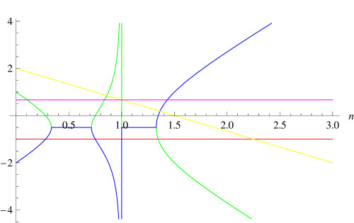
and constitutes the simplest possible example of fourth order gravity. Its homogeneous and isotropic cosmologies have been studied in detail using the dynamical system approach ellisbook ; cdct:dynsys05 ; SanteGenDynSys and the evolution of the large scale cosmological perturbations of a FLRW background has been investigated in SantePert using the covariant gauge invariant approach. The results show some profound differences between this theory and GR. For example, in the transient Friedmann background a=t2n/3(1+w)𝑎superscript𝑡2𝑛31𝑤a=t^{2n/3(1+w)}, ΔmsubscriptΔ𝑚\Delta_{m} was found to grow on long wavelength for almost all the values of the parameter n𝑛n, even when these values corresponded to backgrounds which undergo accelerated expansion (see Figure 1 for a plot of the real part of the exponents of the modes of the ΔmsubscriptΔ𝑚\Delta_{m} solution). In this section we will continue the investigation of the evolution of scalar perturbations for this model 333Clearly we will consider only n>0𝑛0n>0 for this background. Negative values of n𝑛n would represent a contracting model. focusing more specifically on the small scales. Substituting the form of f(R)𝑓𝑅f(R) in the general equations (33-34) we obtain the system (87-88) given in Appendix C.
Refer to caption
Figure 1: Plot against n𝑛n of the real part of the long wavelength modes for Rnsuperscript𝑅𝑛R^{n}-gravity in the dust case (blue, red green and yellow lines) together with the GR modes (red and purple line). This graph is consistent with Figures 2, 3 and 4, i.e., when one of the four perturbation modes grows faster than GR X𝑋X is bigger than zero and when they are all smaller than GR X𝑋X is negative. Of course the cumulative effect of the combination of more than one growing mode has to be taken in account in comparing the two graphs. As one can see this produces a slight shift in the value of n𝑛n associated with the change of sign in X𝑋X and the dominance of one of the Rnsuperscript𝑅𝑛R^{n} growing mode over the GR growing mode.

Providing the details of the background, the values of the parameter n𝑛n, the barotropic factor w𝑤w, the spatial curvature index K𝐾K and the wavenumber k𝑘k one is able to numerically integrate this system to obtain the behaviour of the matter fluctuations. We can then use the quantities described in the previous section to extract physical information about the evolution of density perturbations in this model.

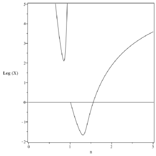
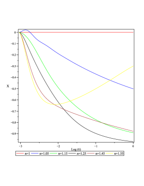
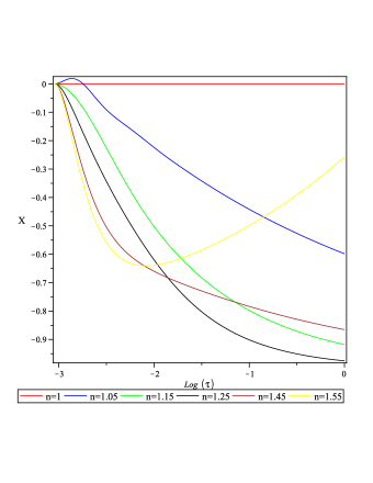
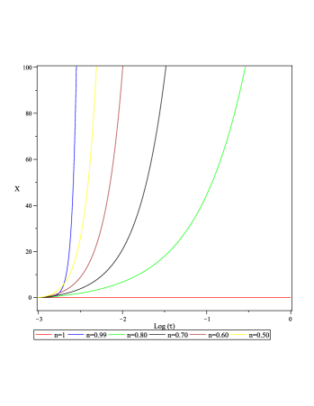
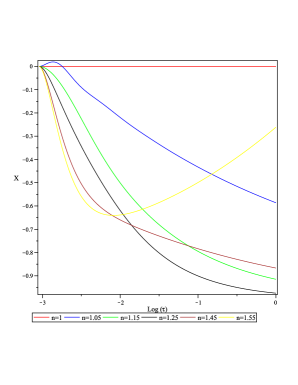
Figure 2 shows the behavior of the quantity X𝑋X as a function of the time parameter τ=log10(S)𝜏subscript10𝑆\tau=\log_{10}(S) on large scales (k0𝑘0k\approx 0) for dust and different values of n𝑛n. If we start with values of n𝑛n close to 1+superscript11^{+} the perturbations seems to first evolve faster than the growing mode of the GR-Einstein-de Sitter case and then at a slower rate which continues to decrease. For higher values of n𝑛n, this first phase is absent and the rate is always slower than in the GR-Einstein-de Sitter case. For n3/2𝑛32n\geq 3/2 the rate of growth of the perturbation is initially below the GR-Einstein-de Sitter mode, however, at late times the mode starts to grow at a much faster rate. For 0<n<10𝑛10<n<1 the situation is radically different: the rate of growth is always faster than GR. As n𝑛n goes from zero to 1superscript11^{-} the growth rate seems to decrease, but at n0.85𝑛0.85n\approx 0.85 this behavior changes and by n=0.90𝑛0.90n=0.90 the perturbations grow much faster than for any other value of n𝑛n. This indicates the possible existence of an instability of the theory in this region of parameter space.
Refer to caption
Refer to caption
Figure 2: Plot of X𝑋X as a function of τ=log10(S)𝜏subscript10𝑆\tau=\log_{10}(S) for Rnsuperscript𝑅𝑛R^{n}-gravity in the long wavelength limit. The red line X=0𝑋0X=0 corresponds to GR. Note the consistency between this picture and Figure 1.
Refer to caption
(a) Plot of log10(X)subscript10𝑋\log_{10}(X) vs n𝑛n at τ=log10(S)=1𝜏subscript10𝑆1\tau=\log_{10}(S)=1
Refer to caption
(b) Plot of Y𝑌Y vs n𝑛n at τ=log10(S)=1𝜏subscript10𝑆1\tau=\log_{10}(S)=1
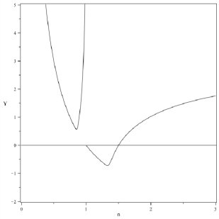
Figure 3: Plots of X𝑋X and Y𝑌Y as a function of n𝑛n evaluated at τ=log10(S)=1𝜏subscript10𝑆1\tau=\log_{10}(S)=1 for Rnsuperscript𝑅𝑛R^{n}-gravity in the long wavelength limit. The horizontal lines X,Y=0𝑋𝑌0X,Y=0 represent the value of these quantities in GR.

These features are well summarized by Figure 3(a) which represents X𝑋X at the present time τ=1𝜏1\tau=1 as function of n𝑛n. When compared with Figure 1 one can see that the two figures are consistent.

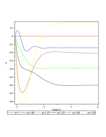
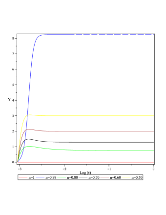
In Figure 4 we see the behavior of Y𝑌Y as a function of τ=log10(S)𝜏subscript10𝑆\tau=\log_{10}(S) for large scale perturbation. It is clear that the growth rate of the perturbations approaches asymptotically a constant value, which corresponds to the dominance of the fastest growing mode of the solutions of the system (87-88). Again, we found consistency between Figure 1 and both this plot and Figure 3(b).
Refer to caption
(a) Plot of Y(τ)𝑌𝜏Y(\tau) for n=1.4𝑛1.4n=1.4
Refer to caption
(b) Plot of Y(τ)𝑌𝜏Y(\tau) for n=1.55𝑛1.55n=1.55
Figure 4: Plot of Y(τ)𝑌𝜏Y(\tau) as a function of τ=log10(S)𝜏subscript10𝑆\tau=\log_{10}(S) for Rnsuperscript𝑅𝑛R^{n}-gravity with n>1𝑛1n>1 (left) and 0<n<10𝑛10<n<1 (right). The red line Y=0𝑌0Y=0 corresponds to GR. Note the consistency between this picture and Figure 1.

This confirms that X𝑋X and Y𝑌Y provide a very useful source of information about the time evolution of scalar perturbations even when we do not have an analytic solution as it often happens in fourth order gravity.

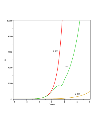
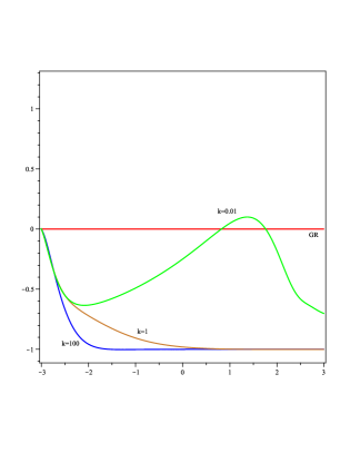
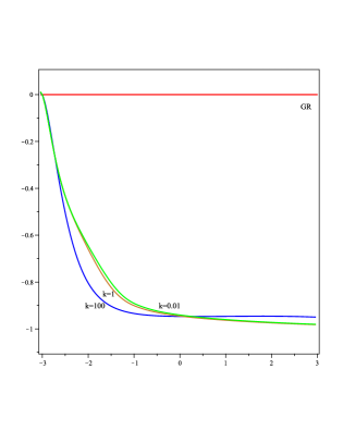
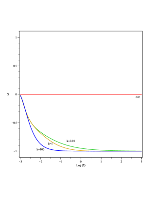
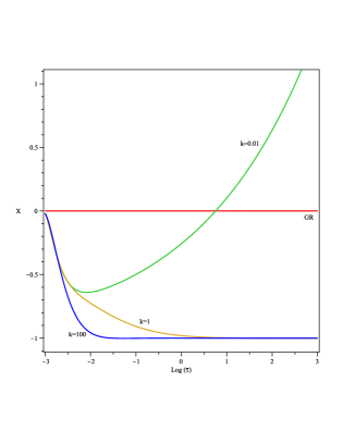
Let us then use the quantity X𝑋X to analyze the growth rate of the matter fluctuation at different scales (see Figure 5). One can see we see that the rate of growth decreases with respect to GR as one tends towards smaller scales. In fact, from the analysis of the time evolution of the power spectrum, we will see that this is associated to a dissipation of the perturbations at that range of scales.
Refer to caption
(a) Plot of X(τ)𝑋𝜏X(\tau) for n=1.4𝑛1.4n=1.4 and different values of k𝑘k
Refer to caption
(b) Plot of X(τ)𝑋𝜏X(\tau) for n=1.55𝑛1.55n=1.55 and different values of k𝑘k
Refer to caption
(c) Plot of X(τ)𝑋𝜏X(\tau) for n=0.9𝑛0.9n=0.9 and different values of k𝑘k
Figure 5: Plot of X(τ)𝑋𝜏X(\tau) as a function of τ=log10(S)𝜏subscript10𝑆\tau=\log_{10}(S) for Rnsuperscript𝑅𝑛R^{n}-gravity and k0𝑘0k\neq 0. Note how the growth of the perturbations is suppressed when k𝑘k grows i.e. when smaller scales are considered.

These results are consistent with the conclusions already drawn in SantePert , i.e. that the dynamics of perturbation growth can be radically different from what happens in GR. This, in turn, implies that the time needed for linear structures to form and, as a consequence, the duration of the matter era, could be very different in this framework. Such features could prove to be an interesting method of placing constraints on the theory of gravity by using data from existing and future large scale structure surveys.

It is also interesting to notice that the behavior of the perturbations for n1𝑛1n\approx 1 is also radically different from the GR case, i.e., even small deviations from n=1𝑛1n=1 are able to produce completely different dynamics. One can understand such behavior since even small deviations from linearity in the action result in a change of order (from two to four) of the perturbation equations, so it is natural to expect significant differences in their solutions.

As already mentioned the equations (33-34) and consequently (87-88) are similar in structure to the equations one would obtain in the classic multi-fluid GR case and these similarities can be used to infer the interaction properties of standard matter and the curvature fluid once the proper variables have been chosen (i.e. ΔmsubscriptΔ𝑚\Delta_{m} and ΔRsubscriptΔ𝑅\Delta_{R} ). The full expressions of these terms in the background given above is too long to be reported in full. However it is instructive to examine their structure. In the ΔmsubscriptΔ𝑚\Delta_{m} equation, the dissipation terms (i.e. the ΔmsubscriptsuperscriptΔ𝑚\Delta^{\prime}_{m} and the ΔRsubscriptsuperscriptΔ𝑅\Delta^{\prime}_{R} terms) are given by

Δm=A1(n,w)t[w+A2(n,w)1+A3(n,w)k2t24n3(1+w)+A3(n,w)(1+A5(n,w)k2t24n3(1+w))1],subscriptsubscriptsuperscriptΔ𝑚subscript𝐴1𝑛𝑤𝑡delimited-[]𝑤subscript𝐴2𝑛𝑤1subscript𝐴3𝑛𝑤superscript𝑘2superscript𝑡24𝑛31𝑤subscript𝐴3𝑛𝑤superscript1subscript𝐴5𝑛𝑤superscript𝑘2superscript𝑡24𝑛31𝑤1{\mathds{C}}_{\Delta^{\prime}_{m}}=\frac{A_{1}(n,w)}{t}\left[w+\frac{A_{2}(n,w)}{1+A_{3}(n,w)k^{2}t^{2-\frac{4n}{3(1+w)}}+A_{3}(n,w)\left(1+A_{5}(n,w)k^{2}t^{2-\frac{4n}{3(1+w)}}\right)^{-1}}\right]\,, (52)

and

ΔR=E1(n,w)t[1+E2(n,w)k2t24n3(1+w)(1+E3(n,w)k2t24n3(1+w))]1,subscriptsubscriptsuperscriptΔ𝑅subscript𝐸1𝑛𝑤𝑡superscriptdelimited-[]1subscript𝐸2𝑛𝑤superscript𝑘2superscript𝑡24𝑛31𝑤1subscript𝐸3𝑛𝑤superscript𝑘2superscript𝑡24𝑛31𝑤1{\mathds{C}}_{\Delta^{\prime}_{R}}=\frac{E_{1}(n,w)}{t}\left[1+E_{2}(n,w)k^{2}t^{2-\frac{4n}{3(1+w)}}(1+E_{3}(n,w)k^{2}t^{2-\frac{4n}{3(1+w)}})\right]^{-1}\,, (53)

respectively, while the source terms are

Δm=B1(n,w)t2[1+B2(n,w)k2t24n3(1+w)(1+B3(n,w)k2t24n3(1+w))1+B4(n,w)k2t24n3(1+w)(1+B5(n,w)k2t24n3(1+w))],subscriptsubscriptΔ𝑚subscript𝐵1𝑛𝑤superscript𝑡2delimited-[]1subscript𝐵2𝑛𝑤superscript𝑘2superscript𝑡24𝑛31𝑤1subscript𝐵3𝑛𝑤superscript𝑘2superscript𝑡24𝑛31𝑤1subscript𝐵4𝑛𝑤superscript𝑘2superscript𝑡24𝑛31𝑤1subscript𝐵5𝑛𝑤superscript𝑘2superscript𝑡24𝑛31𝑤{\mathds{C}}_{\Delta_{m}}=\frac{B_{1}(n,w)}{t^{2}}\left[\frac{1+B_{2}(n,w)k^{2}t^{2-\frac{4n}{3(1+w)}}(1+B_{3}(n,w)k^{2}t^{2-\frac{4n}{3(1+w)}})}{1+B_{4}(n,w)k^{2}t^{2-\frac{4n}{3(1+w)}}(1+B_{5}(n,w)k^{2}t^{2-\frac{4n}{3(1+w)}})}\right]\,, (54)

and

ΔR=C1(n,w)t2[1+C2(n,w)k2t24n3(1+w)(1+C3(n,w)k2t24n3(1+w))1+C4(n,w)k2t24n3(1+w)(1+C5(n,w)k2t24n3(1+w))].subscriptsubscriptΔ𝑅subscript𝐶1𝑛𝑤superscript𝑡2delimited-[]1subscript𝐶2𝑛𝑤superscript𝑘2superscript𝑡24𝑛31𝑤1subscript𝐶3𝑛𝑤superscript𝑘2superscript𝑡24𝑛31𝑤1subscript𝐶4𝑛𝑤superscript𝑘2superscript𝑡24𝑛31𝑤1subscript𝐶5𝑛𝑤superscript𝑘2superscript𝑡24𝑛31𝑤{\mathds{C}}_{\Delta_{R}}=\frac{C_{1}(n,w)}{t^{2}}\left[\frac{1+C_{2}(n,w)k^{2}t^{2-\frac{4n}{3(1+w)}}(1+C_{3}(n,w)k^{2}t^{2-\frac{4n}{3(1+w)}})}{1+C_{4}(n,w)k^{2}t^{2-\frac{4n}{3(1+w)}}(1+C_{5}(n,w)k^{2}t^{2-\frac{4n}{3(1+w)}})}\right]\,. (55)

where Aisubscript𝐴𝑖A_{i}, Bisubscript𝐵𝑖B_{i}, Cisubscript𝐶𝑖C_{i}, Eisubscript𝐸𝑖E_{i} are functions of n𝑛n and w𝑤w only. The structure of the coefficients of ΔRsubscriptsuperscriptΔ𝑅\Delta^{\prime}_{R} is, as expected, similar.

For large scales (k0𝑘0k\rightarrow 0) we have

ΔmA1(n,w)[w+A2(n,w)]t,ΔRE1(n,w)t,ΔmB1(n,w)t2,ΔRC1(n,w)t2,formulae-sequencesubscriptsubscriptsuperscriptΔ𝑚subscript𝐴1𝑛𝑤delimited-[]𝑤subscript𝐴2𝑛𝑤𝑡formulae-sequencesubscriptsubscriptsuperscriptΔ𝑅subscript𝐸1𝑛𝑤𝑡formulae-sequencesubscriptsubscriptΔ𝑚subscript𝐵1𝑛𝑤superscript𝑡2subscriptsubscriptΔ𝑅subscript𝐶1𝑛𝑤superscript𝑡2{\mathds{C}}_{\Delta^{\prime}_{m}}\rightarrow\frac{A_{1}(n,w)\left[w+A_{2}(n,w)\right]}{t}\,,\quad{\mathds{C}}_{\Delta^{\prime}_{R}}\rightarrow\frac{E_{1}(n,w)}{t}\,,\quad{\mathds{C}}_{\Delta_{m}}\rightarrow\frac{B_{1}(n,w)}{t^{2}}\,,\quad{\mathds{C}}_{\Delta_{R}}\rightarrow\frac{C_{1}(n,w)}{t^{2}}\,, (56)

which corresponds to the equations that one would obtain in GR with two collisional fluids. For small scales (k𝑘k\rightarrow\infty) we have

ΔmwA1(n,w)t,ΔR0,ΔmB1(n,w)t2[B3(n,w)B5(n,w)],ΔRC1(n,w)t2[C3(n,w)C5(n,w)],formulae-sequencesubscriptsubscriptsuperscriptΔ𝑚𝑤subscript𝐴1𝑛𝑤𝑡formulae-sequencesubscriptsubscriptsuperscriptΔ𝑅0formulae-sequencesubscriptsubscriptΔ𝑚subscript𝐵1𝑛𝑤superscript𝑡2delimited-[]subscript𝐵3𝑛𝑤subscript𝐵5𝑛𝑤subscriptsubscriptΔ𝑅subscript𝐶1𝑛𝑤superscript𝑡2delimited-[]subscript𝐶3𝑛𝑤subscript𝐶5𝑛𝑤{\mathds{C}}_{\Delta^{\prime}_{m}}\rightarrow w\frac{A_{1}(n,w)}{t}\,,\quad{\mathds{C}}_{\Delta^{\prime}_{R}}\rightarrow 0\,,\quad{\mathds{C}}_{\Delta_{m}}\rightarrow\frac{B_{1}(n,w)}{t^{2}}\left[\frac{B_{3}(n,w)}{B_{5}(n,w)}\right]\,,\quad{\mathds{C}}_{\Delta_{R}}\rightarrow\frac{C_{1}(n,w)}{t^{2}}\left[\frac{C_{3}(n,w)}{C_{5}(n,w)}\right]\;, (57)

which again corresponds to the equations that one would obtains in the case of GR with two fluids, with the difference that this time, since ΔR=0subscriptsubscriptsuperscriptΔ𝑅0{\mathds{C}}_{\Delta^{\prime}_{R}}=0, they are non-collisional 444Note the fact that, in the case of dust (w=0𝑤0w=0) the term ΔmsubscriptsubscriptsuperscriptΔ𝑚{\mathds{C}}_{\Delta^{\prime}_{m}} becomes zero. Although it might appear strange at first sight this is not characteristic of fourth order gravity. In fact the same happens in GR with a mixture of matter and radiation DBE ; Challinor ..

The form of these coefficients is very different to the ones obtained, for example, in the case of a GR baryon-photon system. As we mentioned in this last case the dissipation terms grow as k2superscript𝑘2k^{2}. This means that, as expected, the effect of the interaction between the two fluids becomes more important when one considers smaller scales. In the above case the situation is different because the interaction scale of standard matter and curvature fluid is a non-trivial function of k𝑘k which is peaked at a certain value of k𝑘k. This means that the effect of the interaction is maximized around this specific scale.

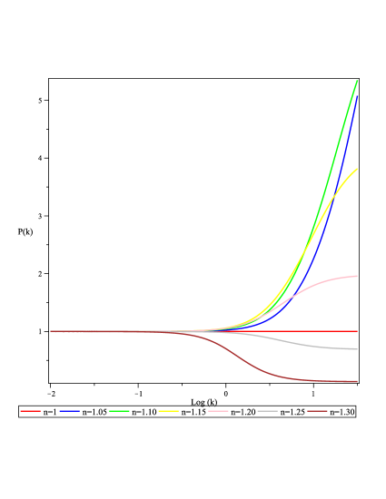
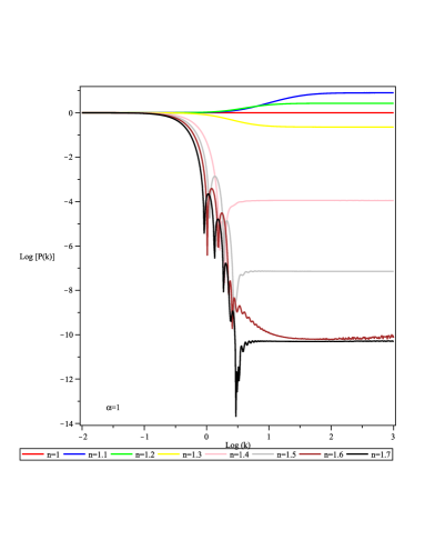
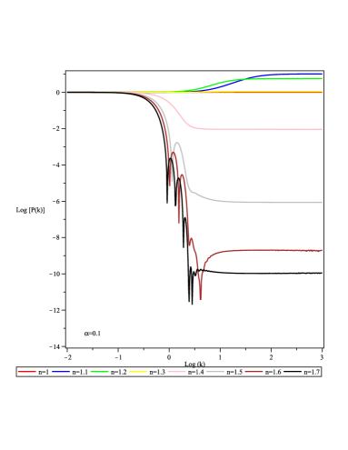
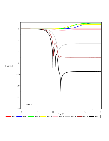
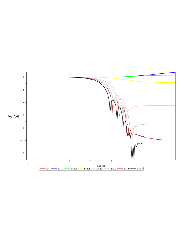
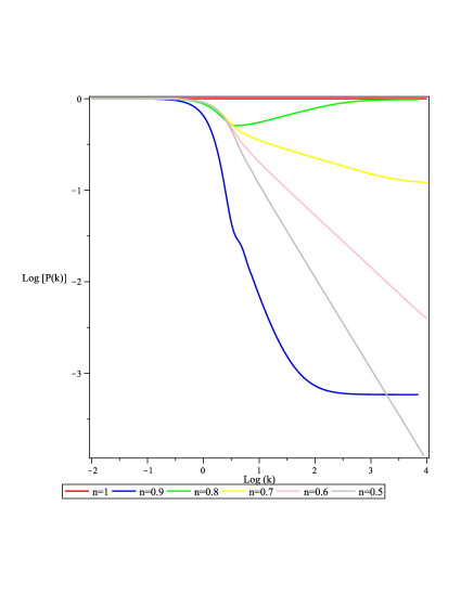
Let us now focus on the impact of these features on the matter power spectrum (Figures 6(a), 6(b), 7). As mentioned in Section IV the k-structure of Equations (33-34) suggest that in fourth order gravity there exist at least three different growth regimes of the perturbations. This is confirmed by our results. In particular, in the case of dust we have three regimes for any values of the remaining parameters: (i) on very large scales the spectrum goes like GR i.e. it is scale invariant; (ii) as k𝑘k becomes bigger the scale invariance is broken and oscillations in the spectrum appear; (iii) for even larger k𝑘k the spectrum becomes again scale invariant. However, on these scales the spectrum can contain either an excess or deficit of power depending on the value of n𝑛n. In particular for n1+𝑛superscript1n\approx 1^{+} small scales have more power than large scales, but, as one moves towards larger values of n𝑛n, the small scale modes are suppressed. For 0<n<10𝑛10<n<1, instead the drop in power seems to decrease as one moves from n=0𝑛0n=0 towards 1superscript11^{-} and we see a sudden increase for n1𝑛superscript1n\approx 1^{-}. It is worth noting the case n0.8𝑛0.8n\approx 0.8 for which there is basically no difference in power between large and small scales and there are no significant oscillations in the spectrum.

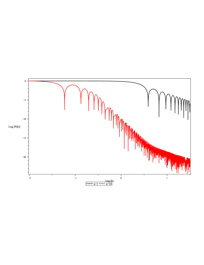
Further indication of the link between the k𝑘k structure of (33-34) and the different regimes of the matter power spectrum can be seen if one analyzes the power spectrum in a radiation dominated era. In this case the perturbations equations contain an additional term which is not present in the dust case. This means that one would expect four different regimes, rather than three. In Figure 8 we have plotted the matter power spectrum of Rnsuperscript𝑅𝑛R^{n}-gravity in the case of radiation and n=10𝑛10n=10 (this value of n𝑛n is chosen only for convenience and it does not have any physical motivation), and as expected one can recognize four different regimes. Note that we obtain the same k𝑘k scaling as in GR on small scales.

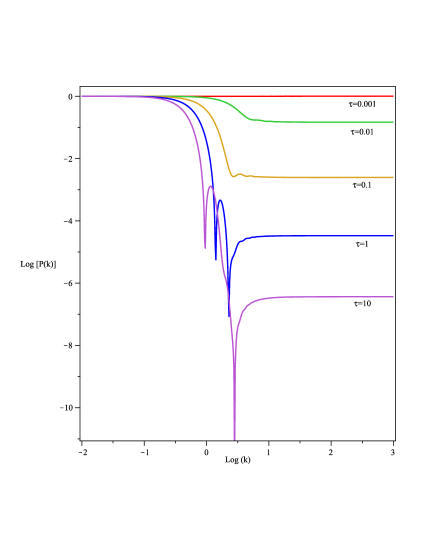
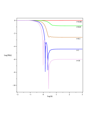
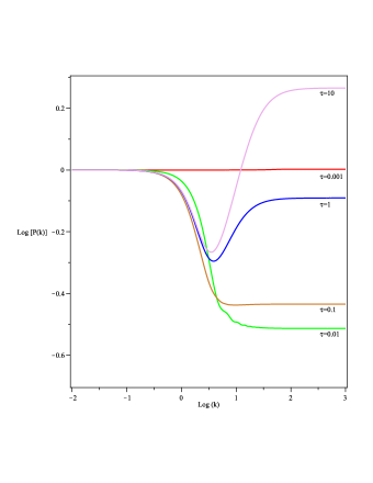
Finally further information on the dynamics of the matter perturbations can be obtained examining the time evolution of the power spectrum. In Figure 9 we give the power spectrum for n=1.4𝑛1.4n=1.4 at different times. One can see that, as the universe expands, the small scale part of the spectrum is more and more suppressed and oscillations start to form. This is in agreement with what one finds from the analysis of X𝑋X and suggests that in this model small scale perturbations tend to be dissipated in time. On the other hand the large scales do not seem to be evolving, which might appear in contrast with what mentioned above. However this is a byproduct of the normalization: for clarity we have normalized the spectrum in such a way that every curve has the same power in long wavelength limit.

The features of the spectrum that we have derived can be then interpreted in terms of the interaction between the curvature fluid and standard matter. On very large and very small scales, the coefficients (52-55) become independent from k𝑘k so that the evolution of the perturbations does not change with the scale and the power spectrum is scale invariant. On intermediate scales the interaction between the two fluids is maximized and the curvature fluid acts as a relativistic component whose pressure is responsible for the oscillations and the dissipation of the small scale perturbations in the same way in which the photons operate in a baryon-photon system 555This suggests the following interesting interpretation for the perturbation variables \mathcal{R} and \Re. These quantities can be thought to represent the modes associated with the contribution of the additional scalar degree of freedom typical of f(R)𝑓𝑅f(R)-gravity. In this sense the spectrum can be explained physically as a consequence of the interaction between these scalar modes and standard matter.. The result is a considerable loss of power for a relatively small variation of the parameter n𝑛n. For example, in the case n=1.4𝑛1.4n=1.4 the difference in power between he two scale invariant parts of the spectrum for n=1.1𝑛1.1n=1.1 is of one order of magnitude while for n=1.6𝑛1.6n=1.6 is about ten orders of magnitude.

Probably the most important consequence of the form of the spectrum presented above is the fact that the effect of these type of fourth order corrections is evident only for a special range of scales, while the rest of the spectrum has the same k𝑘k dependence of GR (but different amplitude). This implies that we have a spectrum that both satisfies the requirement for scale invariance and has distinct features that one could in principle detect, by combining future Cosmic Microwave Background (CMB) and large scale surveys (LSS) Planck ; SDSS .
Refer to caption
(a) Plot of the power spectrum at τ=1𝜏1\tau=1 for Rnsuperscript𝑅𝑛R^{n}-gravity and n>1𝑛1n>1. Note that the spectrum is composed of three parts corresponding to three different evolution regimes for the perturbations.
Refer to caption
(b) Plot of the Power spectrum as a function of k𝑘k for Rnsuperscript𝑅𝑛R^{n}-gravity at τ=1𝜏1\tau=1 and 0<n<10𝑛10<n<1. The spectra for n=0.6𝑛0.6n=0.6 and n=0.5𝑛0.5n=0.5 only approach the scale invariant plateau at extremely high k𝑘k when compared to the other curves. Note the behavior of the spectrum for n0.8𝑛0.8n\approx 0.8, differently from all the other cases, there is basically no loss of power in the spectrum at large k𝑘k.
Figure 6: Power spectra for Rnsuperscript𝑅𝑛R^{n}-gravity
Refer to caption
Figure 7: Detail of the plot of the power spectrum for Rnsuperscript𝑅𝑛R^{n}-gravity at τ=1𝜏1\tau=1. As expected, for these values of n𝑛n we find the presence of the three regimes mentioned in the text. Note also that for n1+𝑛superscript1n\approx 1^{+} the small scales are characterized by an excess of power. Such features is compatible with the results found in Li:2008ai ; HuSawicki ; Bertschinger:2008zb .
Refer to caption
Figure 8: The power spectrum for Rnsuperscript𝑅𝑛R^{n}-gravity at τ=1𝜏1\tau=1 in the case of radiation for GR and Rnsuperscript𝑅𝑛R^{n}-gravity with n=10𝑛10n=10. As expected in this last plot we find four different regimes instead of the three of the dust case: a first regime for k0𝑘0k\rightarrow 0 which is scale invariant; a second and a third regime which correspond to the two different slopes between k102𝑘superscript102k\approx 10^{-2} and k101/2𝑘superscript1012k\approx 10^{1/2} and a fourth regime which has the same slope of the GR plot.
Refer to caption
Figure 9: Evolution the Power spectrum for Rnsuperscript𝑅𝑛R^{n}-gravity for n=1.4𝑛1.4n=1.4. The spectrum has been normalized in such a way that the curves coincide at large scales. Note how, as time passes, small scale perturbations are dissipated and oscillation appear.

VI.2 The case f(R)=R+αRn𝑓𝑅𝑅𝛼superscript𝑅𝑛f(R)=R+\alpha R^{n}

We will now consider a theory with the following action,

L=g[R+αRn+M].𝐿𝑔delimited-[]𝑅𝛼superscript𝑅𝑛subscript𝑀L=\sqrt{-g}\left[R+\alpha R^{n}+{\cal L}_{M}\right]\;. (58)

This theory has gained much popularity as a fourth order gravity model within the context of both inflation and dark energy Ottewill ; star80 ; Suen ; Carroll .

Unlike Rnsuperscript𝑅𝑛R^{n}-gravity, (58) includes explicitly the Hilbert-Einstein term, so that one can consider it as the result of an additive correction to GR. This also means that this model introduces an explicit physical scale which is determined by the relative magnitude of the two terms in the action, making it the simplest fourth order gravity theory with an additional scale for the gravitational interaction.

Some work on estimating the parameter α𝛼\alpha for the specific case of n=2𝑛2n=2 was completed during the eighties. This work was mainly based on arguments pertaining to black hole physics and quantum gravity (see for example Suen ). In the following we will take α𝛼\alpha, which in our units is the ratio between the coupling constant of the fourth order corrections, to be positive definite. Of course, we expect this model to behave much in the same way as the model discussed in the previous section for α𝛼\alpha\rightarrow\infty, and to recover GR for α=0𝛼0\alpha=0. This also means that any new feature in this model will emerge for intermediate values of the coupling.

The f(R)=R+αRn𝑓𝑅𝑅𝛼superscript𝑅𝑛f(R)=R+\alpha R^{n} model has been analyzed at the level of the background using many different approaches (see for example Ottewill ; star80 ; Suen ; Carroll ; Teyssandier:1989dw ), but probably some of the most interesting results for cosmology have been found using the dynamical system approach Barrow Hervik ; SanteGenDynSys ; Amendola:2006kh . The dynamical systems analysis proved that this class of models has, like Rnsuperscript𝑅𝑛R^{n}-gravity, an unstable fixed point associated with the Friedmann-like solution a=t2n/3(1+w)𝑎superscript𝑡2𝑛31𝑤a=t^{2n/3(1+w)}. Substituting the form of the action (58), the system of perturbation equations (33-34) takes the form (97-98) given in Appendix D and one can analyzed the evolution of the scalar perturbations in this background 666Unlike the previous example, the structure of the phase space for this model is not well known. This means that, although in this theory one has a fixed point that resembles the one of Rnsuperscript𝑅𝑛R^{n}-gravity, it is not obvious that it plays the same role. In addition, this background is not, in general, a physical solution of the cosmological equations SanteGenDynSys . This means that there are cosmic histories in which the general integral of these equations approximates the behavior we consider, but it will never be exactly the same. We choose to treat this as a further approximation in our investigation. .

In spite of the fact that both this theory and Rnsuperscript𝑅𝑛R^{n}-gravity have a Friedmann-like solution, dealing with the perturbation equations for this background in f(R)=R+αRn𝑓𝑅𝑅𝛼superscript𝑅𝑛f(R)=R+\alpha R^{n} is considerably more complicated than in Rnsuperscript𝑅𝑛R^{n}-gravity. As a consequence, one is unable to find exact solutions for the perturbation equations, even when one adopts the long wavelength limit. To progress one must numerically integrate the system of perturbation equations and extract useful information relating to the perturbation dynamics using the quantities X𝑋X, Y𝑌Y and the power spectrum.

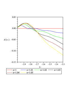
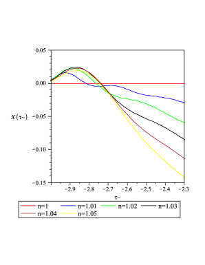
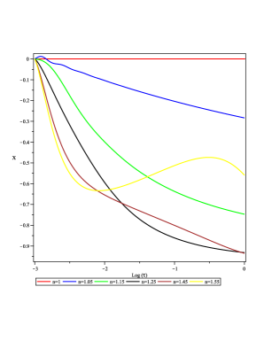
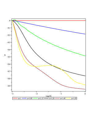
If we look at Figure 10 we notice that for α1𝛼1\alpha\geq 1 the dynamics of the large scale perturbations in this model are similar to those found in Rnsuperscript𝑅𝑛R^{n}-gravity but contain some small differences. For example, from Figure 10(a) one sees that when α=10𝛼10\alpha=10 and n1+𝑛superscript1n\approx 1^{+} the growth rate has some oscillations at small τ𝜏\tau followed by the decay typical of Rnsuperscript𝑅𝑛R^{n}-gravity. However, at smaller values of α𝛼\alpha the situation changes. In particular, the curves that did not show oscillations at small τ𝜏\tau are characterized by the onset of late time oscillations. Because of that the value of n𝑛n at which the growth rate starts to increase at late time is different. These features reveal the important dynamical differences between this model, Rnsuperscript𝑅𝑛R^{n}-gravity and GR. Such differences will be even more evident when we will examine the time evolution of the power spectrum.

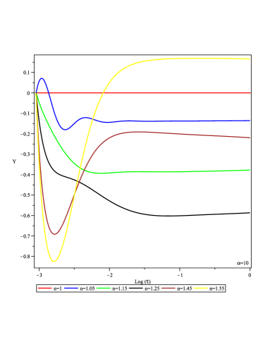
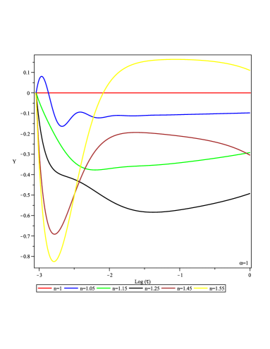
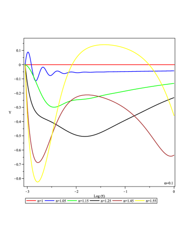
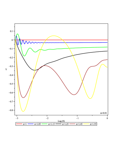
The analysis of the behavior of the quantity Y𝑌Y on large scales also reveal similarities between this model and Rnsuperscript𝑅𝑛R^{n}-gravity. In particular, one sees that, again, for large values of α𝛼\alpha (i.e. α=10)\alpha=10) there is very little difference between the previous example and this model, but when α𝛼\alpha becomes smaller the solution takes more time to saturate and oscillates with a wider amplitude. In addition, the asymptotic values of Y𝑌Y that correspond to the dominant perturbation mode changes with α𝛼\alpha and n𝑛n.

Let us now consider the evolution of the perturbations on smaller scales. The behavior of X𝑋X at different scales (Figures 12) reveals changes in the growth rate. However for different values of α𝛼\alpha and n𝑛n these changes are not always associated with suppression of the growth rate like in the case of Rnsuperscript𝑅𝑛R^{n}-gravity. Figure 12(d) gives an example of these differences.
Refer to caption
(a) Plot of X(τ)𝑋𝜏X(\tau) for f(R)=R+αRn𝑓𝑅𝑅𝛼superscript𝑅𝑛f(R)=R+\alpha R^{n} for large scales (k=0𝑘0k=0), n>1𝑛1n>1, dust and α=10𝛼10\alpha=10. Note the similarity with the plots of Figure 2.
Refer to caption
(b) Plot of X(τ)𝑋𝜏X(\tau) for f(R)=R+αRn𝑓𝑅𝑅𝛼superscript𝑅𝑛f(R)=R+\alpha R^{n} for large scales (k=0𝑘0k=0), n>1𝑛1n>1, dust and α=1𝛼1\alpha=1. Differently from the plot in Figure 10(a) in this case the curve n=1.55𝑛1.55n=1.55 reaches a maximum and then decreases.
Refer to caption
(c) Detail of the plot 10(a) for 1<n<1.051𝑛1.051<n<1.05, The oscillations in the curves are the feature that differentiate f(R)=R+αRn𝑓𝑅𝑅𝛼superscript𝑅𝑛f(R)=R+\alpha R^{n} from Rnsuperscript𝑅𝑛R^{n}-gravity.
Refer to caption
(d) Detail of the plot 10(b) for 1<n<1.051𝑛1.051<n<1.05, The oscillations in the curves are the feature that differentiate f(R)=R+αRn𝑓𝑅𝑅𝛼superscript𝑅𝑛f(R)=R+\alpha R^{n} from Rnsuperscript𝑅𝑛R^{n}-gravity.
Refer to caption
(e) Plot of X(τ)𝑋𝜏X(\tau) for f(R)=R+αRn𝑓𝑅𝑅𝛼superscript𝑅𝑛f(R)=R+\alpha R^{n} for large scales (k=0𝑘0k=0), n>1𝑛1n>1, dust and α=0.1𝛼0.1\alpha=0.1.
Refer to caption
(f) Plot of X(τ)𝑋𝜏X(\tau) for f(R)=R+αRn𝑓𝑅𝑅𝛼superscript𝑅𝑛f(R)=R+\alpha R^{n} for large scales (k=0𝑘0k=0), n>1𝑛1n>1, dust and α=0.01𝛼0.01\alpha=0.01.
Figure 10: Plots of X(τ)𝑋𝜏X(\tau) for large scales in R+αRn𝑅𝛼superscript𝑅𝑛R+\alpha R^{n}-gravity
Refer to caption
(a) Plot of Y(τ)𝑌𝜏Y(\tau) for f(R)=R+αRn𝑓𝑅𝑅𝛼superscript𝑅𝑛f(R)=R+\alpha R^{n} for large scales (k=0𝑘0k=0), n>1𝑛1n>1, dust and α=10𝛼10\alpha=10.
Refer to caption
(b) Plot of Y(τ)𝑌𝜏Y(\tau) for f(R)=R+αRn𝑓𝑅𝑅𝛼superscript𝑅𝑛f(R)=R+\alpha R^{n} for large scales (k=0𝑘0k=0), n>1𝑛1n>1, dust and α=1𝛼1\alpha=1.
Refer to caption
(c) Plot of Y(τ)𝑌𝜏Y(\tau) for f(R)=R+αRn𝑓𝑅𝑅𝛼superscript𝑅𝑛f(R)=R+\alpha R^{n} for large scales (k=0𝑘0k=0), n>1𝑛1n>1, dust and α=0.1𝛼0.1\alpha=0.1
Refer to caption
(d) Plot of Y(τ)𝑌𝜏Y(\tau) for f(R)=R+αRn𝑓𝑅𝑅𝛼superscript𝑅𝑛f(R)=R+\alpha R^{n} for large scales (k=0𝑘0k=0), n>1𝑛1n>1, dust and α=0.01𝛼0.01\alpha=0.01.
Figure 11: Plots of Y(τ)𝑌𝜏Y(\tau) for large scales in R+αRn𝑅𝛼superscript𝑅𝑛R+\alpha R^{n}-gravity
Refer to caption
(a) Plot of X(τ)𝑋𝜏X(\tau) for n=1.4𝑛1.4n=1.4, α=100𝛼100\alpha=100 and various values of k𝑘k
Refer to caption
(b) Plot of X(τ)𝑋𝜏X(\tau) for n=1.4𝑛1.4n=1.4, α=1𝛼1\alpha=1 and various values of k𝑘k
Refer to caption
(c) Plot of X(τ)𝑋𝜏X(\tau) for n=1.4𝑛1.4n=1.4, α=0.01𝛼0.01\alpha=0.01 and various values of k𝑘k
Refer to caption
(d) Plot of X(τ)𝑋𝜏X(\tau) for n=1.55𝑛1.55n=1.55, α=0.01𝛼0.01\alpha=0.01 and various values of k𝑘k
Figure 12: Plot of X(τ)𝑋𝜏X(\tau) as a function of τ=log10(S)𝜏subscript10𝑆\tau=\log_{10}(S) for R+αRn𝑅𝛼superscript𝑅𝑛R+\alpha R^{n}-gravity and k0𝑘0k\neq 0. Note how the growth of the perturbations is suppressed when k𝑘k grows and when α𝛼\alpha decreases.

When one calculates the structure of the coefficients for the ΔmsubscriptΔ𝑚\Delta_{m} equation in the system (Δm,ΔR)subscriptΔ𝑚subscriptΔ𝑅(\Delta_{m},\Delta_{R}) one obtains

Δm=A1(n,w,𝔸)t[w+A2(n,w,𝔸)1+A3(n,w,𝔸)k2t24n3(1+w)+A3(n,w,𝔸)(1+A5(n,w,𝔸)k2t24n3(1+w))1],subscriptsubscriptsuperscriptΔ𝑚subscript𝐴1𝑛𝑤𝔸𝑡delimited-[]𝑤subscript𝐴2𝑛𝑤𝔸1subscript𝐴3𝑛𝑤𝔸superscript𝑘2superscript𝑡24𝑛31𝑤subscript𝐴3𝑛𝑤𝔸superscript1subscript𝐴5𝑛𝑤𝔸superscript𝑘2superscript𝑡24𝑛31𝑤1{\mathds{C}}_{\Delta^{\prime}_{m}}=\frac{A_{1}(n,w,\mathds{A})}{t}\left[w+\frac{A_{2}(n,w,\mathds{A})}{1+A_{3}(n,w,\mathds{A})k^{2}t^{2-\frac{4n}{3(1+w)}}+A_{3}(n,w,\mathds{A})\left(1+A_{5}(n,w,\mathds{A})k^{2}t^{2-\frac{4n}{3(1+w)}}\right)^{-1}}\right]\,, (59)

and

ΔR=E1(n,w,𝔸)t[1+E2(n,w,𝔸)k2t24n3(1+w)(1+E3(n,w,𝔸)k2t24n3(1+w))]1.subscriptsubscriptsuperscriptΔ𝑅subscript𝐸1𝑛𝑤𝔸𝑡superscriptdelimited-[]1subscript𝐸2𝑛𝑤𝔸superscript𝑘2superscript𝑡24𝑛31𝑤1subscript𝐸3𝑛𝑤𝔸superscript𝑘2superscript𝑡24𝑛31𝑤1{\mathds{C}}_{\Delta^{\prime}_{R}}=\frac{E_{1}(n,w,\mathds{A})}{t}\left[1+E_{2}(n,w,\mathds{A})k^{2}t^{2-\frac{4n}{3(1+w)}}(1+E_{3}(n,w,\mathds{A})k^{2}t^{2-\frac{4n}{3(1+w)}})\right]^{-1}\,. (60)

respectively, while the source terms are

Δm=B1(n,w,𝔸)t2[1+B2(n,w,𝔸)k2t24n3(1+w)(1+B3(n,w,𝔸)k2t24n3(1+w))1+B4(n,w,𝔸)k2t24n3(1+w)(1+B5(n,w,𝔸)k2t24n3(1+w))],subscriptsubscriptΔ𝑚subscript𝐵1𝑛𝑤𝔸superscript𝑡2delimited-[]1subscript𝐵2𝑛𝑤𝔸superscript𝑘2superscript𝑡24𝑛31𝑤1subscript𝐵3𝑛𝑤𝔸superscript𝑘2superscript𝑡24𝑛31𝑤1subscript𝐵4𝑛𝑤𝔸superscript𝑘2superscript𝑡24𝑛31𝑤1subscript𝐵5𝑛𝑤𝔸superscript𝑘2superscript𝑡24𝑛31𝑤{\mathds{C}}_{\Delta_{m}}=\frac{B_{1}(n,w,\mathds{A})}{t^{2}}\left[\frac{1+B_{2}(n,w,\mathds{A})k^{2}t^{2-\frac{4n}{3(1+w)}}(1+B_{3}(n,w,\mathds{A})k^{2}t^{2-\frac{4n}{3(1+w)}})}{1+B_{4}(n,w,\mathds{A})k^{2}t^{2-\frac{4n}{3(1+w)}}(1+B_{5}(n,w,\mathds{A})k^{2}t^{2-\frac{4n}{3(1+w)}})}\right]\,, (61)

and

ΔR=C1(n,w,𝔸)t2[1+C2(n,w,𝔸)k2t24n3(1+w)(1+C3(n,w,𝔸)k2t24n3(1+w))1+C4(n,w,𝔸)k2t24n3(1+w)(1+C5(n,w,𝔸)k2t24n3(1+w))],subscriptsubscriptΔ𝑅subscript𝐶1𝑛𝑤𝔸superscript𝑡2delimited-[]1subscript𝐶2𝑛𝑤𝔸superscript𝑘2superscript𝑡24𝑛31𝑤1subscript𝐶3𝑛𝑤𝔸superscript𝑘2superscript𝑡24𝑛31𝑤1subscript𝐶4𝑛𝑤𝔸superscript𝑘2superscript𝑡24𝑛31𝑤1subscript𝐶5𝑛𝑤𝔸superscript𝑘2superscript𝑡24𝑛31𝑤{\mathds{C}}_{\Delta_{R}}=\frac{C_{1}(n,w,\mathds{A})}{t^{2}}\left[\frac{1+C_{2}(n,w,\mathds{A})k^{2}t^{2-\frac{4n}{3(1+w)}}(1+C_{3}(n,w,\mathds{A})k^{2}t^{2-\frac{4n}{3(1+w)}})}{1+C_{4}(n,w,\mathds{A})k^{2}t^{2-\frac{4n}{3(1+w)}}(1+C_{5}(n,w,\mathds{A})k^{2}t^{2-\frac{4n}{3(1+w)}})}\right]\,, (62)

where Aisubscript𝐴𝑖A_{i}, Bisubscript𝐵𝑖B_{i}, Cisubscript𝐶𝑖C_{i}, Eisubscript𝐸𝑖E_{i} are functions of n𝑛n and w𝑤w and 𝔸=αt 2n2𝔸𝛼superscript𝑡2𝑛2\mathds{A}=\alpha\;t^{\,2n-2}. Although the time behavior of these coefficients is always different from GR (unless of course α=0𝛼0\alpha=0), their k𝑘k behavior at a fixed time is similar to the one found in the case f(R)=Rn𝑓𝑅superscript𝑅𝑛f(R)=R^{n}. This means that this model also behaves like a two fluids system for large and small k𝑘k and that the deviation from scale invariance occurs only in a specific k𝑘k interval, which this time is determined by both the parameters α𝛼\alpha and n𝑛n.

These features characterize the spectra shown in Figures 13. As one can clearly see, these plots resemble the ones we have derived in the previous example. There are, of course, differences in the position of the oscillations and the amount of the power drop, but one finds again three different regimes in the case of dust and two of them (k0𝑘0k\rightarrow 0 and k𝑘k\rightarrow\infty ) correspond to scale invariance. Particularly interesting is the fact that in principle the values of α𝛼\alpha and n𝑛n can be fine tuned in such a way to obtain a spectrum in which the small scales have the same power as the large ones. In a situation like this most of the spectrum would be scale invariant and all the deviations would be concentrated around a specific scale.

The time evolution of these spectra also reveals some interesting insight into the dynamics of the matter fluctuations. As usual for large values of α𝛼\alpha the evolution is very similar to the one obtained for Rnsuperscript𝑅𝑛R^{n}-gravity as it is shown in Figure 14(a). However, when the value of the coupling changes the behavior of the perturbations can change dramatically. An example is given in figure 14(b) in which the evolution for the power spectrum of the model (n=1.4,α=00.1)formulae-sequence𝑛1.4𝛼00.1(n=1.4,\alpha=00.1) in which the small scale perturbations are first dissipated and successively start to grow again. This means that in principle one could choose n𝑛n and α𝛼\alpha, such that for example the small scale perturbation grow at different rates at different times. This property could be useful in the resolution of open problems in GR structure formation, like the cosmological dark matter or the excess of red galaxies.

In conclusion, in spite of all the differences in the dynamics of perturbations, the power spectrum in this class of model seems to preserve most of the main structure of the one in Rnsuperscript𝑅𝑛R^{n}-gravity. This implies that all the considerations made in the previous section concerning the physical mechanisms behind the form of the spectrum can be made also in this case. This result was not expected and suggest that we might have encountered a characteristic signature of f(R)𝑓𝑅f(R)-gravity which would be crucial to investigate the validity of these models.
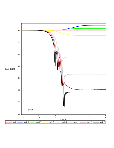
Refer to caption
(a) Plot of P(k)𝑃𝑘P(k) for n>1𝑛1n>1, α=10𝛼10\alpha=10 and various values of k𝑘k
Refer to caption
(b) Plot of P(k)𝑃𝑘P(k) for n>1𝑛1n>1, α=1𝛼1\alpha=1 and various values of k𝑘k
Refer to caption
(c) Plot of P(k)𝑃𝑘P(k) for n>1𝑛1n>1, α=0.1𝛼0.1\alpha=0.1 and various values of k𝑘k
Refer to caption
(d) Plot of P(k)𝑃𝑘P(k) for n>1𝑛1n>1, α=0.01𝛼0.01\alpha=0.01 and various values of k𝑘k
Figure 13: Plot of the Power spectrum as a function of k𝑘k for R+αRn𝑅𝛼superscript𝑅𝑛R+\alpha R^{n}-gravity at τ=1𝜏1\tau=1 for n>1𝑛1n>1.
Refer to caption
(a) Plot of P(k)𝑃𝑘P(k) for n=1.4𝑛1.4n=1.4, α=10𝛼10\alpha=10 and evaluated at various values of τ𝜏\tau
Refer to caption
(b) Plot of P(k)𝑃𝑘P(k) for n=1.4𝑛1.4n=1.4, α=0.01𝛼0.01\alpha=0.01 and evaluated at various values of τ𝜏\tau
Figure 14: The time evolution of the Power spectrum in R+αRn𝑅𝛼superscript𝑅𝑛R+\alpha R^{n}-gravity for n=1.4𝑛1.4n=1.4 and differing values of α𝛼\alpha. Note the drastically differing vertical scales in the plots. Additionally, note the rise in power at small scales at late times in the case of n=1.4𝑛1.4n=1.4 and α=0.01𝛼0.01\alpha=0.01.

VII Discussion and Conclusion

In this paper we have discussed the properties of scalar perturbations in fourth order gravity and described some useful methods for extracting physical information from the complex equations that govern their evolution. These tools are devised in such a way to gain as clear an understanding as possible of the behavior of scalar perturbations on all scales and to facilitate a direct comparison of these results with the corresponding ones in GR. Two simple models: f(R)=Rn𝑓𝑅superscript𝑅𝑛f(R)=R^{n} and f(R)=R+αRn𝑓𝑅𝑅𝛼superscript𝑅𝑛f(R)=R+\alpha R^{n} were analyzed in detail because of their simplicity and because we have a relatively good understanding of their background via the dynamical systems approach.

The results obtained show profound differences in the dynamics of the perturbations compared to what occurs in GR: in these models we find the growth rate of the perturbations is in general different from the GR one and always dependent on the scale. This implies, for example, that depending on the value of the parameters the perturbation can grow or dissipate (or both) at different rates, with obvious consequences for the global cosmic history.

The fourth order system of differential equations that governs the behavior of the scalar perturbations of these models, in particular when written in terms of ΔmsubscriptΔ𝑚\Delta_{m} and ΔRsubscriptΔ𝑅\Delta_{R}, has a structure that resembles closely one of a two fluids GR model. Although the ΔmsubscriptΔ𝑚\Delta_{m} and ΔRsubscriptΔ𝑅\Delta_{R} system of equations is enormously more complicated than (33-34), one can still use it to get an idea of the nature of the interaction between the non-Einstein part of the gravitational interaction and standard matter.

In section VII we found that the wavenumber structure of these coefficients is such that for very large or very small k𝑘k they become scale invariant. This implies, in turn, that the matter power spectrum is scale invariant for k0,𝑘0k\rightarrow 0,\infty and can present some characteristic features on scales that depend on the different parameters of the model. Another way of interpreting the form of the spectrum without necessarily using the curvature fluid idea is to interpret \mathcal{R} and \Re as being associated with the propagation of the scalar degree of freedom of the theory, or a scalar gravitational mode, whose interaction with matter is able to emulate the effect of a relativistic component, which, like photons in GR, induces power loss in the oscillations that appear in the spectrum.

The picture that emerges from our results is that in our examples, fourth order gravity influences deeply the structure formation process, but the modifications are only detectable around a specific value of k𝑘k. Everywhere else in k𝑘k space the results are very close (although dynamically different) to GR. This is particularly interesting since it means that for a suitable choice of values for the parameters, the oscillations can be positioned beyond the observational boundary of currently available data. Hence our results seems to imply that not only could these models be compatible with the observed matter power spectrum, but that we also have a systematic way of constraining their parameters using data coming from a range of scales, for example by combining CMB and LSS data WMAP ; SDSS .

It is also worth commenting briefly about the compatibility of our analysis with the existing literature. For example in Li:2008ai a class of models which is very similar to the one we analyzed in Section VI.2 is considered. Using a specific background the authors showed that the matter power spectrum is characterized by an excess of power at small scales when the theory is very close to ΛΛ\LambdaCDM. A similar result is found in HuSawicki in which classes of models are considered which contain additive corrections to the Hilbert -Einstein action (i.e. they have the form R+g(R)𝑅𝑔𝑅R+g(R) ). These general corrections are parameterized by a quantity B𝐵B, which measures the deviation from GR. Instead in Bertschinger:2008zb , generic modifications are considered (both scale-dependent and scale-independent), using a more flexible parameterization. In the sub-case of scale dependent modifications (like in the f(R)𝑓𝑅f(R) case) examples are given in which one finds once again excess of power on small scales in the power spectrum. Also one should note that in the same sub-case examples were given when one finds a deficit in power.

Interestingly, both the examples considered in this paper exhibit excess power on small scales for n1+𝑛superscript1n\rightarrow 1^{+} in the case of Rnsuperscript𝑅𝑛R^{n}-gravity and for n1+𝑛superscript1n\rightarrow 1^{+} and α1much-less-than𝛼1\alpha\ll 1 in the case R+αRn𝑅𝛼superscript𝑅𝑛R+\alpha R^{n}. This indicates that, for small corrections to GR, excess power at large scale seems to be a generic feature in f(R)𝑓𝑅f(R)-gravity. However there are situations in which one might want to analyze theories which are not necessarily close to GR. For example in Salv06 ; Salv07 ; Salucci a fit of Rnsuperscript𝑅𝑛R^{n}-gravity with the data coming from the rotation curves of galaxies and supernovae type Ia leads to values of n𝑛n in the range [1.7,3.5]1.73.5[1.7,3.5]. For these values of n𝑛n, both our examples indicate a loss of power at small scales, which means that we are provided with an opportunity to rule out this model by testing it against available data. Although the presence of an excess or deficit of power on small scales seems closely related to the value of the specific parameters of the model itself, there are some indications that other features of the spectrum found in our examples are indeed general. For example, the k𝑘k structure of the general equations (40-41) suggests that the evolution of perturbations in a generic f(R)𝑓𝑅f(R) theory presents at least three different regimes. Also looking at the derivation of the (Δm,ΔR)subscriptΔ𝑚subscriptΔ𝑅(\Delta_{m},\Delta_{R}) equations (which can be performed in general, provided a sufficiently large amount of paper and time) one realizes that the k𝑘k dependence of the dissipation and source coefficients we have found in our examples is expected to be common to any f(R)𝑓𝑅f(R) Lagrangian because it originates from the ~2~2superscript~2superscript~2\tilde{\nabla}^{2}\tilde{\nabla}^{2} terms in the perturbation equations.

We end by commenting that these results together with the dynamical systems analysis of the background cosmological history presented in other papers OurDynSys ; SanteGenDynSys provides a unified and consistent approach to the combined study of FLRW observational constraints and a complete analysis of linear structure growth in the context of f(R)𝑓𝑅f(R) gravity.

Acknowledgements:
The authors wish to thank Dr J. Larena for useful discussion and suggestions. SC wish to thanks J Donkers for useful discussion and support during the development of this paper. KNA and SC are supported by Claude Leon Foundation fellowships. This work was supported by the National Research Foundation (South Africa) and the Ministrero degli Affari Esteri - DIG per la Promozione e Cooperazione Culturale (Italy) under the joint Italy/South Africa science and technology agreement.

Appendix A General propagation and constraint equations of the 1+3 covariant formalism.

Expansion propagation (generalized Raychaudhuri equation):

Θ˙+13Θ2+σabσab2ωaωa~au˙a+u˙au˙a+12(μ~m+3p~m)=12(μR+3pR).˙Θ13superscriptΘ2subscript𝜎𝑎𝑏superscript𝜎𝑎𝑏2subscript𝜔𝑎superscript𝜔𝑎superscript~𝑎subscript˙𝑢𝑎subscript˙𝑢𝑎superscript˙𝑢𝑎12superscript~𝜇𝑚3superscript~𝑝𝑚12superscript𝜇𝑅3superscript𝑝𝑅\displaystyle\dot{\Theta}+{\textstyle\frac{1}{3}}\Theta^{2}+\sigma_{{{a}}{{b}}}\sigma^{{{a}}{{b}}}-2\omega_{{a}}\omega^{{a}}-\tilde{\nabla}^{a}\dot{u}_{{a}}+\dot{u}_{{a}}\dot{u}^{{a}}+{\textstyle\frac{1}{2}}(\tilde{\mu}^{m}+3\tilde{p}^{m})=-{\textstyle\frac{1}{2}}({\mu}^{R}+3{p}^{R})\;. (63)

Vorticity propagation:

ω˙a+23Θωa+12curlu˙aσabωb=0.subscript˙𝜔delimited-⟨⟩𝑎23Θsubscript𝜔𝑎12curlsubscript˙𝑢𝑎subscript𝜎𝑎𝑏superscript𝜔𝑏0\dot{\omega}_{\langle{{a}}\rangle}+{\textstyle\frac{2}{3}}\Theta\omega_{{a}}+{\textstyle\frac{1}{2}}\mbox{curl}\,\dot{u}_{{a}}-\sigma_{{{a}}{{b}}}\omega^{{b}}=0\;. (64)

Shear propagation:

σ˙ab+23Θσab+Eab~au˙b+σcaσb+cωaωbu˙au˙b=12πabR.\dot{\sigma}_{\langle{{a}}{{b}}\rangle}+{\textstyle\frac{2}{3}}\Theta\sigma_{{{a}}{{b}}}+E_{{{a}}{{b}}}-\tilde{\nabla}_{\langle{{a}}}\dot{u}_{{{b}}\rangle}+\sigma_{{c}\langle{{a}}}\sigma_{{{b}}\rangle}{}^{c}+\omega_{\langle{{a}}}\omega_{{{b}}\rangle}-\dot{u}_{\langle{{a}}}\dot{u}_{{{b}}\rangle}\,=\,{\textstyle\frac{1}{2}}\pi^{R}_{{{a}}{{b}}}\;. (65)

Gravito-electric propagation:

E˙ab+ΘEabcurlHab+12(μ~m+p~m)σab2u˙cεcd(aHb)d3σcaEb+cωcεcd(aEb)d\displaystyle\dot{E}_{\langle{{a}}{{b}}\rangle}+\Theta E_{{{a}}{{b}}}-\mbox{curl}\,H_{{{a}}{{b}}}+{\textstyle\frac{1}{2}}(\tilde{\mu}^{m}+\tilde{p}^{m})\sigma_{{{a}}{{b}}}-2\dot{u}^{c}\varepsilon_{{c}{d}({{a}}}H_{{{b}})}{}^{d}-3\sigma_{{c}\langle{{a}}}E_{{{b}}\rangle}{}^{c}+\omega^{c}\varepsilon_{{c}{d}({{a}}}E_{{{b}})}{}^{d}
=12(μR+pR)σab12π˙abR12~aqbR16ΘπabR12σcπbcRa12ωcεc(adπb)dR.\displaystyle~{}~{}{}=-{\textstyle\frac{1}{2}}(\mu^{R}+p^{R})\sigma_{{{a}}{{b}}}-{\textstyle\frac{1}{2}}\dot{\pi}^{R}_{\langle{{a}}{{b}}\rangle}-{\textstyle\frac{1}{2}}\tilde{\nabla}_{\langle{{a}}}q^{R}_{{{b}}\rangle}-{\textstyle\frac{1}{6}}\Theta\pi^{R}_{{{a}}{{b}}}-{\textstyle\frac{1}{2}}\sigma^{c}{}_{\langle{{a}}}\pi^{R}_{{{b}}\rangle{c}}-{\textstyle\frac{1}{2}}\omega^{c}\varepsilon_{{c}({{a}}}^{d}\pi^{R}_{b)d}\;. (66)

Gravito-magnetic propagation:

H˙ab+ΘHab+curlEab3σcaHb+cωcεcd(aHb)+d2u˙cεcd(aEb)d\displaystyle\dot{H}_{\langle{{a}}{{b}}\rangle}+\Theta H_{{{a}}{{b}}}+\mbox{curl}\,E_{{{a}}{{b}}}-3\sigma_{{c}\langle{{a}}}H_{{{b}}\rangle}{}^{c}+\omega^{c}\varepsilon_{{c}{d}({{a}}}H_{{{b}})}{}^{d}+2\dot{u}^{c}\varepsilon_{{c}{d}({{a}}}E_{{{b}})}{}^{d}
=12curlπabR32ωaqbR+12σcεb)cd(aqdR.\displaystyle~{}~{}{}={\textstyle\frac{1}{2}}\mbox{curl}\,\pi^{R}_{{{a}}{{b}}}-{\textstyle\frac{3}{2}}\omega_{\langle{{a}}}q^{R}_{{{b}}\rangle}+{\textstyle\frac{1}{2}}\sigma^{c}{}_{({{a}}}\varepsilon_{{{b}}){c}}^{\;\;\;\;d}q^{R}_{d}\;. (67)

Vorticity constraint:

~aωau˙aωa=0.superscript~𝑎subscript𝜔𝑎superscript˙𝑢𝑎subscript𝜔𝑎0\tilde{\nabla}^{{a}}\omega_{{a}}-\dot{u}^{{a}}\omega_{{a}}=0\;. (68)

Shear constraint:

~bσabcurlωa23~aΘ+2[ω,u˙]a=qaR.superscript~𝑏subscript𝜎𝑎𝑏curlsubscript𝜔𝑎23subscript~𝑎Θ2subscript𝜔˙𝑢𝑎subscriptsuperscript𝑞𝑅𝑎\tilde{\nabla}^{{b}}\sigma_{{{a}}{{b}}}-\mbox{curl}\,\omega_{{a}}-{\textstyle\frac{2}{3}}\tilde{\nabla}_{{a}}\Theta+2[\omega,\dot{u}]_{{a}}=-q^{R}_{a}\;. (69)

Gravito-magnetic constraint:

curlσab+~aωbHab+2u˙aωb=0.\mbox{curl}\,\sigma_{{{a}}{{b}}}+\tilde{\nabla}_{\langle{{a}}}\omega_{{{b}}\rangle}-H_{{{a}}{{b}}}+2\dot{u}_{\langle{{a}}}\omega_{{{b}}\rangle}=0\;. (70)

Gravito-electric divergence:

~bEab13~aμ~m[σ,H]a+3Habωb=12σabqbR32[ω,qR]a12~bπabR+13~aμR13ΘqaR.superscript~𝑏subscript𝐸𝑎𝑏13subscript~𝑎superscript~𝜇𝑚subscript𝜎𝐻𝑎3subscript𝐻𝑎𝑏superscript𝜔𝑏12superscriptsubscript𝜎𝑎𝑏subscriptsuperscript𝑞𝑅𝑏32subscript𝜔superscript𝑞𝑅𝑎12superscript~𝑏subscriptsuperscript𝜋𝑅𝑎𝑏13subscript~𝑎superscript𝜇𝑅13Θsubscriptsuperscript𝑞𝑅𝑎\displaystyle\tilde{\nabla}^{{b}}E_{{{a}}{{b}}}-{\textstyle\frac{1}{3}}\tilde{\nabla}_{{a}}\tilde{\mu}^{m}-[\sigma,H]_{{a}}+3H_{{{a}}{{b}}}\omega^{{b}}={\textstyle\frac{1}{2}}\sigma_{{{a}}}^{{b}}q^{R}_{{b}}-{\textstyle\frac{3}{2}}[\omega,q^{R}]_{{a}}-{\textstyle\frac{1}{2}}\tilde{\nabla}^{{b}}\pi^{R}_{{{a}}{{b}}}+{\textstyle\frac{1}{3}}\tilde{\nabla}_{{a}}\mu^{R}-{\textstyle\frac{1}{3}}\Theta q^{R}_{{a}}\;. (71)

Gravito-magnetic divergence:

~bHab(μ~m+p~m)ωa+[σ,E]a3Eabωb=12curlqaR+(μR+pR)ωa12[σ,πR]a12πabRωb.superscript~𝑏subscript𝐻𝑎𝑏superscript~𝜇𝑚superscript~𝑝𝑚subscript𝜔𝑎subscript𝜎𝐸𝑎3subscript𝐸𝑎𝑏superscript𝜔𝑏12curlsubscriptsuperscript𝑞𝑅𝑎superscript𝜇𝑅superscript𝑝𝑅subscript𝜔𝑎12subscript𝜎superscript𝜋𝑅𝑎12subscriptsuperscript𝜋𝑅𝑎𝑏superscript𝜔𝑏\displaystyle\tilde{\nabla}^{{b}}H_{{{a}}{{b}}}-(\tilde{\mu}^{m}+\tilde{p}^{m})\omega_{{a}}+[\sigma,E]_{{a}}-3E_{{{a}}{{b}}}\omega^{{b}}=-{\textstyle\frac{1}{2}}\mbox{curl}\,q^{R}_{{a}}+(\mu^{R}+p^{R})\omega_{{a}}-{\textstyle\frac{1}{2}}[\sigma,\pi^{R}]_{{a}}-{\textstyle\frac{1}{2}}\pi^{R}_{{{a}}{{b}}}\omega^{{b}}\;. (72)

Standard Matter Conservation

μ˙m=Θ(μm+pm),superscript˙𝜇𝑚Θsuperscript𝜇𝑚superscript𝑝𝑚\displaystyle\dot{\mu}^{m}\,=\,-\,\Theta\,(\mu^{m}+{p^{m}})\;, (73)
~apm=(μm+pm)u˙a.superscript~𝑎superscript𝑝𝑚superscript𝜇𝑚superscript𝑝𝑚superscript˙𝑢𝑎\displaystyle\tilde{\nabla}^{a}{p^{m}}=-(\mu^{m}+{p^{m}})\,\dot{u}^{a}\,. (74)

Curvature fluid Conservation

μR˙+~aqaR=Θ(μR+pR)2(u˙aqaR)(σaπbRb)a+μmf′′R˙f2,\displaystyle\dot{\mu^{R}}+\tilde{\nabla}^{a}q^{R}_{a}=-\,\Theta\,(\mu^{R}+p^{R})-2\,(\dot{u}^{a}q^{R}_{a})-(\sigma^{a}\!{}^{b}\pi^{R}_{b}\!{}_{a})+\mu^{m}\frac{f^{\prime\prime}\,\dot{R}}{f^{\prime 2}}\;, (75)
q˙aR+~apR+~bπabR=43ΘqaRσabqbR(μR+pR)u˙au˙bπabRηabcωbqcR+μmf′′~aRf2subscriptsuperscript˙𝑞𝑅delimited-⟨⟩𝑎subscript~𝑎superscript𝑝𝑅superscript~𝑏subscriptsuperscript𝜋𝑅𝑎𝑏43Θsubscriptsuperscript𝑞𝑅𝑎superscriptsubscript𝜎𝑎𝑏subscriptsuperscript𝑞𝑅𝑏superscript𝜇𝑅superscript𝑝𝑅subscript˙𝑢𝑎superscript˙𝑢𝑏subscriptsuperscript𝜋𝑅𝑎𝑏superscriptsubscript𝜂𝑎𝑏𝑐subscript𝜔𝑏subscriptsuperscript𝑞𝑅𝑐superscript𝜇𝑚superscript𝑓′′subscript~𝑎𝑅superscript𝑓2\displaystyle\dot{q}^{R}_{\langle a\rangle}+\tilde{\nabla}_{a}p^{R}+\tilde{\nabla}^{b}\pi^{R}_{ab}=-\,{\textstyle\frac{4}{3}}\,\Theta\,q^{R}_{a}-\sigma_{a}\!^{b}\,q^{R}_{b}-(\mu^{R}+p^{R})\,\dot{u}_{a}-\dot{u}^{b}\,\pi^{R}_{ab}-\eta_{a}^{bc}\,\omega_{b}\,q^{R}_{c}+\mu^{m}\frac{f^{\prime\prime}\,\tilde{\nabla}_{a}{R}}{f^{\prime 2}}\ (76)

As usual angle brackets applied to a vector denote the projection of this vector on the tangent 3-spaces

Va=haVbb.subscript𝑉delimited-⟨⟩𝑎subscript𝑎superscriptsubscript𝑉𝑏𝑏V_{\langle{{a}}\rangle}=h_{{a}}{}^{{b}}V_{{b}}\;. (77)

Instead when applied to a tensor they denote the projected, symmetric and trace free part of this object

Wab=[h(ahb)cd13hcdhab]Wcd.W_{\langle{{a}}{{b}}\rangle}=\left[h_{({{a}}}{}^{c}h_{{{b}})}{}^{d}-{\textstyle\frac{1}{3}}h^{{c}{d}}h_{{{a}}{{b}}}\right]W_{{c}{d}}\,. (78)

The spatial curl of a vector and a tensor is

(curlX)a=ϵabc~bXc(curlX)ab=ϵcda~cXdb(\mbox{curl}\,X)^{a}=\epsilon^{abc}\,\tilde{\nabla}_{b}X_{c}\qquad\qquad(\mbox{curl}\,X)^{ab}=\epsilon^{cd\langle a}\,\tilde{\nabla}_{c}X^{b\rangle}\!_{d} (79)

respectively, where ϵabc=udηabcdsubscriptitalic-ϵ𝑎𝑏𝑐superscript𝑢𝑑subscript𝜂𝑎𝑏𝑐𝑑\epsilon_{abc}=u^{d}\eta_{abcd} is the spatial volume. Finally ωa=12εaωbcbcsubscript𝜔𝑎12subscript𝜀𝑎superscriptsubscript𝜔𝑏𝑐𝑏𝑐\omega_{{a}}=\frac{1}{2}\varepsilon_{a}{}^{{b}{c}}\omega_{bc} and the covariant tensor commutator is

[W,Z]a=εacdWcZdee.subscript𝑊𝑍𝑎subscript𝜀𝑎𝑐𝑑superscript𝑊𝑐subscriptsuperscript𝑍𝑑𝑒𝑒[W,Z]_{{a}}=\varepsilon_{{{a}}{c}{d}}W^{c}{}_{e}Z^{{d}{e}}\,.

The 1+3 equations above are completely equivalent to the Einstein equation and govern the dynamics of the matter and gravitational fields in fourth order gravity. As we will see the new source terms in their R.H.S. will modify the evolution of the perturbations in a non-trivial way. The standard GR equations are obtained by setting f(R)=R𝑓𝑅𝑅f(R)=R which corresponds to setting all these sources to zero.

Appendix B The Covariant Gauge Invariant gradient equations

In the following we give, for completeness, the equations for the evolution of the gradient variables

𝒟am=Sμm~aμm,Za=S~aΘ,Ca=S~aR~,a=S~aR,a=S~aR˙.formulae-sequencesubscriptsuperscript𝒟𝑚𝑎𝑆superscript𝜇𝑚subscript~𝑎superscript𝜇𝑚formulae-sequencesubscript𝑍𝑎𝑆subscript~𝑎Θformulae-sequencesubscript𝐶𝑎𝑆subscript~𝑎~𝑅formulae-sequencesubscript𝑎𝑆subscript~𝑎𝑅subscript𝑎𝑆subscript~𝑎˙𝑅{\cal D}^{m}_{{a}}=\frac{S}{\mu^{m}}\tilde{\nabla}_{{a}}\mu^{m}\,,\qquad Z_{{a}}=S\tilde{\nabla}_{{a}}\Theta\,,\qquad C_{{a}}=S\tilde{\nabla}_{{a}}\tilde{R}\;,\qquad{\cal R}_{{a}}=S\tilde{\nabla}_{{a}}R\,,\qquad\Re_{a}=S\tilde{\nabla}_{{a}}\dot{R}\;. (80)

They read

𝒟˙amsubscriptsuperscript˙𝒟𝑚𝑎\displaystyle\dot{{\cal D}}^{m}_{{a}} =\displaystyle= wΘ𝒟am(1+w)Za,𝑤Θsubscriptsuperscript𝒟𝑚𝑎1𝑤subscript𝑍𝑎\displaystyle w\Theta{\cal D}^{m}_{{a}}-(1+w)Z_{{a}}\,, (81)
Z˙asubscript˙𝑍𝑎\displaystyle\dot{Z}_{{a}} =\displaystyle= (R˙f′′f2Θ3)Za+[3(w1)(3w+2)6(w+1)μf+2wΘ2+3w(μR+3pR)6(w+1)+2ww+1kS2]𝒟am+Θf′′2fa˙𝑅superscript𝑓′′superscript𝑓2Θ3subscript𝑍𝑎delimited-[]3𝑤13𝑤26𝑤1𝜇superscript𝑓2𝑤superscriptΘ23𝑤superscript𝜇𝑅3superscript𝑝𝑅6𝑤12𝑤𝑤1𝑘superscript𝑆2subscriptsuperscript𝒟𝑚𝑎Θsuperscript𝑓′′2superscript𝑓subscript𝑎\displaystyle\left(\frac{\dot{R}f^{\prime\prime}}{f^{\prime}}-\frac{2\Theta}{3}\right)Z_{a}+\left[\frac{3(w-1)(3w+2)}{6(w+1)}\frac{\mu}{f^{\prime}}+\frac{2w\Theta^{2}+3w(\mu^{R}+3p^{R})}{6(w+1)}+\frac{2w}{w+1}\frac{k}{S^{2}}\right]{\cal D}^{m}_{a}+\frac{\Theta f^{\prime\prime}}{2f^{\prime}}\Re_{a} (82)
+[12+2f′′fkS212fff′′f+f′′fμf+R˙Θ(f′′f)2+R˙Θf(3)f]aww+1~2𝒟amf′′f~2a,delimited-[]122superscript𝑓′′superscript𝑓𝑘superscript𝑆212𝑓superscript𝑓superscript𝑓′′superscript𝑓superscript𝑓′′superscript𝑓𝜇superscript𝑓˙𝑅Θsuperscriptsuperscript𝑓′′superscript𝑓2˙𝑅Θsuperscript𝑓3superscript𝑓subscript𝑎𝑤𝑤1superscript~2subscriptsuperscript𝒟𝑚𝑎superscript𝑓′′superscript𝑓superscript~2subscript𝑎\displaystyle+\left[\frac{1}{2}+2\frac{f^{\prime\prime}}{f^{\prime}}\frac{k}{S^{2}}-\frac{1}{2}\frac{f}{f^{\prime}}\frac{f^{\prime\prime}}{f^{\prime}}+\frac{f^{\prime\prime}}{f^{\prime}}\frac{\mu}{f^{\prime}}+\dot{R}\Theta\left(\frac{f^{\prime\prime}}{f^{\prime}}\right)^{2}+\dot{R}\Theta\frac{f^{(3)}}{f^{\prime}}\right]\mathcal{R}_{a}-\frac{w}{w+1}\tilde{\nabla}^{2}{\cal D}^{m}_{a}-\frac{f^{\prime\prime}}{f^{\prime}}\tilde{\nabla}^{2}\mathcal{R}_{a}\,,
˙asubscript˙𝑎\displaystyle\dot{{\cal R}}_{a} =\displaystyle= aww+1R˙𝒟am,subscript𝑎𝑤𝑤1˙𝑅subscriptsuperscript𝒟𝑚𝑎\displaystyle\Re_{a}-\frac{w}{w+1}\dot{R}\;{\cal D}^{m}_{{a}}\,, (83)
˙asubscript˙𝑎\displaystyle\dot{\Re}_{a} =\displaystyle= (Θ+2R˙f(3)f′′)aR˙Za[(3w1)3μf′′+3ww+1(pR+μR)ff′′+w3(w+1)R˙(Θ3R˙f(3)f′′)]𝒟amΘ2˙𝑅superscript𝑓3superscript𝑓′′subscript𝑎˙𝑅subscript𝑍𝑎delimited-[]3𝑤13𝜇superscript𝑓′′3𝑤𝑤1superscript𝑝𝑅superscript𝜇𝑅superscript𝑓superscript𝑓′′𝑤3𝑤1˙𝑅Θ3˙𝑅superscript𝑓3superscript𝑓′′subscriptsuperscript𝒟𝑚𝑎\displaystyle-\left(\Theta+2\dot{R}\frac{f^{(3)}}{f^{\prime\prime}}\right)\Re_{a}-\dot{R}Z_{a}-\left[\frac{(3w-1)}{3}\frac{\mu}{f^{\prime\prime}}+3\frac{w}{w+1}(p^{R}+\mu^{R})\frac{f^{\prime}}{f^{\prime\prime}}+\frac{w}{3(w+1)}\dot{R}\left(\Theta-3\dot{R}\frac{f^{(3)}}{f^{\prime\prime}}\right)\right]{\cal D}^{m}_{{a}} (84)
+[32(1+w)kS2(13ff′′+f(4)fR˙2+Θf(3)fR˙29Θ2+13(μR+3pR)+R¨f(3)f′′\displaystyle+\left[\frac{3}{2}(1+w)\frac{k}{S^{2}}-\left(\frac{1}{3}\frac{f^{\prime}}{f^{\prime\prime}}+\frac{f^{(4)}}{f^{\prime}}\dot{R}^{2}+\Theta\frac{f^{(3)}}{f^{\prime}}\dot{R}-\frac{2}{9}\Theta^{2}+\frac{1}{3}(\mu^{R}+3p^{R})+\ddot{R}\frac{f^{(3)}}{f^{\prime\prime}}\right.\right.
16ff+12(w+1)μf13R˙Θf′′f)]a+~2a,\displaystyle\left.\left.-\frac{1}{6}\frac{f}{f^{\prime}}+\frac{1}{2}(w+1)\frac{\mu}{f^{\prime}}-\frac{1}{3}\dot{R}\Theta\frac{f^{\prime\prime}}{f^{\prime}}\right)\right]\mathcal{R}_{a}+\tilde{\nabla}^{2}\mathcal{R}_{a}\,,

together with the constraint

CaS2+(43Θ+2R˙f′′f)Za2μf𝒟am+[2R˙Θf(3)ff′′f2(f2μ+2R˙Θf′′4kS2)]a+2Θf′′fa2f′′f~2a=0.subscript𝐶𝑎superscript𝑆243Θ2˙𝑅superscript𝑓′′superscript𝑓subscript𝑍𝑎2𝜇superscript𝑓subscriptsuperscript𝒟𝑚𝑎delimited-[]2˙𝑅Θsuperscript𝑓3superscript𝑓superscript𝑓′′superscript𝑓2𝑓2𝜇2˙𝑅Θsuperscript𝑓′′4𝑘superscript𝑆2subscript𝑎2Θsuperscript𝑓′′superscript𝑓subscript𝑎2superscript𝑓′′superscript𝑓superscript~2subscript𝑎0\frac{C_{a}}{S^{2}}+\left(\frac{4}{3}\Theta+\frac{2\dot{R}f^{\prime\prime}}{f^{\prime}}\right)Z_{a}-2\frac{\mu}{f^{\prime}}{\cal D}^{m}_{{a}}+\left[2\dot{R}\Theta\frac{f^{(3)}}{f^{\prime}}-\frac{f^{\prime\prime}}{f^{\prime 2}}\left(f-2\mu+2\dot{R}\Theta f^{\prime\prime}-4\frac{k}{S^{2}}\right)\right]\mathcal{R}_{a}+\frac{2\Theta f^{\prime\prime}}{f^{\prime}}\Re_{a}-\frac{2f^{\prime\prime}}{f^{\prime}}\tilde{\nabla}^{2}\mathcal{R}_{a}=0\,. (85)

The propagation equation for the variable C is

C˙a=6k2S2Θ(5f′′fa3𝒟am)+k{3S2ΘCa+(6μRΘ2(3ω)Θ3(ω+1))𝒟am6f′′Θf~2a\displaystyle\dot{C}_{a}=\frac{6k^{2}}{S^{2}\Theta}\left(5\frac{f^{\prime\prime}}{f^{\prime}}\mathcal{R}_{a}-3\mathcal{D}^{m}_{a}\right)+k\left\{\frac{3}{S^{2}\Theta}C_{a}+\left(\frac{6\mu^{R}}{\Theta}-\frac{2(3\omega)\Theta}{3(\omega+1)}\right)\mathcal{D}^{m}_{a}-\frac{6f^{\prime\prime}}{\Theta f^{\prime}}\tilde{\nabla}^{2}\mathcal{R}_{a}\right.
+[6Rf′′2f2+(2(Θ23μR)f3f)f′′Θf2+6Rf(3)f]a}\displaystyle\left.+\left[-\frac{6R^{\prime}f^{\prime\prime 2}}{f^{\prime 2}}+\frac{\left(2\left(\Theta^{2}-3\mu^{R}\right)f^{\prime}-3f\right)f^{\prime\prime}}{\Theta f^{\prime 2}}+\frac{6R^{\prime}f^{(3)}}{f^{\prime}}\right]\mathcal{R}_{a}\right\}
+~2[4ωS2Θ3(ω+1)𝒟am+2S2f′′fa2S2(Θf′′3R˙f(3))3fa],superscript~2delimited-[]4𝜔superscript𝑆2Θ3𝜔1subscriptsuperscript𝒟𝑚𝑎2superscript𝑆2superscript𝑓′′superscript𝑓subscript𝑎2superscript𝑆2Θsuperscript𝑓′′3˙𝑅superscript𝑓33superscript𝑓subscript𝑎\displaystyle+\tilde{\nabla}^{2}\left[\frac{4\omega S^{2}\Theta}{3(\omega+1)}\mathcal{D}^{m}_{a}+\frac{2S^{2}f^{\prime\prime}}{f^{\prime}}\Re_{a}-\frac{2S^{2}\left(\Theta f^{\prime\prime}-3\dot{R}f^{(3)}\right)}{3f^{\prime}}\mathcal{R}_{a}\right]\,, (86)

These equations were already given in SantePert , but contain some typos that we have been corrected in the equations above.

Appendix C Perturbation equations in the case f(R)=χRn𝑓𝑅𝜒superscript𝑅𝑛f(R)=\chi R^{n}

The general perturbation equations in the case f(R)=χRn𝑓𝑅𝜒superscript𝑅𝑛f(R)=\chi R^{n} read

Δ¨m(k)+𝒜ΘΔ˙m(k)Θ2Δm(k)=𝒞(k)+𝒟Θ1˙(k),superscriptsubscript¨Δ𝑚𝑘𝒜Θsuperscriptsubscript˙Δ𝑚𝑘superscriptΘ2superscriptsubscriptΔ𝑚𝑘𝒞superscript𝑘𝒟superscriptΘ1superscript˙𝑘\displaystyle\ddot{\Delta}_{m}^{(k)}+\mathcal{A}\;\Theta\;\dot{\Delta}_{m}^{(k)}-\mathcal{B}\;\Theta^{2}\;\Delta_{m}^{(k)}=\mathcal{C}\mathcal{R}^{(k)}+\mathcal{D}\;\Theta^{-1}\;\dot{\mathcal{R}}^{(k)}\,, (87)
¨(k)+Θ˙(k)Θ2(k)=𝒢Θ4Δm(k)Θ3Δ˙m(k),superscript¨𝑘Θsuperscript˙𝑘superscriptΘ2superscript𝑘𝒢superscriptΘ4superscriptsubscriptΔ𝑚𝑘superscriptΘ3superscriptsubscript˙Δ𝑚𝑘\displaystyle\ddot{\mathcal{R}}^{(k)}+\mathcal{E}\,\Theta\,\dot{\mathcal{R}}^{(k)}-\mathcal{F}\;\Theta^{2}\;\mathcal{R}^{(k)}=-\mathcal{G}\;\Theta^{4}\Delta_{m}^{(k)}-\mathcal{H}\,\Theta^{3}\,\dot{\Delta}_{m}^{(k)}\,, (88)

where

𝒜=w+(n1)(j+q+18ΩK2)3(q9ΩK+1)23,𝒜𝑤𝑛1𝑗𝑞18subscriptΩ𝐾23𝑞9subscriptΩ𝐾123\displaystyle\mathcal{A}=w+\frac{(n-1)\left(j+q+18\Omega_{K}-2\right)}{3\left(q-9\Omega_{K}+1\right)}-\frac{2}{3}\,, (89)
=wk2S2Θ2+2(3(n2)w2+(n1)wn+2)(q9ΩK+1)3n𝑤superscript𝑘2superscript𝑆2superscriptΘ223𝑛2superscript𝑤2𝑛1𝑤𝑛2𝑞9subscriptΩ𝐾13𝑛\displaystyle\mathcal{B}=\frac{wk^{2}}{S^{2}\Theta^{2}}+\frac{2\left(3(n-2)w^{2}+(n-1)w-n+2\right)\left(q-9\Omega_{K}+1\right)}{3n}
(n1)(3w2+w1)(j+q+18ΩK2)q9ΩK+1((n3)n+2)(3w2+w1)(j+q+18ΩK2)23(q9ΩK+1)2\displaystyle-\frac{(n-1)\left(3w^{2}+w-1\right)\left(j+q+18\Omega_{K}-2\right)}{q-9\Omega_{K}+1}-\frac{((n-3)n+2)\left(3w^{2}+w-1\right)\left(j+q+18\Omega_{K}-2\right){}^{2}}{3\left(q-9\Omega_{K}+1\right){}^{2}}
(n1)(3w2+w1)((q8)q+s+18(q3)ΩK+6)3(q9ΩK+1),𝑛13superscript𝑤2𝑤1𝑞8𝑞𝑠18𝑞3subscriptΩ𝐾63𝑞9subscriptΩ𝐾1\displaystyle-\frac{(n-1)\left(3w^{2}+w-1\right)\left((q-8)q+s+18(q-3)\Omega_{K}+6\right)}{3\left(q-9\Omega_{K}+1\right)}\,, (90)
𝒞=3(n1)(w+1)2(q9ΩK+1)[k2S2Θ2+(2(n3)n+3)(q9ΩK+1)3(n1)n(n(3n7)+4)(j+q+18ΩK2)3(n1)(q9ΩK+1)\displaystyle\mathcal{C}=\frac{3(n-1)(w+1)}{2\left(q-9\Omega_{K}+1\right)}\left[\frac{k^{2}}{S^{2}\Theta^{2}}+\frac{(2(n-3)n+3)\left(q-9\Omega_{K}+1\right)}{3(n-1)n}-\frac{(n(3n-7)+4)\left(j+q+18\Omega_{K}-2\right)}{3(n-1)\left(q-9\Omega_{K}+1\right)}\right.
(n2)(n1)(j+q+18ΩK2)23(q9ΩK+1)2(n1)((q8)q+s+18(q3)ΩK+6)3(q9ΩK+1)],\displaystyle\left.-\frac{(n-2)(n-1)\left(j+q+18\Omega_{K}-2\right){}^{2}}{3\left(q-9\Omega_{K}+1\right){}^{2}}-\frac{(n-1)\left((q-8)q+s+18(q-3)\Omega_{K}+6\right)}{3\left(q-9\Omega_{K}+1\right)}\right]\,, (91)
𝒟=3(n1)(w+1)2(q9ΩK+1),𝒟3𝑛1𝑤12𝑞9subscriptΩ𝐾1\displaystyle\mathcal{D}=\frac{3(n-1)(w+1)}{2\left(q-9\Omega_{K}+1\right)}\,, (92)
=1+2(n2)(j+q+18ΩK2)3(q9ΩK+1),12𝑛2𝑗𝑞18subscriptΩ𝐾23𝑞9subscriptΩ𝐾1\displaystyle\mathcal{E}=1+\frac{2(n-2)\left(j+q+18\Omega_{K}-2\right)}{3\left(q-9\Omega_{K}+1\right)}\,, (93)
=k2S2Θ2+(n2)(2n+3(n1)w)(q9ΩK+1)9(n1)n(3w+n(3w+2)4)(j+q+18ΩK2)6(q9ΩK+1)superscript𝑘2superscript𝑆2superscriptΘ2𝑛22𝑛3𝑛1𝑤𝑞9subscriptΩ𝐾19𝑛1𝑛3𝑤𝑛3𝑤24𝑗𝑞18subscriptΩ𝐾26𝑞9subscriptΩ𝐾1\displaystyle\mathcal{F}=\frac{k^{2}}{S^{2}\Theta^{2}}+\frac{(n-2)(2n+3(n-1)w)\left(q-9\Omega_{K}+1\right)}{9(n-1)n}-\frac{(-3w+n(3w+2)-4)\left(j+q+18\Omega_{K}-2\right)}{6\left(q-9\Omega_{K}+1\right)}
(2n)(n(3w+2)3(w+2))(j+q+18ΩK2)218(q9ΩK+1)2+(3w+4n(3w+2))((q8)q+s+18(q3)ΩK+6)18(q9ΩK+1),\displaystyle\frac{(2-n)(n(3w+2)-3(w+2))\left(j+q+18\Omega_{K}-2\right){}^{2}}{18\left(q-9\Omega_{K}+1\right){}^{2}}+\frac{(3w+4-n(3w+2))\left((q-8)q+s+18(q-3)\Omega_{K}+6\right)}{18\left(q-9\Omega_{K}+1\right)}\,, (94)
𝒢=227[2(n2)(3w1)(q9ΩK+1)2(n1)n3(w(3w+4)1)(j+q+18ΩK2)w+1\displaystyle\mathcal{G}=\frac{2}{27}\left[\frac{2(n-2)(3w-1)\left(q-9\Omega_{K}+1\right){}^{2}}{(n-1)n}-\frac{3(w(3w+4)-1)\left(j+q+18\Omega_{K}-2\right)}{w+1}\right.
(n2)(w(3w+4)1)(j+q+18ΩK2)2(w+1)(q9ΩK+1)(w(3w+4)1)((q8)q+s+18(q3)ΩK+6)w+1],\displaystyle\left.-\frac{(n-2)(w(3w+4)-1)\left(j+q+18\Omega_{K}-2\right){}^{2}}{(w+1)\left(q-9\Omega_{K}+1\right)}-\frac{(w(3w+4)-1)\left((q-8)q+s+18(q-3)\Omega_{K}+6\right)}{w+1}\right]\,, (95)
=2(w1)(j+q+18ΩK2)9(w+1).2𝑤1𝑗𝑞18subscriptΩ𝐾29𝑤1\displaystyle\mathcal{H}=\frac{2(w-1)\left(j+q+18\Omega_{K}-2\right)}{9(w+1)}\,. (96)

Appendix D Perturbation equations in the case f(R)=R+αRn𝑓𝑅𝑅𝛼superscript𝑅𝑛f(R)=R+\alpha R^{n}

The general perturbation equations in the case f(R)=R+αRn𝑓𝑅𝑅𝛼superscript𝑅𝑛f(R)=R+\alpha R^{n} read

Δ¨m(k)+𝒜ΘΔ˙m(k)Θ2Δm(k)=𝒞(k)+𝒟Θ1˙(k),superscriptsubscript¨Δ𝑚𝑘𝒜Θsuperscriptsubscript˙Δ𝑚𝑘superscriptΘ2superscriptsubscriptΔ𝑚𝑘𝒞superscript𝑘𝒟superscriptΘ1superscript˙𝑘\displaystyle\ddot{\Delta}_{m}^{(k)}+\mathcal{A}\;\Theta\;\dot{\Delta}_{m}^{(k)}-\mathcal{B}\;\Theta^{2}\;\Delta_{m}^{(k)}=\mathcal{C}\mathcal{R}^{(k)}+\mathcal{D}\;\Theta^{-1}\;\dot{\mathcal{R}}^{(k)}\,, (97)
¨(k)+Θ˙(k)Θ2(k)=𝒢Θ4Δm(k)Θ3Δ˙m(k),superscript¨𝑘Θsuperscript˙𝑘superscriptΘ2superscript𝑘𝒢superscriptΘ4superscriptsubscriptΔ𝑚𝑘superscriptΘ3superscriptsubscript˙Δ𝑚𝑘\displaystyle\ddot{\mathcal{R}}^{(k)}+\mathcal{E}\,\Theta\,\dot{\mathcal{R}}^{(k)}-\mathcal{F}\;\Theta^{2}\;\mathcal{R}^{(k)}=-\mathcal{G}\;\Theta^{4}\Delta_{m}^{(k)}-\mathcal{H}\,\Theta^{3}\,\dot{\Delta}_{m}^{(k)}\,, (98)

where

𝒜=w23+4(j+q+18ΩK2)3(3kα+4(q9ΩK+1)),𝒜𝑤234𝑗𝑞18subscriptΩ𝐾233subscript𝑘𝛼4𝑞9subscriptΩ𝐾1\displaystyle\mathcal{A}=w-\frac{2}{3}+\frac{4\left(j+q+18\Omega_{K}-2\right)}{3\left(3k_{\alpha}+4\left(q-9\Omega_{K}+1\right)\right)}\,, (99)
=wk2S2Θ2+2((39w2)kα+2w(q9ΩK+1))(q9ΩK+1)3(3kα+4(q9ΩK+1))4(3w2+w1)(j+q+18ΩK2)(3kα+4(q9ΩK+1))𝑤superscript𝑘2superscript𝑆2superscriptΘ2239superscript𝑤2subscript𝑘𝛼2𝑤𝑞9subscriptΩ𝐾1𝑞9subscriptΩ𝐾133subscript𝑘𝛼4𝑞9subscriptΩ𝐾143superscript𝑤2𝑤1𝑗𝑞18subscriptΩ𝐾23subscript𝑘𝛼4𝑞9subscriptΩ𝐾1\displaystyle\mathcal{B}=\frac{wk^{2}}{S^{2}\Theta^{2}}+\frac{2\left(\left(3-9w^{2}\right)k_{\alpha}+2w\left(q-9\Omega_{K}+1\right)\right)\left(q-9\Omega_{K}+1\right)}{3\left(3k_{\alpha}+4\left(q-9\Omega_{K}+1\right)\right)}-\frac{4\left(3w^{2}+w-1\right)\left(j+q+18\Omega_{K}-2\right)}{\left(3k_{\alpha}+4\left(q-9\Omega_{K}+1\right)\right)}
4(3w2+w1)((q8)q+s+18(q3)ΩK+6)3(3kα+4(q9ΩK+1)),43superscript𝑤2𝑤1𝑞8𝑞𝑠18𝑞3subscriptΩ𝐾633subscript𝑘𝛼4𝑞9subscriptΩ𝐾1\displaystyle-\frac{4\left(3w^{2}+w-1\right)\left((q-8)q+s+18(q-3)\Omega_{K}+6\right)}{3\left(3k_{\alpha}+4\left(q-9\Omega_{K}+1\right)\right)}\,, (100)
𝒞=6(w+1)3kα+4(q9ΩK+1)[k2S2Θ2+124(27kα24q+3kα36ΩK+44(q9ΩK+1))15\displaystyle\mathcal{C}=\frac{6(w+1)}{3k_{\alpha}+4\left(q-9\Omega_{K}+1\right)}\left[\frac{k^{2}}{S^{2}\Theta^{2}}+\frac{1}{24}\left(\frac{27k_{\alpha}^{2}}{4q+3k_{\alpha}-36\Omega_{K}+4}-4\left(q-9\Omega_{K}+1\right)\right)-15\right.
8(j+q+18ΩK2)3(3kα+4(q9ΩK+1))4((q8)q+s+18(q3)ΩK+6)3(3kα+4(q9ΩK+1))],\displaystyle\left.-\frac{8\left(j+q+18\Omega_{K}-2\right)}{3\left(3k_{\alpha}+4\left(q-9\Omega_{K}+1\right)\right)}-\frac{4\left((q-8)q+s+18(q-3)\Omega_{K}+6\right)}{3\left(3k_{\alpha}+4\left(q-9\Omega_{K}+1\right)\right)}\right]\,, (101)
𝒟=6(w+1)(3kα+4(q9ΩK+1)),𝒟6𝑤13subscript𝑘𝛼4𝑞9subscriptΩ𝐾1\displaystyle\mathcal{D}=-\frac{6(w+1)}{\left(3k_{\alpha}+4\left(q-9\Omega_{K}+1\right)\right)}\,, (102)
=1,1\displaystyle\mathcal{E}=1\,, (103)
=k2S2kαΘ2+112(9kαw4q+3kα36ΩK+43w2)2w(j+q+18ΩK2)3kα+4(q9ΩK+1)superscript𝑘2superscript𝑆2subscript𝑘𝛼superscriptΘ21129subscript𝑘𝛼𝑤4𝑞3subscript𝑘𝛼36subscriptΩ𝐾43𝑤22𝑤𝑗𝑞18subscriptΩ𝐾23subscript𝑘𝛼4𝑞9subscriptΩ𝐾1\displaystyle\mathcal{F}=\frac{k^{2}}{S^{2}k_{\alpha}\Theta^{2}}+\frac{1}{12}\left(\frac{9k_{\alpha}w}{4q+3k_{\alpha}-36\Omega_{K}+4}-3w-2\right)-\frac{2w\left(j+q+18\Omega_{K}-2\right)}{3k_{\alpha}+4\left(q-9\Omega_{K}+1\right)}
2w((q8)q+s+18(q3)ΩK+6)3(3kα+4(q9ΩK+1)),2𝑤𝑞8𝑞𝑠18𝑞3subscriptΩ𝐾633subscript𝑘𝛼4𝑞9subscriptΩ𝐾1\displaystyle-\frac{2w\left((q-8)q+s+18(q-3)\Omega_{K}+6\right)}{3\left(3k_{\alpha}+4\left(q-9\Omega_{K}+1\right)\right)}\,, (104)
𝒢=16(13w)kα(2q36ΩK+23)+(1w(3w+4))(2j9+2q9+4ΩK49)w+1𝒢1613𝑤subscript𝑘𝛼2𝑞36subscriptΩ𝐾231𝑤3𝑤42𝑗92𝑞94subscriptΩ𝐾49𝑤1\displaystyle\mathcal{G}=\frac{1}{6}(1-3w)k_{\alpha}\left(\frac{2q}{3}-6\Omega_{K}+\frac{2}{3}\right)+\frac{(1-w(3w+4))\left(\frac{2j}{9}+\frac{2q}{9}+4\Omega_{K}-\frac{4}{9}\right)}{w+1}
+(3w+2w+11)(2q227+4ΩKq316q27+2s274ΩK+49),3𝑤2𝑤112superscript𝑞2274subscriptΩ𝐾𝑞316𝑞272𝑠274subscriptΩ𝐾49\displaystyle+\left(-3w+\frac{2}{w+1}-1\right)\left(\frac{2q^{2}}{27}+\frac{4\Omega_{K}q}{3}-\frac{16q}{27}+\frac{2s}{27}-4\Omega_{K}+\frac{4}{9}\right)\,, (105)
=(2w+11)(2j9+2q9+4ΩK49).2𝑤112𝑗92𝑞94subscriptΩ𝐾49\displaystyle\mathcal{H}=\left(\frac{2}{w+1}-1\right)\left(\frac{2j}{9}+\frac{2q}{9}+4\Omega_{K}-\frac{4}{9}\right)\,. (106)

References

  • (1) D. G. Boulware and S. Deser, Phys. Rev. Lett.  55, 2656 (1985); J. Z. Simon, Phys. Rev.  D 41 (1990) 3720; K. Forger, B. A. Ovrut, S. J. Theisen and D. Waldram, Phys. Lett.  B 388, 512 (1996) [arXiv:hep-th/9605145]; G. Cognola, E. Elizalde, S. Nojiri, S. Odintsov and S. Zerbini, Phys. Rev.  D 75, 086002 (2007) [arXiv:hep-th/0611198].
  • (2) N.D. Birrell and P.C.W. Davies, Quantum Fields in Curved Space, Cambridge Univ. Press, Cambridge (1982).
  • (3) S. Capozziello, Int. J. Mod. Phys.  D 11, 483 (2002) [arXiv:gr-qc/0201033].
  • (4) S. Capozziello, S. Carloni and A. Troisi, “Recent Research Developments in Astronomy & Astrophysics”-RSP/AA/21 (2003) [arXiv:astro-ph/0303041]; S. Capozziello, V. F. Cardone, S. Carloni and A. Troisi, Int. J. Mod. Phys. D 12 (2003) 1969 [arXiv:astro-ph/0307018]; S. Capozziello, V. F. Cardone and A. Troisi, JCAP 0608 (2006) 001 [arXiv:astro-ph/0602349].
  • (5) S. Nojiri and S. D. Odintsov, Phys. Rev.  D 68 (2003) 123512 [arXiv:hep-th/0307288]
  • (6) S. M. Carroll, V. Duvvuri, M. Trodden and M. S. Turner, Phys. Rev.  D 70, 043528 (2004). [arXiv:astro-ph/0306438].
  • (7) A. A. Starobinsky, JETP Lett.  86, 157 (2007) [arXiv:0706.2041 [astro-ph].
  • (8) G. Cognola, E. Elizalde, S. Nojiri, S. D. Odintsov, L. Sebastiani and S. Zerbini, Phys. Rev.  D 77, 046009 (2008) [arXiv:0712.4017 [hep-th]].
  • (9) J.P. Duruisseau and R. Kerner, Gen. Rel. Grav. 15, 797-807 (1983).
  • (10) A. A. Starobinsky, Phys. Lett. B 91, 99 (1980);K. S. Stelle, Gen. Rel. Grav.  9 (1978) 353.
  • (11) M. Abdelwahab, S. Carloni and P. K. S. Dunsby, arXiv:0706.1375 [gr-qc]; J. A. Leach, S. Carloni and P. K. S. Dunsby, “Shear dynamics in Bianchi I cosmologies with Rnsuperscript𝑅𝑛R^{n}-gravity”, Class. Quant. Grav.  23, 4915 (2006) [arXiv:gr-qc/0603012]; S. Carloni, P. K. S. Dunsby and D. M. Solomons, “Bounce conditions in f(R) cosmologies”, Class. Quant. Grav.  23, 1913 (2006) [arXiv:gr-qc/0510130];S. Carloni, P. K. S. Dunsby, S. Capozziello and A. Troisi, “Cosmological dynamics of Rnsuperscript𝑅𝑛R^{n} gravity”, Class. Quant. Grav.  22, 4839 (2005) [arXiv:gr-qc/0410046].
  • (12) T. Clifton and J. D. Barrow, Phys. Rev.  D 72, 103005 (2005) [arXiv:gr-qc/0509059];
  • (13) J. D. Barrow and S. Hervik, Phys. Rev.  D 74 (2006) 124017 [arXiv:gr-qc/0610013].
  • (14) S. Nojiri, S. D. Odintsov and M. Sami, Phys. Rev.  D 74, 046004 (2006) [arXiv:hep-th/0605039].
  • (15) G. Cognola and S. Zerbini, arXiv:0802.3967 [hep-th]; G. Cognola, M. Gastaldi and S. Zerbini, Int. J. Theor. Phys.  47, 898 (2008) [arXiv:gr-qc/0701138].
  • (16) B. Li, J. D. Barrow, D. F. Mota and H. Zhao, arXiv:0805.4400 [gr-qc];
  • (17) Y. S. Song, W. Hu and I. Sawicki, Phys. Rev.  D 75, 044004 (2007) [arXiv:astro-ph/0610532];
  • (18) E. Bertschinger and P. Zukin, Phys. Rev.  D 78, 024015 (2008) [arXiv:0801.2431 [astro-ph]].
  • (19) W. Hu and I. Sawicki, Phys. Rev.  D 76, 104043 (2007) [arXiv:0708.1190 [astro-ph]]; H. Oyaizu, M. Lima and W. Hu, arXiv:0807.2462 [astro-ph];
  • (20) S. Carloni, P. K. S. Dunsby and A. Troisi, “The evolution of density perturbations in f(R)𝑓𝑅f(R) gravity,” Phys. Rev. D 77, 024024 (2008) arXiv:0707.0106 [gr-qc]
  • (21) K. N. Ananda, S. Carloni and P. K. S. Dunsby, arXiv:0708.2258 [gr-qc] Phys. Rev. D77 (2008) 024033
  • (22) G. F. R. Ellis & H van Elst, “Cosmological Models”, Cargèse Lectures 1998, in Theoretical and Observational Cosmology, Ed. M Lachi ze-Rey, (Dordrecht: Kluwer, 1999), 1. [arXiv:gr-qc/9812046].
  • (23) G. F. R. Ellis & M. Bruni Phys Rev D 40 1804 (1989).
  • (24) M. Bruni, P. K. S. Dunsby & G. F. R. Ellis, Ap. J. 395 34 (1992).
  • (25) G. F. R. Ellis, M. Bruni and J. Hwang, Phys. Rev.  D 42 (1990) 1035 (1990).
  • (26) P. K. S. Dunsby, M. Bruni and G. F. R. Ellis, Astrophys. J.  395, 54 (1992)
  • (27) M. Bruni, G. F. R. Ellis and P. K. S. Dunsby, Class. Quant. Grav.  9, 921 (1992).
  • (28) P. K. S. Dunsby, B. A. C. Bassett and G. F. R. Ellis, Class. Quant. Grav.  14, 1215 (1997) [arXiv:gr-qc/9811092].
  • (29) P. K. S. Dunsby and M. Bruni, Int. J. Mod. Phys.  D 3, 443 (1994) [arXiv:gr-qc/9405008].
  • (30) M. Kunz, [arXiv:astro-ph/0612452v]
  • (31) E. Komatsu et al. [WMAP Collaboration], arXiv:0803.0547 [astro-ph].
  • (32) [Planck Collaboration], arXiv:astro-ph/0604069.
  • (33) see the webpage http://www.sdss.org/
  • (34) S. Capozziello, V. F. Cardone and A. Troisi, JCAP 0608, 001 (2006) [arXiv:astro-ph/0602349].
  • (35) S. Capozziello, V. F. Cardone and A. Troisi, Mon. Not. Roy. Astron. Soc.  375, 1423 (2007) [arXiv:astro-ph/0603522].
  • (36) C. F. Martins and P. Salucci, Mon. Not. Roy. Astron. Soc.  381, 1103 (2007) [arXiv:astro-ph/0703243].
  • (37) A. Challinor and A. Lasenby, Astrophys. J.  513, 1 (1999) [arXiv:astro-ph/9804301].
  • (38) M. Visser, Class. Quant. Grav.  21 (2004) 2603 [arXiv:gr-qc/0309109].
  • (39) P. Coles and F. Lucchin, Chichester, UK: Wiley (1995) 449 p
  • (40) T. Padmanabhan, AIP Conf. Proc.  843 (2006) 111 [arXiv:astro-ph/0602117]; T. Padmanabhan “Structure Formation in the Universe” Cambridge university press (Cambridge)
  • (41) S. Carloni, P. Dunsby, S. Capozziello & A. Troisi Class. Quantum Grav. 22, 4839 (2005).
  • (42) Dynamical System in Cosmology edited by Wainwright J and Ellis G F R (Cambridge: Cambridge Univ. Press 1997) and references therein.
  • (43) J. D. Barrow and A. C. Ottewill, J. Phys. A 16 (1983) 2757.
  • (44) M. B. Mijic, M. S. Morris and W. M. Suen, Phys. Rev.  D 34 (1986) 2934.
  • (45) P. Teyssandier, Class. Quant. Grav.  6, 219 (1989).
  • (46) S. Carloni, A. Troisi and P. K. S. Dunsby, arXiv:0706.0452 [gr-qc]
  • (47) L. Amendola, D. Polarski and S. Tsujikawa, Phys. Rev. Lett.  98, 131302 (2007) [arXiv:astro-ph/0603703].