Spectral hardness evolution characteristics of tracking Gamma-ray Burst pulses

Abstract

Employing a sample presented by Kaneko et al. (2006) and Kocevski et al. (2003), we select 42 individual tracking pulses (here we defined tracking as the cases in which the hardness follows the same pattern as the flux or count rate time profile) within 36 Gamma-ray Bursts (GRBs) containing 527 time-resolved spectra and investigate the spectral hardness, $E_{peak}$ (where $E_{peak}$ is the maximum of the $\nu F_{\nu}$ spectrum), evolutionary characteristics. The evolution of these pulses follow soft-to-hard-to-soft (the phase of soft-to-hard and hard-to-soft are denoted by rise phase and decay phase, respectively) with time. It is found that the overall characteristics of $E_{peak}$ of our selected sample are: 1) the $E_{peak}$ evolution in the rise phase always start on the high state (the values of $E_{peak}$ are always higher than 50 keV); 2) the spectra of rise phase clearly start at higher energy (the median of $E_{peak}$ are about 300 keV), whereas the spectra of decay phase end at much lower energy (the median of $E_{peak}$ are about 200 keV); 3) the spectra of rise phase are harder than that of the decay phase and the duration of rise phase are much shorter than that of decay phase as well. In other words, for a complete pulse the initial $E_{peak}$ is higher than the final $E_{peak}$ and the duration of initial phase (rise phase) are much shorter than the final phase (decay phase). This results are in good agreement with the predictions of Lu et al. (2007) and current popular view on the production of GRBs. We argue that the spectral evolution of tracking pulses may be relate to both kinematic and dynamic process even if we currently can not provide further evidences to distinguish which one is dominant. Moreover, our statistical results give some witnesses to constrain the current GRB model.

1 Introduction

The origin of Gamma-ray bursts (GRBs) is still unclear even though much progress has been made, especially the recent launch of Swift. The spectra of GRB provide the most direct information about the emission process involved in these enigmatic events. Early studies of burst spectra showed that they vary within a given events as well as from event to event. Since the observed spectra reflect the energy content and particle distributions within the source’s emitting region, spectral variations are crucial diagnostics of underlying physical processes within a burst, and may be a discriminant between emission mechanisms as well.

Many authors have studied the spectral evolution since the discovery of GRBs. These studies mainly focused on the “hardness” of bursts, measured either by the ratio of counts in different energy channels or by more physical variables, such as the peak energy $E_{peak}$, which is the maximum of the $\nu F_{\nu}$ spectrum. The evolution has been studied over both the entire burst, giving the overall behavior, and the individual pulse structures, enabling us to better understand the physical mechanisms of the GRB prompt emission process.

Golenetskii et al. (1983) compared two-channel data covering $\sim$ 40-700 keV with 0.5 s time resolution from five bursts observed by the KONUS detector on Venera 11 and Venera 12 and found that burst intensities and spectral hardness were correlated, i.e. when burst intensity increased, the spectrum hardened. Norris et al. (1986), however, found a hard-to-soft spectral evolution trend across 10 bursts observed by the Gamma Ray Spectrometer (GRS) and the Hard X-Ray Burst Spectrometer (HXRBS) on Solar Maximum Mission using hardness ratio. Band et al. (1992) analyzed 9 bursts observed by BATSE SDs, confirming the hard-to-soft spectral evolution. Similar result are found by many authors (e.g. Bhat et al. 1994, Band 1997, Share & Matz, 1998, Preece et al. 1998). Kargatis et al. (1994) studied the spectral evolution of 16 GRBs detected by Franco-Soviet SIGNE. They found that there is no single characteristic of spectral evolution: they saw hard-to-soft, soft-to-hard, luminosity-hardness tracking, and chaotic evolution. In the Swift era, the spectral evolution is also very ubiquitous. For example, focusing on GRBs 061121, 060614, and 060124, Butler & Kocevski (2007) found that the spectral evolution inferred from fitting instead models used to fit GRBs demonstrates a common evolution-a power-law hardness-intensity correlation and hard-to-soft evolution for GRBs and the early X-ray afterglows and X-ray flares.

Qin et al. (2006) investigated the evolution of spectral hardness ratio of counts in different energy channels and found the evolutionary curve of the pure hardness ratio (when the background count is not included) would peak at the very beginning of the curve, and then would undergo a drop-to-rise-to-decay phase due to the curvature effect. Lu et al. (2007) also studied the evolution of observed spectral hardness $E_{peak}$ based on the model of highly symmetric expanding fireballs, where the Doppler effect of the expanding fireball surface is the key factor concerned, and found that the evolutionary curve of $E_{peak}$ also undergoes a drop to rise to decay evolution.

In conclusion, such hardness parameters were typically found either to follow a “hard-to-soft” trend, decreasing monotonically while the flux rises and falls, or to “track” the flux during an individual pulse, with the spectral hardness peaking on the leading edges of pulses (Wheaton et al. 1973; Norris et al. 1986; Golenetskii et al. 1983; Laros et al. 1985; Kargatis et al. 1994; Ford et al. 1995).

Kaneko et al. (2006, hereafter Paper I) made a systematic spectral analysis of 350 bright GRBs observed by BATSE with high temporal and spectral resolution. Basing on their energy fluence or peak photon flux values to assure good statistics, they selected 350 from 2704 BATSE GRBs. A thorough analysis was performed on 350 time-integrated and 8459 time-resolved burst spectra using 5 different photon models. The Kaneko sample is the most comprehensive study of spectral properties of GRB prompt emission to date. In the meantime, we also analyse the spectra of weak bursts with the peak flux less than 10 photons $s^{-1}cm^{-2}$ presented by Kocevski et al. (2003) using the same ways as Paper I. Employing the two samples we investigate the evolution of $E_{peak}$ (the maximum of the $\nu F_{\nu}$ spectrum) confining individual pulses and find that the evolution of $E_{peak}$ within a pulse follows hard-to-soft, soft-to-hard-to-soft (flux and hardness tracking) and chaotic pattern. Similar to Crider et al. (1997) we take the pulses as tracking if the rise and decay of $E_{peak}$ coincides with those of count rate or flux to within 1 time bin and if the rise lasts at least 3 time bins. Figure. 1 illustrates the evolutions of $E_{peak}$ for the cases of hard-to-soft and tracking pulses, where the photon flux (middle panels) interval is from 30 kev to 2 MeV.

The pattern of hard-to-soft is the most common and the tracking evolutionary case is less common in Kaneko sample. As for the spectral evolution of hard-to-soft pulses, many studies have been made on their origin (e.g. Liang et al. 1997). Whereas none has been made to investigate the characteristics of spectral evolution of tracking pulses. In addition, since both Qin et al. (2006) and Lu et al. (2007) found the spectral hardness indeed evolve in time from drop to rise to decay due to curvature effect we first wonder what the spectral evolutionary characteristics of the tracking pulse are. We would also like to know whether the tracking pulses are interpreted by curvature effect. Hence focusing on studying the $E_{peak}$ evolution of these tracking pulses is our main purpose in this paper. We construct this paper as follows. In $\S$ 2 the selection of Kaneko and our sample are introduced, respectively. In $\S$ 3 we describe our analysis methods. The analysis results are presented in $\S$ 4. The conclusions and discussion are given in the last section.

Figure 1: Example plots of evolutions of the observed peak energy $E_{peak}$ of hard-to-soft (BATSE trigger 6397, left panel) and tracking (BATSE trigger 2083, right panel) pulse.

2 The Sample selection

2.1 The selection of Kaneko sample

Paper I first selected 350 GRBs according to some given criterions and then made spectral analysis. In the following, we describe it simply. (For further information about the sample, one can refer to Paper I.)

2.1.1 The selection methodology of Kaneko sample

a) Burst sample selection: The Kaneko sample was selected from 2704 bursts observed by BATSE. The burst selection criteria was a peak photon flux in 256 ms (50 $\sim$ 300 keV) greater than 10 photons $s^{-1}$ $cm^{-2}$ or a total energy fluence in the summed energy range ($\sim$ 20-2000 keV) larger than 2.0 $\times$ $10^{-5}$ ergs $cm^{-2}$. b) Detector selection: In order to take advantage of Large Area Detectors’ (LADs’) larger effective area Paper I only selected LAD data. One of the purposes of selection one detector data was keeps the analysis more uniform. c) Data type selection: Three LAD data types were used in Paper I. In order of priority, they were High Energy Resolution Burst data (HERB), Medium Energy Resolution data (MER), and Continuous data (CONT). d) Time interval selection: In order to obtain the most statistical analysis result, they used a minimum S/N of 45 for all data types. e) Energy interval selection: The lowest seven channels of HERB and two channels of MER and CONT were usually below the electronic lower energy cutoff and were excluded. Likewise, the highest few channels of HERB and normally the very highest channel of MER and CONT were unbounded energy overflow channels and also not usable.

2.1.2 energy spectra analysis of Kaneko sample

Kaneko et al. fitted 350 time-integrated spectra and 8459 time-resolved spectra adopting a set of photon models that were usually used to fit GRB spectra.

a) Spectral fitting software

They used specific spectral analysis software RMFIT developed by BATSE team (Mallozzi, Preece & Briggs 2005), which incorporates a fitting algorithm MFIT that employs the forwardfolding method (Briggs 1996), and the goodness of fit is determined by $\chi^{2}$ minimization. One advantage of MFIT is that it utilizes model variances instead of data variances, which enables more accurate fitting even for low-count data (Ford et al. 1995).

b) Photon models

Kaneko et al. adopted 5 spectra models to fit BATSE GRB spectra. They are the Power law model, the GRB model (BAND) (Band et al. 1993), the GRB model with fixed $\beta$ (BETA), Comptonized model (COMP) and Smoothly Broken Power Law (SBPL), respectively. Since there are many BATSE GRB spectra that lack high-energy photons (Pendleton et al. 1997), and these no-high-energy spectra are usually fitted well with COMP model, the only spectral model we actually use in this work is this model. The COMP model is a low-energy power law with an exponential high-energy cutoff. It is equivalent to the BAND model without a high energy power law, the form of the COMP model is as follows:

$$f_{COMP}(E)=A(\frac{E}{E_{piv}})^{\alpha}\exp(-\frac{E(2+\alpha)}{E_{peak}}),$$ (1)

E_piv was always fixed at 100 keV , therefore, the model consists of three parameters: A, $\alpha$, and $E_{peak}$.

2.2 The selection of our sample

First, we download the Kaneko sample from BATSE public archive (http://ww
w.batse.msfc.nasa.gov/batse/grb/). As Paper I pointed out that the COMP model tends to be preferable in fitting time-resolved spectra as the existence of more spectra without high-energy component (Pendleton et al. 1997), as well as the lower S/N in each spectrum compared with the time-integrated spectra. Therefore, we can extract the time-resolved spectra fitted with the COMP model and the following data points are excluded:

a) the resulting $\chi^{2}$ per degree of freedom is -1 when fitting each time-resolved spectrum, because in this case the nonlinear fitting of corresponding time-resolved spectra is failure.

b) $\alpha\leq-2$ for the COMP model. As Paper I pointed out that, the fitted $E_{peak}$ represents the actual peak energy of the $\nu F_{\nu}$ spectrum only in the case of $\alpha\leq-2$ for the COMP model.

c) the uncertainty of its corresponding $E_{peak}$ is larger 40% than itself. In this way, we can obtain the best statistic.

With these criterions, we can obtain useful data points of $E_{peak}$ and flux for all the bursts that Kaneko sample were selected. The count rates data of these bursts are available in the BATSE public archive. These count rates data were gathered by BATSE’s LADs, which provide discriminator rate with 64 ms resolution from 2.048 s before the burst to several minutes after the trigger (Fishman et al. 1994). For our analysis, we combine the data from the four channels. Similar to Peng et al. (2006), we also subtract background from initial count rates. Therefore, we can get the relationship between count rates and time since trigger and that flux and time since trigger as well as that between $E_{peak}$ and the time since trigger.

Then we present the three relationships in one figure for each burst, with the upper panel showing the count rates versus time since trigger, middle panel indicating the flux against time since trigger and the bottom one representing the $E_{peak}$ versus time since trigger. In this manner, we can select roughly the data points of $E_{peak}$ corresponding to pulses that we are deemed “separable” by eyes and obtain 82 pulses. Since our work focus on the $E_{peak}$ evolution of individual pulses, we must select those pulses contaminated by other ones as few as possible. A single functional form is used to fit these burst time profiles so that we can identified “separable” pulses with pulse overlapping reduced. It is suspected that many pulses have a shapes like FRED (fast rise and exponential decay). Similar to Ryde et al. (2005) and Peng et al. (2006), we adopt the function presented in equation (22) of Kocevski et al. (2003) (the KRL function) to fit those selected background-subtracted pulses, combining the data from the BATSE four channels, since the function can be well-presented the FRED pulses. In addition, a fifth parameter $t_{0}$, which measures the offset between the start of the pulse and the trigger time, is introduced. The KRL function is

$$F(t)={F_{max}}(\frac{t+t_{0}}{t_{max}+t_{0}})^{r}[\frac{d}{d+r}+\frac{r}{d+r}(\frac{t+t_{0}}{t_{max}+t_{0}})^{(r+1)}]^{-\frac{r+d}{r+1}},$$ (2)

where $t_{max}$ is the time of the pulse’s maximum flux, $F_{max}$; r and d are the power-law rise and decay indexes, respectively. Note that equation (2) holds for $t\geq-t_{0}$, when $t<-t_{0}$ we take $F(t)=0$.

Similar to Peng et al (2006) and Norris et al (1996), we developed and applied an interactive graphical IDL routine for fitting pulses in bursts in order to obtain an intuitive view of the result of the fit, which allows the user to set and adjust the initial pulse parameter and the pulse position manually before allowing the fitting routine to converge on the best-fitting model via the reduced $\chi^{2}$ minimization. The MPFIT we used is a set of routines for robust least-squares minimization (curve fitting), using arbitrary user written IDL functions or procedures. It is based on the well-known and tested MINPACK-1 FORTRAN package of routines available at www.netlib.org. Moreover, MPFIT functions may permit you to fix any function parameters, as well as to set simple upper and lower parameter bounds. There are five parameters in KRL function in all. We first set the $F_{max}$ to the 90 percent of maximum pulse intensity and the $t_{max}$ to the time of pulse’s maximum intensity and then adjust the other 3 parameter according to the pulse’s shapes.

The fits are performed on the regions including a complete pulse and are examined many times to ensure that they are indeed the best ones (the reduced $\chi^{2}$, $\chi_{\nu}^{2}$, is the minimum). In addition, the data points of $E_{peak}$ of each pulse must be larger than 6 to ensure both of the rise and decay phase last at least 3 time bins.

In the course of fitting, we find the KRL function cannot well fit the pulses with sharp peak though it can well fit that pulses with flat peak. Moreover, it is not proven that all pulses have the shape of FRED. Therefore, we use another function of equation (1) in Norris et al. (1996) (the Norris function), which could be rewritten as follows:

$$I(t)=A\left\{\begin{array}[]{ll}(\exp(-(|t-t_{max}|/\sigma_{r})^{\nu})&t<t_{max},\\ (\exp(-(|t-t_{max}|/\sigma_{d})^{\nu})&t>t_{max},\end{array}\right.$$ (3)

where $t_{max}$ is the time of the pulse’s maximum intensity, A; $\sigma_{r}$ and $\sigma_{d}$ are the rise (t $<t_{max}$) and decay (t $>t_{max}$) time constant, respectively; and $\nu$ is a measure of pulse sharpness.

Norris function also have 5 parameters and combined the rise, decay time constant and pulse sharpness permit a wide variation of pulse shape. In addition, when $\nu$ lower than unit we can yield spikier pulses.

We also first set the maximum intensity, A to the 90 percent of pulse intensity and the $t_{max}$ to the time of pulse’s maximum intensity. Then we adjust the other 3 parameter according to the pulse’s shapes.

The pulses we selected are fitted with the two functions, respectively. Then we select the best fitted model parameters with smaller fitting $\chi_{\nu}^{2}$ for each pulse, which can better present pulse profile. The pulses with fitting $\chi_{\nu}^{2}$ larger than 2 are discarded. In this way, we obtain 34 pulses in 29 GRBs.

Since the sample presented by Kaneko et al. are bright bursts with the peak photon flux in 256 ms (50-300 keV) greater than 10 photons $s^{-1}cm^{-2}$, we select weaker bursts with peak photon flux less than 10 photons $s^{-1}cm^{-2}$ presented by Koceviski et al. (2003) to investigate their ${E_{peak}}$ evolutions in time because these bursts exhibit clean, single-peaked or well-separated in multipeaked events. These burst spectral analysis is also performed by RMFIT package. We always chose the data taken with detector that are closest to line of sight to the GRB because it has the strongest signal. We adopt the same means as Paper I to deal with these data. Due to our study focus on the time-resolved spectra, we use, as Ryde & Svensson (2002) did, a signal-to-noise ratio (S/N) of the observations of at least $\geq$ 30 to get higher time resolution. We apply S/N $\sim$ 45 as much as possible since Preece et al. (1998) has shown that S/N $\sim$ 45 is needed to perform detailed time-resolved spectroscopy. For the weak bursts, we use S/N $\sim$ 30, in which case we check that the results are consistent with higher S/Ns. The spectra are modeled with the aforesaid COMP model. There are 34 bursts are strong enough to perform spectral analysis. Then we also remove the data in the case of above a), b) and c). For the 34 weak bursts, only 8 pulses in 7 bursts whose ${E_{peak}}$ exhibit soft-to-hard-to-soft spectral evolution, while the others are hard-to-soft. The trigger numbers of the 7 bursts are 1956, 3143, 4350, 5523, 5601, 6672, and 8111. We also fit them with KRL and Norris function to get best fitting parameters.

Finally we obtain a sample consisting of 42 pulses in 36 GRBs, which contains 527 time-resolved spectra in all. Presented in Table 1 are our selected bursts, in which include BATSE trigger number, $t_{max}$, fitted $\chi_{\nu}^{2}$, FWHM (full width at half maximum), the ratio of rise width to the decay width and the fitting function. Displayed in Figure 2 are the 4 typical examples for our selection results with two bright bursts and 2 weak bursts, which are fitted by Norris function (the upper 2 panels) and KRL function (the bottom 2 panels), respectively. We only afford the evolution of count rate since it can better presents time profile than flux (Ryde & Svensson 2002) because we defined tracking as the cases in which the hardness follows the same pattern as the flux or count rate time profile. There are four parts (for four pulses) to Figure 2: each part is composed of two panels, with the upper panel and the bottom panel are the evolutionary curves of count rate and $E_{peak}$, respectively. The distributions of the reduced $\chi^{2}$ for our selected sample is displayed in Figure 3.

Table 1: A list of burst sample with select parameters

trigger	$\chi_{\nu}^{2}$	Tmax	$FWHM$	$ratio$	fitting function
676	1.55	60.05	3.30	1.40	N
1156	1.28	49.29	18.51	0.85	K
1733	1.11	3.36	4.47	0.50	K
1982	1.38	15.85	7.02	0.95	N
2083:1	1.44	1.16	1.30	0.87	N
2083:2	1.58	8.68	2.62	0.52	K
2138:1	1.36	7.54	5.35	0.84	K
2138:2	0.99	78.41	6.06	0.42	K
2156	1.74	14.56	4.10	0.63	K
2389	1.31	11.67	23.75	0.57	N
2812	1.72	0.75	1.57	0.69	K
2919	1.43	0.33	3.26	0.45	K
3003	1.05	9.75	11.17	0.57	K
3071	1.09	15.90	15.58	0.82	N
3143	0.93	0.68	1.84	0.50	K
3227	1.56	101.67	2.72	0.50	N
3415:1	1.20	0.33	1.32	0.45	K

Table 1: -Continued

trigger	$\chi_{\nu}^{2}$	Tmax	$FWHM$	$ratio$	fitting function
3415:2	1.66	11.53	1.46	0.39	K
3415:3	1.60	44.72	1.09	1.13	N
3491	1.74	7.74	1.86	0.42	N
3765	1.40	66.15	1.65	0.48	K
3891	1.89	33.26	0.62	0.31	K
3954	1.11	0.77	2.87	0.54	K
4350:1	1.71	13.98	3.40	0.28	K
4350:2	1.18	34.11	6.51	0.52	K
5523	0.98	0.85	2.79	0.38	N
5601	1.31	7.70	3.74	0.59	K
5621	1.73	3.93	0.83	0.73	N
5773:1	1.33	8.23	5.923	0.59	K
5773:2	1.65	17.16	5.64	0.84	N
6100	1.03	8.27	2.03	0.42	K
6414	0.99	6.13	13.31	0.58	N
6581	1.49	47.71	0.49	0.40	K
6672	1.19	0.81	2.08	0.29	N

Table 1: -Continued

trigger	$\chi_{\nu}^{2}$	Tmax	$FWHM$	$ratio$	fitting function
6763	1.15	7.87	7.795	0.54	N
6891	1.18	12.68	8.62	0.85	K
7113	1.57	19.71	0.50	1.37	N
7360	1.64	40.29	12.30	1.30	N
7491	1.02	18.68	0.54	1.21	N
7515	1.08	9.10	8.08	0.61	K
7549	1.45	127.23	1.29	1.14	N
8111	1.12	4.96	2.50	0.32	K

Note: N and K denotes the KRL and Norris function, respectively.

Figure 2: Example plots corresponding to BATSE trigger number 5523 (weak burst), 6763 (bright burst), 3003 (bright burst), and 5601 (weak burst) of the evolution of count rate (top panels) and $E_{peak}$ (bottom panels) fitted by Norris function (the upper 2 panels) and KRL function (the bottom 2 panels), where the dashed lines are the fitting curves and the dashed-dotted-dashed lines are the boundary of fitted pulses.

Figure 3: Histograms for the distribution of $\chi_{\nu}^{2}$ (left panel) and the ratios of the rise width to the decay width (right panel) in our selected sample.

3 analysis method

In the previous section we have adopted KRL and Norris function to fit all background-subtracted light curves of our selected sample and then obtained 5 fitting parameters. Therefore, the full width at half-maximum (FWHM) (see Table 1), the rise width and decay width for each pulse are estimated. With above preparation we make the following transformation.

Firstly, For the sake of comparison, let us re-scale the time since trigger of each pulse by assigning $t_{max}$ for 0 so that the peak time of the evolutionary curves of $E_{peak}$ almost locates at 0 and denote them as shifttime. Secondly, let us sort all these data points of $E_{peak}$ in shifttime order and then divide them into 10 groups evenly. For the every group the histogram of $E_{peak}$ are plotted, respectively. Thirdly, we find out the median of $E_{peak}$ of every group and indicate it by a line together with the values of 50 keV, 100 keV, 200 keV in the corresponding histogram. Fourthly, we calculate the ratios of above 200 keV, 100 keV and 50 keV, respectively, for every group. Fifthly, we extract all the median and corresponding shifttime (here the shifttime take the middle time of start and end time for every group). Sixthly, in order to get a uniform time we normalize shifttime in corresponding $FWHM$ of each pulse. This time are denoted as normalizedshifttime. Then we repeat what the first to the fifth step have done. Lastly, we examine the relationship between the rise width and the decay width of each pulse to check if these pulse profiles are different.

4 analysis result

4.1 The evolutionary characteristic of $E_{peak}$ of all the pulses

We first would like to know what the evolutionary characteristics of all the pulses are. So we study the evolution of $E_{peak}$ of 527 time-resolved spectra in shifttime and normalizedshifttime, respectively.

Figure 4: The plots of $E_{peak}$ vs. shifttime (left panel) and normalizedshifttime (right panel) for our selected sample, where the dot-line-dot represents the evolution of trigger number 7515.

Figure 5: The plots of normalized $E_{peak}$ vs. shifttime (left panel) and normalizedshifttime (right panel) for our selected sample, where the dot-line-dot represents the evolution of trigger number 7515.

It is found in Figure 4. that the overall $E_{peak}$ evolution of our selected pulses indeed follow soft-to-hard-to-soft pattern. We also give a example event to show how the evolution proceeds. If the case when the $E_{peak}$ are also normalized to maximum is different. We also study the evolution of normalized $E_{peak}$ with shifttime and normalizedshifttime. The Figure 5 indicates the normalized $E_{peak}$ also follow the pattern of soft-to-hard-to-soft. The example event clearly show the evolutionary trend.

In order to investigate the detailed characteristics of $E_{peak}$ evolution of these pulses, we divide the 527 time-resolved spectra into 10 groups evenly in the shifttime and normalizedshifttime order, respectively. Figure 6 and Figure 7 show two example (the second and the sixth group) histograms of $E_{peak}$ to the aforesaid two sorts of time, respectively. In every panel in Figure 6 and 7 the median, 200 keV, 100 keV, and 50 keV are indicated. In the meantime, we also give the histograms of all the $E_{peak}$ in our sample to see if their distributions are different.

Figure 6: After our sample being divided into 10 groups in terms of shifttime, the example histograms of $E_{peak}$ (the second and the sixth group). The positions of median (dotted lines), 200 keV (long dashed-dotted lines), 100 keV (short dashed-dotted lines) and 50 keV (dashed lines) are also plotted. where the histograms represented by dashed lines are all the $E_{peak}$, the numbers on the top of the panels are the time interval of each group.

Figure 7: After our sample being divided into 10 groups in terms of normalizedshifttime, the example histograms of $E_{peak}$ (the second and the sixth group). The symbols are the same as those adopted in Fig. 6.

Both Figure 6 and Figure 7 indicate that the evolutionary trends of $E_{peak}$ and the changes of 200 keV, 100 keV and 50 keV. These histograms show that the median of $E_{peak}$ first shift from low values to high ones then to even lower than the first ones. The variation of position of 200 keV, 100 keV, and 50 keV are also seen.

In order to obtain a more intuitive view of these points, we make the following scatter plots for all the groups that: median, the ratio of above 200 keV, the ratio of above 100 keV and the ratio 50 keV versus shifttime, respectively. The scatter plots for the aforesaid four values against normalizedshifttime are also made. These values are listed in Table 2 and Table 3.

Figure 8: The plots of median of $E_{peak}$ vs. shifttime (left panel) and normalizedshifttime (right panel) after our sample having been divided into 10 groups in terms of shifttime and normalizedshifttime.

Figure 9: The scatter plots of ratios of above 200 keV, 100 keV, and 50 keV vs. shifttime (the upper three panels) and normalizedshifttime (the lower three panels) after being divided into 10 groups in terms of shifttime and normalizedshifttime for our selected sample.

Table 2: A list of the shifttime and normalizedshifttime versus median of $E_{peak}$, respectively.

shifttime (s)	medianEp (keV)	normalizedshifttime	medianEp (keV)
-2.58	277.36 $\pm$ 30.17	-0.43	278.24 $\pm$ 30.18
-0.96	319.85 $\pm$ 37.51	-0.16	316.25 $\pm$ 39.02
-0.40	358.37 $\pm$ 38.63	-0.05	353.46 $\pm$ 39.08
-0.10	363.03 $\pm$ 55.17	-0.00	389.92 $\pm$ 39.02
0.28	322.78 $\pm$ 41.46	0.13	277.78 $\pm$ 37.14
0.55	307.78 $\pm$ 31.46	0.31	242.44 $\pm$ 34.81
0.76	199.57 $\pm$ 34.81	0.42	244.42 $\pm$ 38.47
1.28	201.15 $\pm$ 25.13	0.55	230.96 $\pm$ 26.63
2.12	183.98 $\pm$ 23.51	0.77	196.43 $\pm$ 24.83
4.39	165.67 $\pm$ 26.47	1.73	194.69 $\pm$ 30.52

Table 3: A list of the shifttime vs. the ratio of $E_{peak}$ larger than 200, 100, 50 keV and normalizedshifttime vs. the ratio of $E_{peak}$ larger than 200, 100, 50 keV, respectively.

shifttime (s)	rEl200	rEl100	rEl50	normtime	rEl200	rEl100	rEl50
-11.63	0.68	0.90	1.00	-1.22	0.65	0.96	1.00
-0.84	0.80	1.00	1.00	-0.25	0.75	0.94	1.00
-0.27	0.84	1.00	1.00	-0.01	0.79	1.00	1.00
-0.00	0.90	1.00	1.00	-0.00	0.81	1.00	1.00
0.25	0.82	1.00	1.00	0.13	0.68	1.00	1.00
0.57	0.76	0.98	1.00	0.25	0.68	0.98	1.00
0.97	0.48	0.96	1.00	0.40	0.62	0.98	1.00
1.63	0.50	0.96	1.00	0.61	0.56	0.98	1.00
2.81	0.45	0.88	0.98	0.91	0.46	0.92	1.00
13.41	0.35	0.96	1.00	3.40	0.48	0.90	0.98

Note: normaltime, rEl200, rEl100 and rEl50 represent normalizedtime, ratio of $E_{peak}$ larger than 200, ratio of $E_{peak}$ larger than 100, ratio of $E_{peak}$ larger than 50, respectively.

It is clear that the evolution of median with shifttime and normalizedshifttime are also soft-to-hard-to-soft from Figure 8, Table 2. In addition, the phase of soft-to-hard (we denote it as rise phase) is shorter than the phase of hard-to-soft (we denote it as decay phase), since the time intervals of rise phase and decay phase are 2.58 s and 4.39 s, respectively, for shifttime and 0.43, 1.73, respectively, for normalizedshifttime. The softest spectra of rise phase (277.36 keV for shifttime and 278.24 keV for normalizedshifttime) are harder than that of the decay phase (165.67 keV for shifttime and 194.69 keV for normalizedshifttime).

From Figure 9 and Table 3, we find that: a) the ratios of above 50 keV almost stay fixed in the whole phase; b) the ratios of above 100 keV change from small to big at first and then to small in the end, besides there are three bin time in the middle of the phase remain constant. The above results show that the spectra of rise phase are harder than 50 keV, but some spectra are softer than 100 keV. Whereas for the decay phase the softest spectra are lower than 50 keV and there are many spectra are softer than 100 keV. The ratios of above 200 keV are, however, similar to the variation of median, i.e. the value of $E_{peak}$ larger than 200 keV have an asymmetrical distribution that they vary from small-to-big-to-small, arriving at the smallest value in the end phase. Clearly, our results are consistent with that of Preece et al. (2000), who found that the $E_{peak}$ cluster on about 250 keV.

We do the Kolmogorov-Smirnov (K-S) test (Press et al. 1992) to check if this $E_{peak}$ evolution is real because we would expect that the K-S tests would also yield significant evidence that the divided samples are different. The K-S test determines the parameter $D_{KS}$, which measures the maximum difference in the cumulative probability distributions over parameter space, and the significance probability $P_{KS}$ for the value of $D_{KS}$. A small $P_{KS}$ indicates that the data sets are likely to be different (Press et al. 1992). We employ the K-S tests between group 4 (where $E_{peak}$ is maximal) and all the groups in order to show if significant evolution is present. Figure 10 indicates the variations of $P_{KS}$ for shifttime and normalizedshittime. It is shown in the Figure 10 that the evolution of $E_{peak}$ indeed exists.

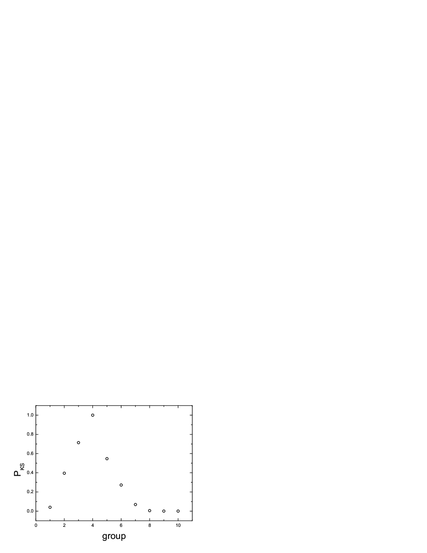
Figure 10: The plots of $P_{KS}$ and groups for the cases of shifttime (left panel) and normalizedshifttime (right panel), where the $P_{KS}$ are the significance probability between group 4 and all the groups after our sample being divided into 10 groups in terms of shifttime and normalizedshifttime.

Since many pulses have a shapes like FRED but one can not prove that all pulses have such a shape. We check the ratios of rise width to decay width of our selected sample (see Table 1). The ratios are obtained by using the best model parameters due to it can reflect the profile of corresponding pulse. As Koceviski et al. (2003) described that KRL function is an analytical function based on physical first principles and well-established empirical descriptions of GRB spectral evolution. These analytical profiles are independent of the emission mechanism and can be fully model the FRED light curve. While Norris et al. (1996) pointed out that the Norris function are more flexible model. It can model that pulses with various shapes, especially for the sharp peak pulse, and would not be constrained in the shapes of FRED. Therefore, we think that the two models can well present the pulse shapes and can get satisfied results. The histogram of ratios is displayed in Figure 3. It is found that the ratios clustered at less than unit, which is consistent with the remarks given by Norris et al. (1996) and Lee et al. (2000a, 2000b). With the ratios less than unit we deem these pulses are similar to FRED pulses. Since the pulse could be not presented by only one functional form, we consider one of possible reasons of the ratios more than unit come from the functional form, or could be cause by the pulses overlap. It is suspected that, to some extent, the evolution of $E_{peak}$ of tracking pulses is related to the time profile.

5 conclusions and discussion

In this paper, we investigate a sample including 42 tracking pulses within 36 GRBs involved 527 time-resolved spectra and study the evolutionary characteristics of $E_{peak}$. The sample consist of 29 bright and 7 weak BATSE GRBs. In order to get good statistics, we use a S/N of the observations of at least $\sim$ 30 and arrive at $\sim$ 45 as much as possible for the time-resolved spectroscopy. Since the work focus on separate tracking pulse, we adopt two pulse models to obtain better identification of the selected pulses and discard that with large fitting $\chi_{\nu}^{2}$ ($>$2). Therefore, we think that our sample is very representative of tracking pulses.

In order to make the time a relative uniform standard, we first make a transformation of the time since trigger relative to the time of maximum intensity of pulses (shifttime) and normalize the shifttime in the width of pulse (normalizedshifttime). We find that the evolution of $E_{peak}$ indeed follow soft-to-hard-to-soft with both of shifttime and normalizedshifttime (see Figure 3). Then we divide evenly our sample into 10 groups according to the two time order to study the evolution of median as well as the ratios of above 200 keV, 100 keV and 50 keV. For this type of tracking pulse the $E_{peak}$ of rise phase always larger than 50 keV, while some spectra in the decay phase less than 50 keV. The spectra of rise phase are harder than that of decay phase. In addition, we find that the rise phase of $E_{peak}$ evolution are shorter than that of the decay phase and this trends are established in our selected pulses.

As the previous section pointed out the $E_{peak}$ of time resolved spectra are fitted by COMP model. Is there a bias introduced in always using the COMP model when the Band model is the appropriate model? Therefore we also investigate the time resolved spectra of some pulses using Band and COMP model and then compare the values of $E_{peak}$ when the fitting $\chi_{\nu}^{2}$ of Band model are smaller than or comparable to that of COMP model. We find that this lead to a little high $E_{peak}$ estimates and slightly high $E_{peak}$’s during the rise phases.

The observed gamma-ray pulses are believed to be produced in a relativistically expanding and collimated fireball because of the large energies and the short time-scales involved. To account for the observed spectra of bursts, the Doppler effect over the whole fireball surface (or the curvature effect) would play an important role (e.g. Meszaros and Rees 1998; Hailey et al. 1999; Qin 2002, 2003). The Doppler model is the model describing the kinetic effect of the expanding fireball surface on the radiation observed, where the variance of the Doppler factor and the time delay caused by different emission areas on the fireball surface (or the spherical surface of uniform jets) are the key factors to be considered (for a detailed description, see Qin 2002 and Qin et al. 2004).

Qin et al. (2006) investigated the GRBs pulses and found that the curvature effect influences the evolutionary curve of the corresponding hardness ratio. They found the evolutionary curve of the pure hardness ratio would peak at the very beginning of the curve, and then would undergo a drop-to-rise-to-decay phase due to the curvature effect.

Based on the model of highly symmetric expanding fireballs, Lu et al. (2007) investigated in detail the evolution of spectral hardness $E_{peak}$ of FRED pulse caused by curvature effect. They first investigated the cases that the local pulses are exponential rise and exponential decay and exponential rise, respectively, and found that for both of the two local pulses the evolutionary curves of $E_{peak}$ underwent drop-to-rise-to-decay evolution, which corresponded to A, B, and C phases, respectively. Then they assumed that the local pulses was exponential rise and exponential decay pulse as well as the rest frame spectra varied with time, the same result were obtained. The B and C phase correspond to the rise phase (soft-to-hard) and decay phase (hard-to-soft). We can also find from Figure 1 and 3 in Lu et al. (2007) that the time interval of B phase is shorter than that of C phase and the spectra of the B phase are harder than that of the C phase. This situation are in good agreement with the conclusions of the our selected pulses. Why the A phase in our sample are not observed by BATSE? The main cause we consider that it corresponds to the very onset of the light-curve pulse, where the real emissions are always contaminated by the background.

Therefore, we think the evolution of the $E_{peak}$ in our selected pulses can be mainly caused by Doppler effect and argue that kinematics effect may be play important role in the course of spectral evolution.

In view of dynamics, the current popular views on the production of GRB is the synchrotron shock model. Based on this model, a soft-to-hard co-moving spectrum might be come into being in the case of a synchrotron radiation when electrons radiate at the beginning of a shock gaining accelerations and then arriving at the maximum speeds. The phase may be very short. After the hardest spectrum appears, the electrons start to decelerate and the energy of electrons become small. Moreover, the curvature effect must be at work because the radiation come from different latitudes of fireball (or angles of line of sight). Both of aforementioned two factors cause the observed spectra evolute from hard to soft. The phase must be much longer than that of the soft-to-hard (see Figure 8 and Table 2).

Kobayashi et al. (1997) discussed the possibility that GRBs result from internal shocks in ultrarelativistic matter and provide the pulse profile of internal shock in Figure 1. From Figure 1 given by Kobayshi et al. (1997) we can find that the radiation power of internal shock indeed follow weak-to-strong-to-weak, moreover, the time of weak-to-strong are shorter than that of the strong-to-weak. This characteristic are consistent with that of $E_{peak}$ of the tracking pulses, which indicate that this type of tracking pulses also are related to the process of internal shock. Therefore, our results for the tracking pulses do clearly support the models of GRB shocks.

Consequently, we argue that the spectral evolution of tracking pulses may be relate to both of kinematic and dynamic process. Maybe the two processes play important roles together or only one is dominant, which are unclear and deserve the further investigation. Our detailed statistical results of $E_{peak}$ evolution of tracking pulses must be constrain the current theoretic model for the fact that spectral properties of bursts can provide powerful constrains on the detailed physical models.

In this work, we only concentrate our attention on the tracking pulses and have not attempted to study non-tracking pulses or to show that all pulses must be tracking pulses. We also consider and investigate whether all pulses (or just most pulses) are hard-to-soft or tracking. For the 34 weak burst pulses provided by Kocevski et al. (2003) we find they are either hard-to-soft or tracking. In addition, the fraction of tracking pulses is about 24 percent. However, we can not afford correctly the evolutionary forms and the fraction of tracking pulses of most bright bursts because there are many short pulses and the data points of $E_{p}eak$ are few. We only give the statistical properties of tracking pulses, which will help us rule on the nature of GRB pulses as tracking.

We thank the anonymous referee for constructive suggestions and Yi-Ping Qin for his helpful discussions. Thanks are also given to Rorbet Preece and Yuki Kaneko for their help with RMFIT. This work was supported by the Natural Science Fund for Young Scholars of Yunnan Normal University (2008Z016 ), the National Natural Science Foundation of China (No. 10778726, 10747001), and the Natural Science Fund of Yunnan Province (2006A0027M).

References

- Band et al., (1992) Band, D., et al. 1992, AIPC, 265, 169
- Band et al. (1993) Band, D., et al. 1993, ApJ, 413, 281
- Band et al. (1997) Band, D., 1997, ApJ, 486, 928
- 357Bhat, (1994) Bhat, P. N., et al., 1994, ApJ, 426, 604
- Briggs (1996) Briggs, M. S. 1996, in AIP Conf. Proc. 384, Gamma-Ray Bursts, 3rd Huntsville Symp., ed. C. Kouveliotou, M. Briggs, & G. Fishman (New York: AIP), 133
- Butler et al. (1997) Butler, N. R., Kocevski, D., 2007, ApJ, 663, 407
- Crider et al. (1997) Crider, A., et al. 1997, ApJ, 479, L39
- Fishman et al. (1994) Fishman, G., et al. 1994, ApJS, 92, 229
- 141Ford, (1995) Ford, L. A., et al. 1995, ApJ, 439, 307
- 353Golenetskii, (1983) Golenetskii, S. V., et al. 1983, Nature, 306, 451
- Hailey (1999) Hailey, C. J., et al. 1999, ApJ, 520, L25
- 358Kaneko, (2006) Kaneko, Y., et al. 2006, ApJS, 166, 298 (Paper I)
- 356Kargatis, (1994) Kargatis, V. E., et al. 1994, ApJ, 422, 260
- 310Kobayashi, (1997) Kobayashi, S., et al. 1997, ApJ, 490, 92
- Kocevski et al. (2003) Kocevski, D., et al. 2003, ApJ, 596, 389
- Laros et al. (2007) Laros, J. G., et al. 1985, ApJ, 290,728
- Lee et al. (2000) Lee, A., et al. 2000a, ApJS, 131, 1
- Lee et al. (2000) Lee, A., et al. 2000b, ApJS, 131, 21
- Liang et al. (1997) Liang, E. P., et al. 1997, ApJ, 476, L35
- Lu et al. (2007) Lu, R. J., et al. 2007, ApJ, 663, 1110
- Nemiroff (2000) Mallozzi, R. S., et al. 2005, RMFIT, A Lightcurve and Spectral Analysis Tool, ( Huntsville: Univ. Alabama)
- Maszaros, (1998) Maszaros, P., Rees, M. J. 1998, ApJ, 502, L105
- 355Norris, (1986) Norris, J. P., et al., 1986, ApJ, 301, 213
- Norris et al. (1996) Norris, J. P., et al. 1996, ApJ, 459, 393
- Pendleton (1997) Pendleton, G. N., et al. 1997, ApJ, 489, 175
- Peng et al. (2000) Peng, Z. Y., et al. 2006, MNRAS, 368, 1351
- Preece et al. (1998) Preece, R. D., et al. 1998, ApJ, 496, 849
- Preece et al. (2000) Preece, R. D., et al. 2000, ApJS, 126, 19
- Press et al. (1992) Press et al. 1992, Numerical Recipes in FORTRAN (2nd ed.; New York: Cambridge Univ. Press)
- Qin (2002) Qin, Y.-P. 2002, A&A, 396, 705
- Qin (2003) Qin, Y.-P. 2003, A&A, 407, 393
- Qin (2004) Qin, Y.-P., et al. 2004, ApJ, 617, 439
- Qin et al. (2006) Qin, Y.-P., et al. 2006, Phys. Rev. D, 74, 063005
- Ryde and Svensson (2002) Ryde, F., Svensson, R. 2002, ApJ, 566, 210
- Ryde and Petrosian (2002) Ryde, F., et al. 2005, A & A, 432, 105
- 130Share, (1998) Share, G. H., Matz, S. M., 1998, AIPC, 428, 354
- 130Share, (1998) Wheaton, W. A., et al. 1973, ApJ, 185, L57