The initial value problem for linearized gravitational perturbations of the Schwarzschild naked singularity

Abstract

The coupled equations for the scalar modes of the linearized Einstein equations around Schwarzschild’s spacetime were reduced by Zerilli to a 1+1 wave equation $\partial^{2}\Psi_{z}/\partial t^{2}+{\cal H}\Psi_{z}=0$, where ${\cal H}=-\partial^{2}/\partial x^{2}+V(x)$ is the Zerilli “Hamiltonian”, $x$ the tortoise radial coordinate. From its definition, for smooth metric perturbations the field $\Psi_{z}$ is singular at $r_{s}=-6M/(\ell-1)(\ell+2)$, with $\ell$ the mode harmonic number. The equation $\Psi_{z}$ obeys is also singular, since $V$ has a second order pole at $r_{s}$. This is irrelevant to the black hole exterior stability problem, where $r>2M>0$, and $r_{s}<0$, but it introduces a non trivial problem in the naked singular case where $M<0$, then $r_{s}>0$, and the singularity appears in the relevant range of $r$ ( $0<r<\infty$). We solve this problem by developing a new approach to the evolution of the even mode, based on a new gauge invariant function, $\hat{\Psi}$, that is a regular function of the metric perturbation for any value of $M$. The relation of $\hat{\Psi}$ to $\Psi_{z}$ is provided by an intertwiner operator. The spatial pieces of the $1+1$ wave equations that $\hat{\Psi}$ and $\Psi_{z}$ obey are related as a supersymmetric pair of quantum hamiltonians ${\cal H}$ and $\hat{\cal H}$. For $M<0$, $\hat{\cal H}$ has a regular potential and a unique self-adjoint extension in a domain ${\cal D}$ defined by a physically motivated boundary condition at $r=0$. This allows to address the issue of evolution of gravitational perturbations in this non globally hyperbolic background. This formulation is used to complete the proof of the linear instability of the Schwarzschild naked singularity, by showing that a previously found unstable mode belongs to a complete basis of $\hat{\cal H}$ in ${\cal D}$, and thus is excitable by generic initial data. This is further illustrated by numerically solving the linearized equations for suitably chosen initial data.

I Introduction

The linear stability under gravitational perturbations of the negative mass Schwarzschild spacetime was first considered in ghi , where a proof of stability for the vector (or odd) modes is given. For the scalar (even) modes, reconsidered in dg , the problem is far more subtle, because the behaviour of the Zerilli potential $V_{z}$ zerilli ; ki at $x=0$ (which corresponds to the $r=0$ Schwarzschild singularity) implies a one parameter ambiguity ghi in boundary conditions at this point (parameterized by $\theta\in S^{1}$, see equation (21) below), and also because $V_{z}$ has a second order pole at $r=r_{s}:=-6M/(\ell-1)(\ell+2)$ which falls within the domain of interest for negative $M$. None of these problems are present in the positive mass case, for which the relevant range is $r>2M$ (mapped over $-\infty<x<\infty$), and $r_{s}<0$.

The ambiguity in boundary conditions at $x=0$ was addressed to in ghi ; dg , where it was shown that $\Psi_{z}\sim x^{1/2}$ as $x\to 0^{+}$ is to be selected in order that the first order corrections to the Riemann tensor algebraic invariants do not diverge faster than their zeroth order piece as the singularity is approached, a natural requirement if one wants the first order formalism to provide approximate solution of Einstein’s equations that can be consistently interpreted as arbitrarily small perturbations of the unperturbed metric. This choice also selects perturbations with finite energy, using the energy notion obtained by going to second order perturbation theory ghi ; dg . The singularity of $V_{z}$ at $r=r_{s}$ is called a “kinematic” in dg , because it is due to the fact that, as defined, the Zerilli function $\Psi_{z}$ has a simple pole at this point for generic smooth gravitational perturbations (see dg and Lemma 1, equation (18) below.) In the Zerilli formulation zerilli ; ki , the initial value problem (IVP) for linearized gravity around the $M<0$ Schwarzschild spacetime can then be posed as follows: given $\Psi_{z}(t=0,x),\dot{\Psi}_{z}(t=0,x)$ defined for $x>0$, both satisfying (18) and vanishing as $x^{1/2}$ -or faster- for $x\to 0^{+}$, find the unique $\Psi(t,x)$ obeying the singular equation equation (9)-(12) in the half space $x>0$, and giving this data for $t=0$.
The purpose of this paper is to solve this rather bizarre IVP. The exterior black hole ($r>2M>0$) Zerilli equation is entirely free of difficulties, it is a $1+1$ wave equation in a complete Minkowskian space (the horizon lying at the tortoise coordinate value $x=-\infty$), with a smooth potential, and initial data can be evolved by ${\cal H}$ mode expansion. The difficulties for the $M<0$ case cannot be overcome by introducing alternative radial variables or integrating factors, which can be easily seen to merely move the singularity from the coefficients of the differential equation to the measure that makes its radial piece self adjoint. Solving the IVP for $M<0$ allows us to complete the proof in dg that the negative mass Schwarzschild spacetime is unstable under linear gravitational perturbations, as part of a program to study the linear stability of the most notable nakedly singular solutions of Einstein’s equation dgp ; dgsv , in connection to cosmic censorship. Unstable (exponentially growing in time) modes were not only found for the negative mass Schwarzschild spacetime dg , but also for the $|Q|>M$ Reissner Nördstrom and the $|J|>M^{2}$ Kerr naked singularities dgp ; dgsv . The instability for the negative mass Schwarzschild -(A)dS and the negative mass Reissner-Nördstrom spacetimes were proved in cardo . The unstable smooth solutions of the $M<0$ Schwarzschild linearized Einstein equations in dg , satisfy the desired boundary condition at $r=0$, and decay exponentially for large $r$. It is argued in dg that they can be excited by initial data compactly supported away from $r=0$, but this can not be proved if we do not know how to evolve initial data. In this paper we show how the IVP for even perturbations on a negative mass Schwarzschild spacetime can be solved by using the technique of intertwining operators (see price and references therein). An intertwining operator ${\cal I}=\partial/\partial x+g(x)$ is constructed such that for regular metric perturbations $\hat{\Psi}:={\cal I}\Psi_{z}$ is smooth and belongs to $L^{2}((0,\infty),dx)$. $\hat{\Psi}$ satisfies a Zerilli like equation $0=[\partial^{2}/\partial t^{2}+\hat{\cal H}]\hat{\Psi}$, $\hat{\cal H}:=-\partial^{2}/\partial x^{2}+\hat{V}$, with a potential $\hat{V}$ that is free of singularities and such that $\hat{\cal H}$ has a unique self adjoint extension in a domain ${\cal D}\subset L^{2}((0,\infty),dx)$, that corresponds precisely to our physically motivated choice of boundary condition at $x=0$.

These two key differences with the standard Zerilli approach allow us to give a comprehensive answer to the linear stability problem of $M<0$ Schwarzschild spacetime, as we can show that physically sensible initial data supported away from the singularity generically excites the unstable modes found in dg . As is shown in Section III, this is not related to the $x=0$ boundary conditions; if a perturbation is initially supported away from the singularity, the unstable modes are excited before the excitation reaches the singularity.

In Section II we give a brief account of Zerilli’s approach to (even type) gravitational perturbations of Schwarzschild spacetime, stressing the problems that arise in the negative mass case. We exhibit the unstable modes found in dg , and introduce the new field $\hat{\Psi}$, which is smooth for smooth metric perturbations, no matter the sign of $M$, and obeys an equation free of singularities for any $M$. The main results of this paper are listed in a theorem, proved in Section IV, from which the negative mass Schwarzschild spacetime linear instability follows as a corollary. In Section III we illustrate, by means of numerical integrations of the linearized equations, how the unstable linear mode found in dg for the negative mass Schwarzschild spacetime is excited by perturbations with different initial data. Section V summarizes our results.

II Scalar gravitational perturbations of the Schwarzschild spacetime

In the Regge-Wheeler gauge rw , the scalar perturbations for the angular mode $(\ell,m)$ are described by four functions $H_{0}(r,t)$, $H_{1}(r,t)$, $H_{2}(r,t)$ and $K(r,t)$, in terms of which the perturbed metric takes the form,

$$ds^{2} = -\left(1-\frac{2M}{r}\right)\left(1-\epsilon H_{0}Y_{\ell,m}\right)dt^{2}+2\;\epsilon H_{1}Y_{\ell,m}dtdr+\left(1-\frac{2M}{r}\right)^{-1}\left(1+\epsilon H_{2}Y_{\ell,m}\right)dr^{2}$$ (1)

$$+r^{2}\left(1+\epsilon K\,Y_{\ell,m}\right)\left(d\theta^{2}+\sin^{2}(\theta)d\phi^{2}\right)$$

where $Y_{\ell,m}=Y_{\ell,m}(\theta,\phi)$ are standard spherical harmonics on the sphere. The linearized Einstein equations for the metric (1), obtained by disregarding terms of order $\epsilon^{2}$ or higher, imply $H_{0}(r,t)=H_{2}(r,t)$, and a set of coupled differential equations for $H_{1}$, $H_{2}$ and $K$.

Of particular interest to us is the following unstable solution found in dg for the negative mass case:

$$K(t,r) = \frac{(\lambda+1)(r-2M)^{k}}{6M}\exp\left[\frac{k(t-r)}{2|M|}\right]$$ (2)

$$H_{1}(r,t) = -H_{2}(t,r)=-\frac{\lambda(\lambda+1)[2(\lambda+1)r-6M]\;r(r-2M)^{k-1}}{36M^{2}}\exp\left[\frac{k(t-r)}{2|M|}\right]$$

where

$$k=\frac{(\ell-1)\ell(\ell+1)(\ell+2)}{6},$$ (3)

and

$$\lambda=\frac{(\ell-1)(\ell+2)}{2}.$$ (4)

The above solution has the following properties (see Section 7 in dg ): (i) it is exponentially growing in time, (ii) it is smooth for $r>0$, exponentially decaying for large $r$; (iii) it has a fast decay as $r\to 0^{+}$ that guarantees that the first order algebraic and differential invariants of the Riemann tensor do not diverge faster than their zeroth order piece, a condition of self consistence of the perturbation procedure, (iii) it has finite gravitational energy $E_{G}$

$$E_{G}=-\frac{1}{8\pi}\int_{\Sigma_{(3)}}G^{(2)}_{ab}\eta^{a}\zeta^{b}d\Sigma_{(3)},\hskip 28.45274pt\eta=(1-2M/r)^{-1/2}\partial/\partial t,\;\;\;\zeta=\partial/\partial t,$$ (5)

where $G^{(2)}_{ab}$ is the second order correction to the Einstein tensor, and $\Sigma_{(3)}$ the spacelike hypersurface orthogonal to $\eta^{a}$ (for details see ghi ; dg ; chandra .)

As shown below, the evolution of generic initial data with compact support away from the singularity will excite these singular modes, which implies that the negative mass Schwarzschild spacetime is linearly unstable. We first recall Zerilli’s approach to the linearized problem, in order to exhibit the difficulties in dealing with the evolution of initial data for the Schwarzschild spacetime in the negative mass case, and develop an alternative approach to the linearized problem that allows us to overcome these problems.

II.1 Solution of the even mode linearized Einstein equations: Zerilli’s approach

The linearized Einstein’s equation for (1) give a coupled system of partial differential equations involving $K,H_{1}$ and $H_{2}$ rw . This system can be decoupled by introducing the Zerilli function $\Psi_{z}(t,r)$, by the replacements zerilli ,

$$K = q(r)\Psi_{z}+\left(1-\frac{2M}{r}\right)\frac{\partial\Psi_{z}}{\partial r}$$

$$H_{1} = h(r)\frac{\partial\Psi_{z}}{\partial t}+r\frac{\partial^{2}\Psi_{z}}{\partial t\partial r}$$ (6)

$$H_{2} = \frac{\partial}{\partial r}\left[\left(1-\frac{2M}{r}\right)\left(h(r)\Psi_{z}+r\frac{\partial\Psi}{\partial r}\right)\right]-K$$

where $\lambda$ is defined in (4) and

$$q(r) = \frac{\lambda(\lambda+1)r^{2}+3\lambda Mr+6M^{2}}{r^{2}(\lambda r+3M)},$$ (7)

$$h(r) = \frac{\lambda r^{2}-3\lambda rM-3M^{2}}{(r-2M)(\lambda r+3M)}.$$

Note that the relations (II.1) can be inverted and give

$$\Psi_{z}(r,t)=\frac{r(r-2M)}{(\lambda+1)(\lambda\,r+3\,M)}\left(H_{2}-r\frac{\partial K}{\partial r}\right)+\frac{r}{\lambda+1}K.$$ (8)

The full set of linearized Einstein’s equations then reduce to Zerilli’s wave equation

$$\frac{\partial^{2}\Psi_{z}}{\partial t^{2}}+{\cal H}\Psi_{z}=0,$$ (9)

where,

$${\cal H}=-\frac{\partial^{2}}{\partial x^{2}}+V$$ (10)

looks like a quantum Hamiltonian operator with potential

$$V=2\left(1-\frac{2M}{r}\right){\frac{\lambda^{2}r^{2}\left[(\lambda+1)r+3M\right]+9M^{2}(\lambda r+M)}{r^{3}(\lambda r+3M)^{2}}},$$ (11)

and $x$ is the “tortoise” coordinate, related to $r$ by

$$\frac{dx}{dr}=\left(1-\frac{2M}{r}\right)^{-1}.$$ (12)

We will choose the integration constant such that $x=0$ at $r=0$, then

$$x=r+2M\ln\left|\frac{r-2M}{2M}\right|.$$ (13)

II.1.1 Case $M>0$, stability of the Schwarzschild black hole exterior metric

For $M>0$, the exterior static region $r>2M$ of the Schwarzschild black hole gets mapped under (13) onto $-\infty<x<\infty$, with the black hole horizon sitting at $x=-\infty$. The potential $V$ in Zerilli’s equation is positive definite and behaves as $V\sim\exp(x/(2M))$ as $x\to-\infty$, $V\sim x^{-2}$ as $x\to\infty$ (see Figure 1). Equation (8) indicates that a smooth metric perturbation with compact support in the exterior region corresponds to a smooth Zerilli function in $L^{2}({\mathbb{R}},dx)$. The fact that $\Psi_{z}^{0}:=\Psi_{z}\mid_{(t=0,x)}$ and $\dot{\Psi}_{z}^{0}:=\partial/\partial t\Psi_{z}\mid_{(t=0,x)}$ can be freely chosen, together with (II.1), takes proper account of the constraints among the initial data for $H_{1},H_{2}$ and $K$. To solve the Zerilli wave equation (9) from a given initial data $(\Psi_{z}^{0},\dot{\Psi}_{z}^{0})\in L^{2}({\mathbb{R}},dx)\otimes L^{2}({\mathbb{R}},dx)$, we can use that ${\cal H}$ is a self adjoint operator in $L^{2}({\mathbb{R}},dx)$ to expand $\Psi_{z}^{0}$ and $\dot{\Psi}_{z}^{0}$ using a complete set $\psi_{E}$ of eigenfunctions of ${\cal H}$ (${\cal H}\;\psi_{E}=E\psi_{E}$). Equation (9) then reduces to the following ordinary differential equations for $a_{E}(t):=\int\psi_{E}(x)^{*}\Psi_{z}(t,x)dx$:

$$\ddot{a}_{E} = -Ea_{E}$$

$$\dot{a}_{E}(0) = \dot{a}_{E}^{0}:=\int\psi_{E}^{*}\dot{\Psi}_{z}^{0}\;dx$$ (14)

$$a_{E}(0) = a_{E}^{0}:=\int\psi_{E}^{*}\Psi_{z}^{0}\;dx.$$

whose solution is

$$a_{E}(t)=\begin{cases}a_{E}^{0}\;\cos(\sqrt{E}t)+\dot{a}_{E}^{0}\;E^{-1/2}\;\sin(\sqrt{E}t)\ &,E>0\\ a_{E}^{0}+t\;\dot{a}_{E}^{0}&,E=0\\ a_{E}^{0}\;\cosh(\sqrt{-E}t)+\dot{a}_{E}^{0}\;(-E)^{-1/2}\;\sinh(\sqrt{-E}t)&,E<0\end{cases}$$ (15)

Since the Zerilli Hamiltonian ${\cal H}$ is positive definite, we can use the above equations to obtain and $L^{2}$ bound for $\Psi$ at time $t$ in terms of its data wald as

$$\int|\Psi|^{2}dx\leq 2\left(\int|\Psi^{0}|^{2}dx+\int\overline{\dot{\Psi}^{0}}\;{\cal H}^{-1}\dot{\Psi}^{0}dx\right),$$ (16)

where the inverse of ${\cal H}$ is defined using its spectral decomposition. The detailed analysis in wald gives also the following uniform bound for the Zerilli function in terms of the initial data

$$|\Psi_{z}(t,x)|^{2}\leq\int\left(|\Psi_{z}^{0}|^{2}+\frac{1}{2}\overline{\Psi_{z}^{0}}\;{\cal H}\;\Psi_{z}^{0}+\frac{1}{2}|\dot{\Psi}_{z}^{0}|^{2}+\overline{\dot{\Psi}^{0}}\;{\cal H}^{-1}\dot{\Psi}^{0}\right)dx$$ (17)

This proves that the exterior, static region of a Schwarzschild black hole is stable.

         

Figure 1: The left panel shows the $\ell=2$ Zerilli potential for $M=3$ as a function of $x$. The black hole horizon is located at $x=-\infty$. Note that the potential is smooth and positive. The right panel shows the $\ell=2$ Zerilli potential for $M=-2$. The naked singularity is located at $x=0$. The “kinematic” double pole is at $x\simeq 0.761$.

II.1.2 Case $M<0$, stability of the Schwarzschild naked singularity

For $M<0$ the range of interest is $r>0$ (then $x>0$), and a number of difficulties arise due to the fact that $q$ and $h$ in (7) are singular at $r=r_{s}:=-3M/\lambda>0$, and that this point belongs to the domain of interest. This implies that $\Psi_{z}$ is singular at $r_{s}$, as is also evident from equation (8). The kind of singularity in $\Psi_{z}$ is characterized in the following lemma:

Lemma 1: If $M<0$, a metric perturbation is smooth if and only if its Zerilli function at any fixed time is $C^{\infty}$ in open sets not containing $r_{s}$, and admits a Laurent expansion

$$\Psi_{z}=\sum_{j\geq-1}c_{j}(r-r_{s})^{j},\;\;\;c_{0}=\frac{\lambda^{2}c_{-1}}{3M(3+2\lambda)}$$ (18)

If initial data $\Psi_{z}^{0}$ and $\dot{\Psi}_{z}^{0}$ is given, both functions satisfying (18), the evolution equation will preserve (18), i.e., this condition will hold at all times.

Proof: From (II.1) and (7), the metric perturbation will be smooth if and only if $h(r)\Psi_{z}+r\frac{\partial\Psi_{z}}{\partial r}$ and $q(r)\Psi_{z}+(1-2M/r)\frac{\partial\Psi_{z}}{\partial r}$ are smooth. Both conditions lead to (18), added to smoothness in open sets not containing $r_{s}$. A straightforward calculation shows that if $\psi$ satisfies (18) then so does ${\cal H}\psi$. This guarantees that this condition will hold at later times if it is satisfied by the initial data $\Box$

In particular, Zerilli functions for smooth metric perturbations are generically not square integrable (no matter which measure we use, either $dx=dr/(1-2M/r)$ or $dr$) due to the pole in (18). As an example, the smooth $M<0$ metric perturbation (2) has the singular Zerilli function

$$\Psi_{z}^{unst}=\frac{r\left(r-2M\right)^{k}}{2\lambda r+6M}\exp\left[\frac{k(t-r)}{2|M|}\right]=:\exp\left[\frac{kt}{2|M|}\right]\psi^{unst}.$$ (19)

Given that $\Psi_{z}$ is a singular function of the metric perturbation, it is not a surprise that the coefficients of the differential equation it obeys are singular. This explains the second order pole of the Zerilli potential at $r_{s}$ (and the name “kinematic” given in dg to this singularity.) Note that the approach for solving Zerilli’s equation in the $M>0$ case completely breaks down when $M<0$ since (i) $\Psi_{z}\not\in L^{2}((0,\infty),dx)$ and (ii) $V$ has the kinematic singularity. In particular, the associated quantum mechanical problem with Hamiltonian ${\cal H}$ and domain $x\in(0,\infty)$ is not relevant in this case because of (i), as discussed in detail in Section 7 of dg . Furthermore, since (9) is a wave equation in the half space $x>0$, we need to specify boundary conditions at $x=0$, besides the initial values of $\Psi_{z}^{0}$ and $\dot{\Psi}_{z}^{0}$, to have a unique solution. The fact that the potential has a singularity at the boundary,

$$V\simeq-1/(4x^{2})+...\;\;\text{ for }\;x\to 0^{+}.$$ (20)

implies that there is an infinite number of (formally, i.e., ignoring the kinematic singularity) self-adjoint extensions of ${\cal H}:=-\partial^{2}/\partial x^{2}+V$, parameterized by $\theta\in S^{1}$, obtained by demanding that the Zerilli function behaves as

$$\Psi_{z}\simeq\cos(\theta)\left[\left(\frac{x}{|M|}\right)^{1/2}+...\right]+\sin(\theta)\left[\left(\frac{x}{|M|}\right)^{1/2}\ln\left(\frac{x}{|M|}\right)+...\right]$$ (21)

for $x\gtrsim 0$ (the terms in square brackets are the leading terms of two linearly independent local solutions of the eigenvalue equation ${\cal H}\Psi=E\Psi$, $E$ shows up at higher orders). Note that both linearly independent local solutions in (21) are square integrable near $x=0$, the potential belongs to the “limit circle class” at $x=0$ reed . This issue was analyzed in detail in ghi (see also meetz and reed ) where it was concluded that $\theta=0$ is a physically motivated choice, since it corresponds to finite energy perturbations with first order contributions to the Kretschmann invariant not diverging faster than its zeroth order piece. These results were confirmed in dg , where it was further shown that every algebraic and some of the differential invariants made out of the Riemann tensor share this property with the Kretschmann invariant. Given that this guarantees the self consistency of the linearized treatment, we will be restrict our attention to the case $\Psi_{z}\sim x^{1/2}$ from now on.

The question left open in dg is how to evolve initial perturbation data in the $M<0$ case, since the ${\cal H}$ mode expansion technique used for $M>0$ does not apply to the $M<0$ case. In the next Section we introduce a field $\hat{\Psi}$ which is smooth for smooth metric perturbation, and evolves according to a wave equation with a smooth potential for any sign of $M$, thus providing a solution to the initial value problem in the negative mass case.

II.2 Solution of the even mode linearized Einstein equations: alternative approach

As explained above, the quantum mechanical problem associated to ${\cal H}$ is not directly relevant to the gravitational perturbation problem when $M<0$. Zerilli’s function succeeds in reducing the full set of linearized Einstein’s equations to a single wave equation, however, for $M<0$, this function is singular in the relevant $r>0$ range. The “kinematic” singularity at $r_{s}=-3M/\lambda$ in (8) indicates that physically acceptable Zerilli functions have a simple pole at $r_{s}$ (Lemma 1). Thus, even if ${\cal H}$ could be extended to a self adjoint operator in some subspace of $L^{2}({\mathbb{R}},dx)$, this space would not be the natural setting for physically acceptable gravitational perturbations, which, because of the kinematic singularity, correspond, generically, to functions that are not square integrable.

In terms of the Zerilli function, the evolution problem in the negative mass case is: given data $\Psi_{z}^{0},\dot{\Psi}_{z}^{0}$ both satisfying the conditions in Lemma 1, and vanishing as $x^{1/2}$ when $x\to 0^{+}$ (i.e., (21) with $\theta=0$), find $\Psi_{z}$ for later times. The approach of solving this problem by separation of variables in Zerilli’s wave equation and expanding by ${\cal H}$ modes fails. A satisfactory solution to the evolution problem requires finding a new field $\hat{\Psi}$ that decouples the linearized equations obeyed by $K,H_{1}$ and $H_{2}$ -as $\Psi_{z}$ does-, and that is a smooth function of $K,H_{1}$ and $H_{2}$ for any value of $M$. In this section we show how this is done. We will state without proof our main result (Theorem below), and illustrate for the $\ell=2$ mode, case in which the explicit formulae are relatively simple. We will defer the proof of the theorem to section IV

Theorem: Let $\psi_{0}$ be the solution of ${\cal H}\psi_{0}=0$ given in equations (52) and (55). Define $g:=\psi_{0}{}^{\prime}/\psi_{0}$ (a prime denotes derivative with respect to $x$) and the operators

$${\cal I} := \frac{\partial}{\partial x}-g,$$ (22)

$$\hat{\cal I} := \frac{\partial}{\partial x}+g.$$ (23)

Let $V$ be the potential in Zerilli’s equation. Then:

1. $${\cal I}\;\left[\frac{\partial^{2}}{\partial t^{2}}-\frac{\partial^{2}}{\partial x^{2}}+V\right]=\left[\frac{\partial^{2}}{\partial t^{2}}-\frac{\partial^{2}}{\partial x^{2}}+\hat{V}\right]\;{\cal I}$$

   with $\hat{V}=V-2g^{\prime}$ smooth in the relevant domain ($r>2M$ if $M>0$, $r>0$ if $M<0$).

2. For any value of $M$, a metric perturbation (1) with Zerilli function $\Psi_{z}$ is smooth if and only if $\hat{\Psi}:={\cal I}\Psi_{z}$ is smooth in the relevant domain.

3. For $M<0$, $\hat{V}\simeq 3/(4x^{2})$ as $x\to 0^{+}$. As a consequence $\hat{\cal H}:=\frac{\partial^{2}}{\partial x^{2}}+\hat{V}(x)$ has a unique self adjoint extension in a domain ${\cal D}\subset L^{2}((0,\infty),dx)$, defined by the boundary condition $\hat{\Psi}\simeq x^{3/2}$ as $x\to 0^{+}$ (see meetz ,reed ). Moreover, for $\Psi_{z}$ as in (21), ${\cal I}\Psi_{z}\in{\cal D}$ if and only if $\theta=0$. Thus ${\cal D}$ is the set of physically relevant perturbation functions $\hat{\Psi}$.

4. Assume that $M<0$ and that $(\Psi_{z}^{0},\dot{\Psi}_{z}^{0})$ is an appropriate initial data set, i.e., it satisfies the conditions in Lemma 1 and the boundary condition $\theta=0$ in (21). Note from (iii) that both ${\cal I}\Psi_{z}^{0}$ and ${\cal I}\dot{\Psi}_{z}^{0}$ belong to ${\cal D}$. Let $\hat{\Psi}$ be the unique solution in ${\cal D}$ for the wave equation $\left[\frac{\partial^{2}}{\partial t^{2}}+\hat{\cal H}\right]\hat{\Psi}=0$ on the half space $x>0$, subject to the initial conditions $\hat{\Psi}\mid_{(t=0,x)}={\cal I}\Psi_{z}^{0}$ and $\partial/\partial t\hat{\Psi}\mid_{(t=0,x)}={\cal I}\dot{\Psi}_{z}^{0}$. This solution can be obtained by $\hat{\cal H}$ mode expansion as is done in equations (14) and (15). The Zerilli field at all times is then given by

   $$\Psi_{z}(t,x)=\int_{0}^{t}\left(\int_{0}^{t^{\prime}}\hat{\cal I}\hat{\Psi}(t^{\prime\prime},x)dt^{\prime\prime}\right)dt^{\prime}+t\dot{\Psi}_{z}^{0}+\Psi_{z}^{0}.$$ (24)

Let us clarify some aspects related to the above theorem. Generically, $\Psi_{z}$ has a pole at $r_{s}$ (Lemma 1), and so does $g$, then the operators ${\cal I}$ and $\hat{\cal I}$ are singular. The singularities cancel in such a way that $\hat{\Psi}:={\cal I}\Psi_{z}$ is smooth in the domain of interest, that is, ${\cal I}$ removes the singularity in $\Psi_{z}$. In the same way $-2g$ subtracts the pole in $V$ to produce a smooth $\hat{V}$. As an example, for $\ell=2$ we have ghi

$$\psi_{0}=\frac{r(r^{3}+3Mr^{2}-6M^{3})}{8M^{4}(3M+2r)}$$ (25)

and thus

$$\hat{V}=\frac{6(r-2M)(2r^{7}+5Mr^{6}-9M^{2}r^{5}-33M^{3}r^{4}-24M^{4}r^{3}+36M^{5}r^{2}+36M^{6}r-36M^{7})}{r^{4}(r^{3}+3Mr^{2}-6M^{3})^{2}},$$ (26)

whose only singular point lies at $r\simeq 1.2M$, which is outside the domain of interest both for positive or negative $M$. The $\ell=2$ unstable mode (19) for $M<0$ becomes

$$\hat{\Psi}^{unst}=e^{2(t-r)/|M|}\frac{r^{3}\left(r-2M\right)^{4}}{4r^{3}+12Mr^{2}+24M^{3}}=:e^{2t/|M|}\hat{\psi}^{unst},$$ (27)

which is also $C^{\infty}$ in the domain of interest. In Figure 2 we exhibit $\hat{V}$ for $\ell=2$ and $M=3$ (left), and $\hat{V}$ for $\ell=2$ and $M=-2$, superposed with the unstable mode $\hat{\psi}^{unst}$ (right).
Since the Einstein’s linearized equations reduce to the single equation

$$\left[\frac{\partial^{2}}{\partial t^{2}}+\hat{\cal H}\right]\hat{\Psi}=0,\;\;\;\hat{\Psi}\in{\cal D}$$ (28)

and $\hat{\cal H}$ is self adjoint in ${\cal D}$, we can then solve this equation by $\hat{\cal H}-$mode expansion, in the same way as is done with $\Psi_{z}$ when $M>0$. This gives an answer to the issue of evolution in the non globally hyperbolic spacetime in a way entirely analogous to that developed in wi , the only difference being that the radial part of the equations dealt with in wi are positive, essentially self adjoint operators. Note that we can work entirely in “$\hat{\Psi}$-space” with no reference to the Zerilli function (as will be done in the next section), and that our alternative formulation also works in the positive mass case. The usefulness of equation (24) lies in the simpler connection that there is between the Zerilli field and the perturbed metric elements $H_{1},H_{2}$ and $K$, equations (II.1). If we want to construct the perturbed metric elements from $\hat{\Psi}$, the shortest way seems to be inserting (24) in (II.1). Note that (24) is not an evolution equation. It just tells us how to recover the information lost after applying $\hat{\cal I}{\cal I}$ to the Zerilli function (see Section IV). In fact, we need to solve first the evolution problem for $\hat{\Psi}(t,x)$, and then use the solution $\hat{\Psi}(t,x)$ in the integrand in (24) to obtain the corresponding solution for $\Psi_{z}(t,x)$.

Corollary: The negative mass Schwarzschild solution is unstable.

Proof: The spectrum of the operator $\hat{\cal H}$ in ${\cal D}$ contains the negative eigenvalue $-k^{2}$ ($k$ given in (3)), with eigenvector $\hat{\psi}^{unst}=C\;{\cal I}\psi^{unst}$, where $\psi^{unst}$ is given in (19) and $C$ is a normalization constant. Let $a_{-k^{2}}^{0}$ and $\dot{a}_{-k^{2}}^{0}$ be the projections of $\hat{\Psi}_{0}$ and $\dot{\hat{\Psi}}_{0}$ onto this mode, (see equation (14)), then from (14) and (15) applied to (28) we obtain

$$\hat{\Psi}(t,x)=\left[a_{-k^{2}}^{0}\;\cosh(kt)+\frac{\dot{a}_{-k^{2}}^{0}}{k}\;\sinh(kt)\right]\hat{\psi}^{unst}(x)+\Phi(t,x),$$ (29)

where $\Phi(t,x)$ is a linear combination of modes $\psi_{E}$, with $E\neq-k^{2}$. Since the above decomposition is orthogonal

$$\int_{0}^{\infty}|\hat{\Psi}|^{2}dx>\left[a_{-k^{2}}^{0}\;\cosh(kt)+\frac{\dot{a}_{-k^{2}}^{0}}{k}\;\sinh(kt)\right]^{2}$$

and thus exponentially growing for large $t$ $\Box$.

Numerical evidence indicates that $\hat{\psi}^{unst}$ is the only negative eigenvalue of $\hat{\cal H}$. If this is the case, then $\Phi$ is bounded and uniformly bounded in a similar way as the positive mass Zerilli function is, equations (16) and (17).

         

Figure 2: The left panel shows the potential $\hat{V}$, for $\ell=2$ and positive mass $M=3$, as a function of $x$. The black hole horizon is located at $x=-\infty$. The right panel shows $\hat{V}$ for $\ell=2$ and $M=-2$ (solid line), and the unstable mode $\hat{\psi}_{unst}$ given (27)(dotted line). This mode satisfies $\hat{\cal H}\hat{\psi}_{unst}=-\hat{\psi}_{unst}$.

III Numerical integration of the evolution equations

Numerical integrations of the wave equation

$$\left[\frac{\partial^{2}}{\partial t^{2}}-\frac{\partial^{2}}{\partial x^{2}}-\hat{V}\right]\hat{\Psi}=0$$ (30)

subject to the boundary condition $\hat{\Psi}\simeq x^{3/2}$ as $x\to 0^{+}$ were carried out for $\ell=2$, $M=-1$ using the Maple built in integrator for partial differential equations, working in the standard radial coordinate. The boundary condition at $r=0$ was enforced by imposing Robin type boundary conditions in the form $3\hat{\Psi}-\partial\hat{\Psi}/\partial r=0$ at $r=10^{-4}$. We also set $\hat{\Psi}=0$ at $r=10$ and restricted the initial data and evolution time so that this condition is trivially satisfied. In all cases we set $\dot{\hat{\Psi}}^{0}=0$ for simplicity. We evolved different $\hat{\Psi}^{0}$ initial data sets to see how the unstable (19) mode gets excited, and the resulting numerical solution $\hat{\Psi}$ was contrasted with its expected projection $a_{-k^{2}}^{0}\;\cosh(kt)\;\hat{\psi}^{unst}(x)$ onto the unstable mode.

In the case of Figure 3, $\hat{\Psi}^{0}=\exp(-10(r-2)^{2})\Theta(r-0.0002)$, $\Theta$ a step function. If normalized, this function gives a projection $a_{-k^{2}}^{0}\simeq 0.79$ onto the unstable mode.

         

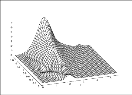
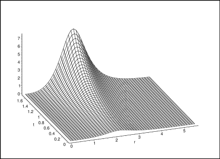
Figure 3: Left: evolution of initial data centered at $r=2$, with a strong projection onto the unstable mode. Right: time evolved unstable mode component for this data.

The unstable mode dominates for $t\gtrsim 1.6$, and it is noticeable from $t=0$. The evolution of two stable wave packets moving oppositely is also evident in the plot.

The left panel in Figure 4 shows the evolution up to $t=2.7$ of the data $\hat{\Psi}^{0}=\exp(-10(r-4)^{2})\Theta(r-0.0002),\dot{\hat{\Psi}}^{0}=0$, which has a milder projection onto the unstable mode ($a_{-k^{2}}^{0}\simeq 0.07$ when normalized). The right panel contrasts $\hat{\Psi}(t=0,r),\hat{\Psi}(t=3,r)$ and the unstable mode properly scaled by the $\cosh(6)$ factor. Note that the unstable mode is noticeable starting at $t\simeq 1.5.$

         

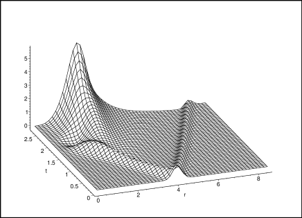
Figure 4: Left: evolution of initial data centered at $r=4$. Right: $\hat{\Psi}$ at $t=0$ (thick solid line), and $t=3$ (thin solid line), contrasted to the evolution of the unstable component at $t=3$ (dashed line).

To have a smaller overlap with the unstable mode we use $\hat{\Psi}(t=0,r)=-\exp(-10(r-4)^{2})\;\Theta(r-0.0002)\;\sin(10(r-4))$ (Figure 5, left panel). The graph may mistakenly (see equation (29)) suggest that the unstable mode is not excited before the ingoing wave packet reaches the singularity. The right panel in this figure exhibits the evolution of the projection of the initial data onto the unstable mode. This mode is initially highly suppressed because $a_{-k^{2}}^{0}\simeq 6\times 10^{-3}$

         

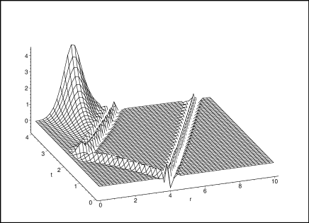
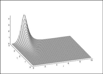
Figure 5: Left: evolution of initial data centered at $r=4$ and modulated with a sine function. The initial data has a weak projection onto the unstable mode. Right: time evolved unstable mode component for this data.

Finally, the left panel in Figure 6 exhibits the evolution of data which is almost orthogonal ($a_{-k^{2}}^{0}\simeq-2\times 10^{-10},\dot{a}_{-k^{2}}^{0}=0$) to the unstable mode. The excitation of the unstable mode reaches an amplitude $\sim 2\times 10^{-8}$ and so is unnoticeable in the displayed time range. The right panel of the figure shows the initial data (dotted line), the result of the evolution at $t=1$ (thin solid line) and the evolved data at $t=3$ (thick solid line).

         

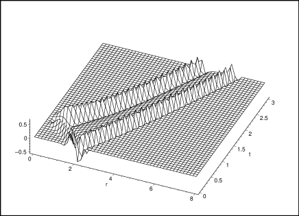
Figure 6: Left: evolution of initial data centered at $r=2$, modulated with a sine function and having a negligible projection onto the unstable mode. Right: $\hat{\Psi}$ at $t=0$ (dotted line), $t=1$ (thin solid line) and $t=3$ (thick solid line).

IV Proof of the Theorem

The alternative $\hat{\Psi}$ to the Zerilli field as a means of describing the even modes of linear gravitational perturbations is suggested by the “intertwining” potential technique in quantum mechanics price , whose original motivation is that of replacing a one dimensional quantum mechanical Hamiltonian with another Hamiltonian having a more elementary potential. We have actually used an intertwiner to replace a potential with a singularity at $r_{s}$ with one free of such singularity, with the added benefit that the resulting Hamiltonian has a unique self adjoint extension that happens to agree with the boundary condition at $r=0$ that is natural to the problem! Intertwiners appear also the context of supersymmetric quantum mechanics cooper , pairs of supersymmetric Hamiltonians being related by an intertwiner constructed using a zero energy wave function.

IV.1 Intertwining operators

Consider a two dimensional wave equation with a space dependent potential $V$

$$\left[\frac{\partial^{2}}{\partial t^{2}}-\frac{\partial^{2}}{\partial x^{2}}+V(x)\right]\Psi=0,$$ (31)

and a linear operator ${\cal I}=\frac{\partial}{\partial x}-g(x)$ such that price

$${\cal I}\;\left[-\frac{\partial^{2}}{\partial x^{2}}+V(x)\right]=\left[-\frac{\partial^{2}}{\partial x^{2}}+\hat{V}(x)\right]\;{\cal I}$$ (32)

for some potential $\hat{V}(x)$. Since ${\cal I}$ commutes with $\partial/\partial t$, any solution $\Psi$ of (31) gives a -possibly trivial- solution $\hat{\Psi}:={\cal I}\Psi$ for the equation

$$\left[\frac{\partial^{2}}{\partial t^{2}}-\frac{\partial^{2}}{\partial x^{2}}+\hat{V}(x)\right]\hat{\Psi}=0.$$ (33)

Separation of variables $\Psi=\exp(i\omega t)\psi(x)$ ( $\hat{\Psi}=\exp(i\omega t)\hat{\psi}(x)$) reduces (31) and (33) to Schrödinger like equations

$${\cal H}\psi = \left[-\frac{\partial^{2}}{\partial x^{2}}+V(x)\right]\psi=\omega^{2}\psi,$$ (34)

$$\hat{\cal H}\hat{\psi} = \left[-\frac{\partial^{2}}{\partial x^{2}}+\hat{V}(x)\right]\hat{\psi}=\omega^{2}\hat{\psi},$$ (35)

If we do not specify boundary conditions, there will be two linearly independent solutions of (34) for any chosen complex $\omega$. Let us denote any two such solutions as $\psi_{\omega}^{(j)},j=1,2$. Note from (32) that ${\cal I}\psi_{\omega}^{(j)}$ are (possibly trivial) solutions of (35).
The conditions for the existence of an intertwining operator can be obtained by applying (32) to an arbitrary function $\psi$, and then isolating terms in $\psi$ and $\psi^{\prime}:=\partial\psi/\partial x$ (the higher derivative terms cancel out). The coefficient of $\psi^{\prime}$ gives

$$\hat{V}=V-2g^{\prime}.$$ (36)

Adding the condition from the $\psi$ coefficient gives $(g^{\prime}+g^{2}-V)^{\prime}=0$, i.e. $g^{\prime}+g^{2}=V-\omega_{o}{}^{2}$ for some constant $\omega_{o}$. This last condition is more transparent if written in terms of $\psi_{\omega_{o}}:=\exp(\int^{x}g(x^{\prime})dx^{\prime})$, which satisfies $\psi_{\omega_{o}}^{\prime}/\psi_{\omega_{o}}=g$ and

$$\left[-\frac{\partial^{2}}{\partial x^{2}}+V\right]\psi_{\omega_{o}}=\omega_{o}^{2}\psi_{\omega_{o}}.$$ (37)

From this follows price ,

Lemma 2: From any solution of (37) it is possible to construct an intertwining operator ${\cal I}=\frac{\partial}{\partial x}-g(x)$ by choosing $g=\psi_{\omega_{o}}^{\prime}/\psi_{\omega_{o}}$. This gives $\hat{V}=V-2g^{\prime}$ in (32).

Lemma 2 collects the results we need from price , but we need to elaborate further on these results to get some information about the possible ways to invert the effect of ${\cal I}$. To fix the notation, let $\psi_{\omega_{o}}^{(j=1)}=\psi_{\omega_{o}}$, and $\psi_{\omega_{o}}^{(j=2)}$ be a linearly independent solutions of (37). The kernel of ${\cal I}$ is the span of $\psi_{\omega_{o}}^{(j=1)}{}$, since $0={\cal I}\psi=\psi^{\prime}-\psi_{\omega_{o}}^{(j=1)}{}^{\prime}/\psi_{\omega_{o}}^{(j=1)}{}\psi$ implies that $\psi$ is proportional to $\psi_{\omega_{o}}^{(j=1)}{}$. The form of an intertwiner $\hat{\cal I}=\frac{\partial}{\partial x}-h(x)$ satisfying

$$\hat{\cal I}\;\left[-\frac{\partial^{2}}{\partial x^{2}}+\hat{V}(x)\right]=\left[-\frac{\partial^{2}}{\partial x^{2}}+V(x)\right]\;\hat{\cal I}$$ (38)

can be guessed from Lemma 2 by noting that, since $\hat{V}-2h^{\prime}=V=\hat{V}+2g^{\prime}$, the only possible way back to $V$ is that ${\cal H}(1/\psi_{\omega_{o}}^{(j=1)}{})\propto(1/\psi_{\omega_{o}}^{(j=1)}{})$. That this is actually the case can be checked by a direct calculation using our previous results, from where we obtain $\hat{\cal H}(1/\psi_{\omega_{o}}^{(j=1)}{})=\omega_{o}{}^{2}/\psi_{\omega_{o}}^{(j=1)}{}$. We will set $\hat{\psi}{}_{\omega_{o}}^{(j=2)}:=1/\psi_{\omega_{o}}^{(j=1)}{}$ and choose $\hat{\psi}{}_{\omega_{o}}^{(j=1)}$ such that $\hat{I}\hat{\psi}{}_{\omega_{o}}^{(j=1)}=\psi_{\omega_{o}}^{(j=1)}{}$. It follows that $\hat{\cal I}:=\frac{\partial}{\partial x}+g(x)$ satisfies (38), and a simple calculation shows that $\hat{\cal I}{\cal I}\psi=(\omega_{o}{}^{2}-{\cal H})\psi$, i.e., the non trivial kernels of ${\cal I}$ and $\hat{\cal I}$ combine in such a way that the kernel of $\hat{\cal I}{\cal I}$ is the two dimensional $\omega_{o}^{2}$ eigenspace of ${\cal H}$. Note that we have shown that we can label the solutions of (37) and its hat version as such that

$$\psi_{\omega_{o}}^{(j=1)}{} = \hat{I}\hat{\psi}_{\omega_{o}}^{(j=1)}$$

$$I\psi_{\omega_{o}}^{(j=2)} = \hat{\psi}_{\omega_{o}}^{(j=2)}=1/\psi_{\omega_{o}}^{(j=1)}{}$$ (39)

$$I\psi_{\omega_{o}}^{(j=1)} = \hat{I}\hat{\psi}_{\omega_{o}}^{(j=2)}=0$$

We have proved the following

Lemma 3: The kernel of ${\cal I}=\frac{\partial}{\partial x}-\psi_{\omega_{o}}^{(j=1)}{}^{\prime}/\psi_{\omega_{o}}^{(j=1)}$ is the subspace spanned by $\psi_{\omega_{o}}^{(j=1)}$. If $\hat{\cal I}=\partial/\partial x+\psi_{\omega_{o}}^{(j=1)}{}^{\prime}/\psi_{\omega_{o}}^{(j=1)}$, then (38) holds, also

$$\hat{\cal I}{\cal I}=(\omega_{o}^{2}-{\cal H}),$$ (40)

and the solutions of ${\cal H}\psi_{\omega}=\omega^{2}\psi_{\omega}$ and $\hat{\cal H}\hat{\psi}_{\omega}=\omega^{2}\hat{\psi}_{\omega}$ can be labeled such that the equations (39) hold.

In the supersymmetric quantum mechanics context, $\omega_{o}=0$ and $\psi_{\omega_{o}}^{(j=1)}$ satisfies appropriate boundary conditions to make it an eigenfunction of ${\cal H}$. Moreover, it corresponds to the lowest eigenvalue of ${\cal H}$. In this case ${\cal H}$ and $\hat{\cal H}$ are isospectral, except for $\omega_{o}{}^{2}=0$, which is missing in the spectrum of $\hat{\cal H}$. Equations (39) then leads to the situation depicted in Fig 2.1 in cooper . In the above construction, however, we do not require any specific boundary condition on the function $\psi_{\omega_{o}}^{(j=1)}{}$ used to construct the intertwining operator.

The intertwining operator (32) will be useful whenever $\hat{V}$ is simpler than $V$. However, information is lost when solving (33) instead of (31), and we need to know how to recover it. This problem is addressed in the Lemma below.

Lemma 4: Assume $\Psi(t,x)$ satisfies the wave equation (31) with initial conditions $\Psi(0,x)=:\Psi^{0}(x)$ and $\partial\Psi/\partial t(0,x)=:\dot{\Psi}^{0}(x)$. Let $\hat{\Psi}:={\cal I}\Psi$, $\hat{\Psi}^{0}:={\cal I}\Psi^{0}$ and $\dot{\hat{\Psi}}^{0}:={\cal I}\dot{\Psi}^{0}(x)$, then:

1. $\hat{\Psi}$ satisfies the wave equation (33) with initial conditions $\hat{\Psi}(0,x)=\hat{\Psi}^{0}$ and $\partial\hat{\Psi}/\partial t(0,x)=\dot{\hat{\Psi}}^{0}$.

2. If $\omega_{o}\neq 0$, $\Psi(t,x)$ can be obtained from $\hat{\Psi}(t,x)$ by means of

   $$\Psi(t,x)=\cos(\omega_{o}t)\hat{\Psi}^{0}+\frac{\sin(\omega_{o}t)}{\omega_{o}}\dot{\hat{\Psi}}^{0}+\frac{1}{w_{o}}\left(\sin(\omega_{o}t)\int_{0}^{t}\cos(\omega_{o}t^{\prime})\hat{\cal I}\hat{\Psi}(t^{\prime},x)dt^{\prime}-\cos(\omega_{o}t)\int_{0}^{t}\sin(\omega_{o}t^{\prime})\hat{\cal I}\hat{\Psi}(t^{\prime},x)dt^{\prime}\right)$$ (41)

   For $\omega_{o}=0$ we have

   $$\Psi(t,x)=\int_{0}^{t}\left(\int_{0}^{t^{\prime}}\hat{\cal I}\hat{\Psi}(t^{\prime\prime},x)dt^{\prime\prime}\right)dt^{\prime}+t\dot{\hat{\Psi}}^{0}+\hat{\Psi}^{0}$$ (42)

Proof: (i) is trivial. To prove (ii) note from Lemma 3, equation (40), that

$$\hat{\cal I}\hat{\Psi}=\hat{\cal I}{\cal I}\Psi=(\omega_{o}^{2}-{\cal H})\Psi=(\omega_{o}^{2}+\partial^{2}/\partial t^{2})\Psi,$$ (43)

where we have used that $\Psi$ satisfies (31) in the last equality. The solution of (43), regarded as a differential equation in $t$ on $\Psi$, is

$$\Psi(t,x)=\cos(\omega_{o}t)F(x)+\sin(\omega_{o}t)K(x)+\frac{1}{w_{o}}\left(\sin(\omega_{o}t)\int_{0}^{t}\cos(\omega_{o}t^{\prime})\hat{\cal I}\hat{\Psi}(t^{\prime},x)\,dt^{\prime}-\cos(\omega_{o}t)\int_{0}^{t}\sin(\omega_{o}t^{\prime})\hat{\cal I}\hat{\Psi}(t^{\prime},x)dt^{\prime}\right)$$ (44)

if $\omega_{0}^{2}\neq 0$, and

$$\Psi(t,x)=\int_{0}^{t}\left(\int_{0}^{t^{\prime}}\hat{\cal I}\hat{\Psi}(t^{\prime\prime},x)dt^{\prime\prime}\right)dt^{\prime}+tR(x)+Q(x)$$ (45)

if $\omega_{o}=0$. The unknown functions of $x$, $F$ and $K$ ($Q$ and $R$), are “integration constants” of (43), they contain the information about $\Psi$ that we have lost when applying $\hat{\cal I}{\cal I}$. Fortunately, this information is just the initial conditions, since it can readily be seen that $F(x)=\Psi(0,x)=\Psi^{0}(x)$ and $\omega_{o}K(x)=\partial\Psi/\partial t(0,x)=\dot{\Psi}^{0}(x)$ ($Q(x)=\Psi(0,x)=\Psi^{0}(x),\;R(x)=\partial\Psi/\partial t(0,x)=\dot{\Psi}^{0}(x)$) . This gives (41) from (44), and (42) from (45) $\Box$

IV.2 Intertwining operator for the negative mass Zerilli equation

Let ${\cal H}$ be the Zerilli Hamiltonian, and assume an intertwiner is constructed using a solution of ${\cal H}\psi_{\omega}=\omega^{2}\psi_{\omega}$. Since generic solutions of this equation behave as (18) (Lemma 2 in dg ), there is a chance that the transformed potential (36) be nonsingular at $r_{s}$, the singularity of $V$ being removed by $-2g^{\prime}$, and this may well be a consequence of

$$\hat{\Psi}=\Psi_{z}^{\prime}-\frac{\psi_{\omega}{}^{\prime}}{\psi_{\omega}}\Psi_{z}$$ (46)

being a smooth function of the perturbed metric. All these expectations turn out to be right, at least, if we use the generalization to arbitrary harmonic number $\ell$ of the solution of

$${\cal H}\psi_{0}=0$$ (47)

found in ghi for $\ell=2$. We will first prove the smoothness of $\hat{V}$, then that of $\hat{\Psi}$

IV.2.1 Smoothness of $\hat{V}$

Given $V$ of the form (11), $M<0$, the transformed potential is

$$\hat{V}=V-2(\psi_{0}^{\prime}/\psi_{0})^{\prime}.$$ (48)

Let us first consider the behaviour of $\hat{V}$ at the kinematic singularity $r=r_{s}$. Using the fact that $\psi_{0}$ is a solution of (47), and turning to $r$ (instead of $x$) derivatives, we find,

$$\hat{V}=\frac{2(r-2M)^{2}}{r^{2}\psi_{0}^{2}}\left(\frac{d\psi_{0}}{dr}\right)^{2}-V(r)$$ (49)

Now, if $\psi(r)$ is any solution of (47),

$$\psi(r)=a_{0}(r-r_{s})^{-1}+\frac{a_{0}(\ell+2)^{2}(\ell-1)^{2}}{12M(\ell^{2}+\ell+1)}+a_{3}(r-r_{s})^{2}+{\cal{O}}\left((r-r_{s})^{3}\right)$$ (50)

where $a_{0}$, and $a_{3}$ are arbitrary constants. Replacing in (49), assuming $a_{0}\neq 0$, and expanding in powers of $(r-r_{s})$, we find,

$$\hat{V}=\frac{(\ell^{2}+\ell+2)(\ell+2)^{3}(\ell-1)^{3}}{216M^{2}}+\left[\frac{(\ell^{2}+\ell+1)(\ell+2)^{4}(\ell-1)^{4}}{648M^{3}}-\frac{4(\ell^{2}+\ell+1)^{2}a_{3}}{3a_{0}}\right](r-r_{s})+{\cal{O}}\left((r-r_{s})^{2}\right)$$ (51)

which shows that $\hat{V}$ is smooth for $r=r_{s}$, provided $a_{0}\neq 0$ (if $a_{0}=0$, $\hat{V}$ has a second order pole at $r_{s}$.) We consider therefore, $\psi_{0}$ of the form,

$$\psi_{0}=\frac{\chi(r)}{6M+r(\ell+2)(\ell-1)}$$ (52)

with $\chi$ smooth in $r\geq 0$. Replacing (52) in (47), we find that $\chi$ satisfies,

$$\frac{d^{2}\chi}{dr^{2}}+\frac{\left[6M^{2}+2r\lambda(3M-r)\right]}{r(r-2M)(3M+\lambda r)}\frac{d\chi}{dr}-\frac{\left[6M^{2}+2r\lambda(3M+\lambda r)\right]}{r^{2}(r-2M)(3M+\lambda r)}\ \chi=0,$$ (53)

then

$$\hat{V}=\frac{2(r-2M)^{2}}{r^{2}\chi^{2}}\left(\frac{d\chi}{dr}\right)^{2}-\frac{4(r-2M)^{2}\lambda}{r^{2}(3M+\lambda r)\chi}\frac{d\chi}{dr}-\frac{(r-2M)(6M^{2}+\lambda r(2\lambda r+4M))}{r^{4}(3M+\lambda r)}$$ (54)

is smooth at $r=r_{s}$ if $\chi$ is smooth. The only remaining possible singularities for $r>0$ would correspond to the zeros of $\chi$ for $r>0$, since $V$ is smooth except at $r_{s}$. It turns out that (53) admits, for every $\ell\geq 2$, a polynomial solution of the form,

$$\chi(r)=\sum_{n=1}^{\ell+2}\frac{(n-2)\left[(n-4)\ell(\ell+1)+n-1\right]\Gamma(\ell+n-1)}{2^{n}\Gamma(n)^{2}\Gamma(\ell-n+3)(-M)^{n}}r^{n},$$ (55)

which, for $\ell=2$ reduces to the solution (25) found in ghi ,

$$\chi(r)=-\frac{3r}{2M}+\frac{3r^{3}}{4M^{3}}+\frac{r^{4}}{4M^{4}}$$ (56)

which is positive for $M<0$ and $r>0$. Similarly, for $M<0$, and $\ell\geq 3$ we have,

$$\chi(r) = \frac{r}{|M|}\left[\frac{3}{2}-\frac{\ell(\ell+2)(\ell^{2}-1)}{32}\frac{r^{2}}{|M|^{2}}+\frac{\ell(\ell+2)(\ell^{2}-1)}{96}\frac{r^{3}}{|M|^{3}}\right.$$ (57)

$$\left.+\frac{\ell(\ell^{2}+\ell+4)(\ell+3)(\ell^{2}-4)(\ell^{2}-1)}{6144}\frac{r^{4}}{|M|^{4}}+\dots\right]$$

where all the remaining terms, indicated by dots, are non negative for $r>0$. The fourth degree polynomial given explicitly between the brackets in (57) is positive for $r=0$ and for sufficiently large $r$. Therefore, it can only have a zero if its derivative vanishes at least at one point for $r>0$. One can check that for $r>0$ there is only one root given by,

$$r_{0}=\frac{4|M|\left(\sqrt{6\ell(\ell^{2}-1)(\ell+2)-108}-6\right)}{(\ell-2)(\ell+3)(\ell^{2}+\ell+4)}.$$ (58)

This must correspond to a minimum of the polynomial in $r>0$. Replacing $r=r_{0}$ in (57) we find,

$$\chi(r_{0})\geq\frac{16(\rho-6)\left((\ell^{3}-\ell)(\ell+2)-18\right)\left((\ell^{3}-\ell)(\ell+2)(\rho-18)+288\right)}{(\ell^{2}+\ell+4)^{4}(\ell-2)^{4}(\ell+3)^{4}}$$ (59)

where $\rho=\sqrt{6\ell(\ell^{2}-1)(\ell+2)-108}$. The right hand side of (59) is positive for $\ell\geq 3$. We conclude that $\chi(r)>0$ for $r>0$. This completes the proof of the smoothness of $\hat{V}$.
The explicit form of $\hat{V}$ as a function of $r$ for generic $\ell>2$ is very complicated but, fortunately, it is not required for the rest of our analysis. In any case, it is possible to obtain several features of $\hat{V}$ directly from (54). First, since $\chi$ is a polynomial of degree $\ell+2$, we find that for large $r$,

$$\hat{V}=\frac{(\ell+2)(\ell+1)}{r^{2}}+{\cal{O}}(r^{-3})>0.$$ (60)

Also, from (55), for $r\to 0$ we have, in general

$$\hat{V}=12M^{2}r^{-4}-2M(\ell^{2}+\ell+3)r^{-3}+{\cal{O}}(r^{-2})=\frac{3}{4x^{2}}+\frac{\ell^{2}+\ell-1}{4|M|^{1/2}x^{3/2}}-\frac{\ell(\ell+1)}{4|M|x}+{\cal{O}}(x^{-1/2})$$ (61)

Thus the general local solution of the differential equation $\hat{\cal H}\hat{\psi}_{E}=E\hat{\psi}_{E}$, for $x\to 0^{+}$ is of the form,

$$\hat{\psi}_{E}=a_{0}\left(x^{3/2}+...\right)+b_{0}\left(x^{-1/2}+...\right)$$ (62)

which is not square integrable near $x=0$ unless $b_{0}=0$. This last condition can easily be checked to correspond precisely to the $\theta=0$ boundary condition for the local solutions of ${\cal H}\Psi\propto\Psi$ in (21).

IV.2.2 Smoothness of $\hat{\psi}$

We need only check smoothness at $r_{s}$, and this follows from equations (49) and (18), which imply that $\hat{\psi}={\cal I}\psi_{z}$ admits a Taylor expansion around $r=r_{s}$. Of particular relevance is the transformed of ${\cal I}\psi^{unst}$ which, from the above results, belongs to ${\cal D}$ and thus is a negative energy eigenfunction of $\hat{\cal H}$, which, therefore, has, at least, one bound state. This, by the way, implies that $\hat{V}$ must have a region where it takes negative values, as can be explicitly checked for particular values of $\ell$, and is illustrated in Figure 2 (right panel).

IV.3 Intertwining operator for the positive mass Zerilli equation

IV.3.1 Smoothness of $\hat{V}$

The intertwining transformation is equally applicable when $M>0$. One can check that equations (49) and (52)-(55) are still valid if $M>0$. From (54) we see that for $r\geq 2M$, the only possible singularities of $\hat{V}$ correspond to zeros of $\chi(r)$, then we need to prove that $\chi(r)$ has no zeros in $r\geq 2M$. This can be seen as follows: first we notice that near $r=2M$, (53) has only one regular solution, and this must correspond to the polynomial solution (55). Expanding this solution in powers of $(r-2M)$ we find,

$$\chi\left(r\right)={a_{0}}+{\frac{\left(4{\lambda}^{2}+6\lambda+3\right){a_{0}}}{2\left(2\lambda+3\right)M}}\left(r-2M\right)+{\frac{\lambda\left(\lambda+1\right){a_{0}}}{4{M}^{2}}}\left(r-2M\right)^{2}+{\cal{O}}\left((r-2M)^{3}\right)$$ (63)

where $a_{0}$ is a constant. This implies that $\chi$ and $d\chi/dr$ are both non vanishing and have the same sign and, therefore, $\chi$ is increasing if $\chi(r=2M)>0$, decreasing if $\chi(r=2M)<0$. Then, in order to have a zero for $r>2M$, there must be a point where $d\chi/dr=0$. But from 54 we notice that for $r>2M$, at any point where $d\chi/dr=0$ we must have $\chi$, and $d^{2}\chi/dr^{2}$ with the same sign, namely, this corresponds to a minimum for positive $\chi$ and a maximum for negative $\chi$. But since, e.g., for $\chi(r=2M)>0$, the function is already increasing, and the condition $d\chi/dr=0$ cannot be satisfied for $r>2M$, implying that $\chi(r)$ has no zeros for $r\geq 2M$, and similarly for $\chi(r=2M)<0$. Thus $\hat{V}(r)$ is regular for $r\geq 2M$, it vanishes as $(r-2M)$ for $r\to 2M$ (see (54)), and as $1/r^{(\ell+2)(\ell+1)}$ for large $r$. In this respect, it is similar to the Zerilli potential $V(r)$. One can see, however, that $\hat{V}(r)$ is not positive definite, (see Figure 2, left panel for an example), making the proof of the stability of the exterior region of a Schwarzschild black hole more complicated in the context of the $\hat{\Psi}$ formulation.

IV.3.2 Smoothness of $\hat{\Psi}$

The proof for $M<0$ holds also for positive mass.

IV.4 Proof of the Theorem

Parts (i), (ii) and (iii) of the Theorem were proved in the two previous subsections. Part (iv) follows from Lemma 4 and a uniqueness argument: since there is a unique solution in ${\cal D}$ of the equation $\hat{\cal H}\hat{\Psi}=0$ with initial condition $(\hat{\Psi}^{0},\dot{\hat{\Psi}}^{0})\in{\cal D}\times{\cal D}$, and ${\cal I}\Psi_{z}$ is such a solution if $\Psi_{z}$ solves Zerilli’s equation with initial data $(\Psi^{0},\dot{\Psi}^{0})$ and boundary condition $\Psi_{z}\simeq x^{1/2}$ for $x\simeq 0$, it must be $\hat{\Psi}={\cal I}\Psi_{z}$, then part (iv) follows from Lemma 4 and the fact that $\omega_{o}=0$ for the intertwiner ${\cal I}$ that we use.

V Summary

The propagation of gravitational perturbations on a negative mass Schwarzschild background is a subtle problem for two reasons. First, this space is not globally hyperbolic. As a consequence, the perturbation equations can be reduced to a single $1+1$ wave equation with a space dependent potential for the so called Zerilli function, restricted to a semi-infinite domain $x>0$, $(t,x)$ being standard inertial coordinates on two dimensional Minkowski space, $x=0$ the position of the singularity. This implies that a physically motivated choice of boundary conditions at $x=0$ is required. There is a unique choice dictated simultaneously by two conditions ghi ; dg : (i) that the linearized regime be valid in the whole domain, and, in particular, that the invariants made out of the Riemman tensor behave such that their first order piece does not diverge faster than their zeroth order piece as the singularity is approached; (ii) that the energy of the perturbation, as measured using the second order correction to the Einstein tensor ghi be finite.
The second problematic issue with the standard approach is not essential, but related to a choice of variables: the Zerilli function $\Psi_{z}$ is a singular function of the first order metric coefficients. As a consequence, the wave equation it obeys has a potential with a “kinematic” singularity, and it is not clear how to evolve initial data, since the usual approach of separation of variables leading to a well behaved quantum Hamiltonian operator for the $x$ coordinate breaks down.
We have introduced an alternative diagonalization of the linearized even mode Einstein’s equation around a Schwarzschild spacetime, using a field $\hat{\Psi}$ which is smooth for regular metric perturbations, regardless the sign of the mass $M$. This field obeys a wave equation with a smooth potential, that can be solved by separation of variables. Moreover, the spatial piece of the modified wave equation has a unique self adjoint extension, that naturally selects the boundary condition that is physically relevant.
The connection between the two fields is provided by an intertwining operator, $\hat{\Psi}=\Psi_{z}-\psi_{0}^{\prime}/\psi_{0}\Psi_{z}=:{\cal I}\Psi_{z}$, similar to the operators linking supersymmetric pairs of quantum hamiltonians. We have also shown that, in spite of the fact that ${\cal I}$ has a non trivial kernel, it is possible to evolve the perturbation equations using, at two different steps, the initial condition for the Zerilli function. A straightforward application of this formalism allows us to show that the unstable mode found in dg can actually be excited by initial data compactly supported away from the singularity. This closes a gap in our proof in dg of the linear instability of the negative mass Schwarzschild spacetime.

References

- (1) Gibbons G W, Hartnoll D and Ishibashi A 2005 Prog.Theor.Phys. 113 963-978, hep-th/0409307.
- (2) R. J. Gleiser and G. Dotti, Class.Quant.Grav.23, 5063 (2006) [arXiv:gr-qc/0604021]
- (3) F. J. Zerilli, Phys. Rev. D2, 2141 (1970).
- (4) H. Kodama and A. Ishibashi, Prog. Theor. Phys. 110, 901 (2003) [arXiv:hep-th/0305185]; Prog. Theor. Phys. 110, 701 (2003) [arXiv:hep-th/0305147]; Phys. Rev. D 62, 064022 (2000) [arXiv:hep-th/0004160];
- (5) G. Dotti, R. Gleiser and J. Pullin, Phys. Lett. B 644, 289 (2007) [arXiv:gr-qc/0607052].
- (6) G. Dotti, R. J. Gleiser, I. F. Ranea-Sandoval and H. Vucetich, Class. Quant. Grav. 25, 245012 (2008) [arXiv:0805.4306 [gr-qc]].
- (7) V. Cardoso and M. Cavaglia, Phys. Rev. D 74, 024027 (2006) [arXiv:gr-qc/0604101].
- (8) A. Anderson and R. H. Price, Phys. Rev. D 43, 3147 (1991).
- (9) F. Cooper, A. Khare and U. Sukhatme, “Supersymmetry and quantum mechanics,” Phys. Rept. 251, 267 (1995) [arXiv:hep-th/9405029].
- (10) T. Regge, J. Wheeler, Phys. Rev. 108, 1063 (1957).
- (11) S. Chandrasekhar, The Mathematical Theory of Black Holes, Oxford University Press, 1992.
- (12) R. Wald, Jour. Math. Phys. 20 1056 (1979), Erratum Jour. Math. Phys. 21 218 (1980).
- (13) K. Meetz, Il Nuovo Cimento 34 690 (1964).
- (14) M. Reed and B. Simon, Methods of modern mathematical physics (v. 2: Fourier analysis, self-adjointness), section X, Academic Press (1975).
- (15) A. Ishibashi and R. M. Wald, Class. Quant. Grav. 21, 2981 (2004) [arXiv:hep-th/0402184]; A. Ishibashi and R. M. Wald, Class. Quant. Grav. 20, 3815 (2003) [arXiv:gr-qc/0305012]; R. M. Wald, J. Math. Phys. 21, 2802 (1980).