The Suzaku Observations of SS Cygni in Quiescence and Outburst

Abstract

We present results from the Suzaku observations of the dwarf nova SS Cyg in quiescence and outburst in 2005 November. High sensitivity of the HXD PIN and high spectral resolution of the XIS enable us to determine plasma parameters with unprecedented precision. The maximum temperature of the plasma in quiescence $20.4^{+4.0}_{-2.6}\,\mbox{(stat.)}\pm 3.0\,\mbox{(sys.)}$ keV is significantly higher than that in outburst $6.0^{+0.2}_{-1.3}$ keV. The elemental abundances are close to the solar ones for the medium-Z elements (Si, S, Ar) whereas they decline both in lighter and heavier elements, except for that of carbon which is 2 solar at least. The solid angle of the reflector subtending over an optically thin thermal plasma is $\Omega^{\rm Q}/2\pi=1.7\pm 0.2\,\mbox{(stat.)}\pm 0.1\,\mbox{(sys.)}$ in quiescence. A 6.4 keV iron K$\alpha$ line is resolved into narrow and broad components. These facts indicate that both the white dwarf and the accretion disk contribute to the reflection. We consider the standard optically thin boundary layer as the most plausible picture for the plasma configuration in quiescence. The solid angle of the reflector in outburst $\Omega^{\rm O}/2\pi=0.9^{+0.5}_{-0.4}$ and a broad 6.4 keV iron line indicate that the reflection in outburst originates from the accretion disk and an equatorial accretion belt. The broad 6.4 keV line suggests that the optically thin thermal plasma is distributed on the accretion disk like solar coronae.

1 Introduction

Dwarf novae (DNe) are non-magnetic cataclysmic variables (CVs; binaries between a white dwarf primary and a mass-donating late-type star) which show optical outbursts typically with $\Delta m_{V}=$ 2–5 lasting 2–20 d with intervals of $\sim$10 d to tens of years (Warner, 1995). These outbursts can be explained as a result of a sudden increase of mass-transfer rate within the accretion disk surrounding the white dwarf due to a thermal-viscous instability (Osaki, 1974; Meyer & Meyer-Hofmeister, 1981; Bath & Pringle, 1982; Smak, 1984; Cannizzo, 1993; Osaki, 1996). A boundary layer (hereafter abbreviated as BL) is formed between the inner edge of the accretion disk and the white dwarf where matter transferred through the disk releases its Keplerian motion energy and settles onto the white dwarf. BL is a target of EUV and X-ray observations since its temperature becomes $T\simeq 10^{5}$–10⁸ K. Pringle & Savonije (1979) and Patterson & Raymond (1985) have predicted that radiation from the BL starts to shift from hard X-ray to EVU when the high $\dot{M}$ front arrives at the inner edge of the disk, because BL becomes optically thick to its own radiation. This prediction has been verified by a number of multi-waveband coordinated observations (Ricketts et al., 1979; Jones & Watson, 1992; Wheatley et al., 2003).

The region around the inner edge of the disk is filled with a lot of intriguing but still unresolved issues. Within the framework of the standard accretion disk (Shakura & Syunyaev, 1973), half of the gravitational energy is released in the accretion disk, and hence, the other half is released in BL. The observations in extreme-ultraviolet band of VW Hyi and SS Cyg, however, revealed that the fractional energy radiated from BL is only $<10$% of the disk luminosity (Mauche et al., 1991, 1995). According to the classical theory, the temperature of BL in outburst is predicted to be 2–5$\times 10^{5}$ K (Pringle & Savonije, 1979), whereas the temperature estimated by ultraviolet and optical emission lines is constrained to a significantly lower range 5–10$\times 10^{4}$ K (Hoare & Drew, 1991). These discrepancies may be resolved if we assume that BL is terminated not on the static white dwarf surface but on a rapidly rotating accretion belt on the equatorial surface of the white dwarf (Paczyński, 1978; Kippenhahn & Thomas, 1978). Suggestions of the accretion belt, rotating at a speed close to the local Keplerian velocity, have been reported from a few DNe in outburst (Long et al., 1993; Huang et al., 1996; Sion et al., 1996; Cheng et al., 1997; Szkody et al., 1998). Mechanism has not been understood yet to drive a dwarf nova oscillation (DNO) which is a highly coherent oscillation of soft X-ray and optical intensities with a period of 3–40 s (Robinson et al., 1978; Cordova et al., 1980, 1984; Schoembs, 1986; Marsh & Horne, 1998; Patterson et al., 1998; Mauche & Robinson, 2001). Warner & Woudt (2002) try to understand DNO by assuming a magnetically driven accretion onto the accretion belt by enhancing a magnetic field the belt through a dynamo mechanism.

One of the unresolved outstanding issues may be the origin of a hard X-ray optically thin thermal emission in outburst, since BL is believed to be optically thick. In order to identify its emission site, and to obtain some new insight on BL in quiescence as well, we planned to observe SS Cyg both in quiescence and outburst with the X-ray observatory Suzaku (Mitsuda et al., 2007). SS Cyg is a dwarf nova in which the $1.19\pm 0.02\MO$ white dwarf and the $0.704\pm 0.002\MO$ secondary star (Friend et al., 1990) are revolving in an orbit of $i=37^{\circ}\pm 5^{\circ}$ (Shafter, 1983) with a period of 6.6 hours. The distance to SS Cyg is measured to be $166\pm 12$ pc using HST/FGS parallax (Harrison et al., 1999). SS Cyg shows an optical outburst roughly every 50 days, in which $m_{V}$ changes from 12th to 8th magnitude. The optically thin to thick transition of BL has clearly been detected with coordinated observations of optical, EUVE, and RXTE (Wheatley et al., 2003). In § 2, we show an observation log and procedure of data reduction. In § 3, detail of our spectral analysis is explained. Owing to a high spectral resolution of the X-ray Imaging Spectrometer (XIS; Koyama et al. (2007)) and a high sensitivity of the Hard X-ray Detector (HXD; Takahashi et al. (2007); Kokubun et al. (2007)) over 10 keV enable us to determine spectral parameters of hard X-ray emission of SS Cyg with unprecedented precision. In § 4, we discuss on the emission site and its spatial extension both in quiescence and outburst by utilizing the spectral parameters, a 6.4 keV iron line parameters in particular. We summarize our results and discussions in § 5.

2 Observation and data reduction

2.1 Observations

The Suzaku observations of SS Cygni in quiescence and outburst were carried out during 2005 November 2 01:02–23:39(UT), and 2005 November 18 14:15(UT)–November 19 20:45(UT), respectively, as part of the performance verification programme (Ishida et al., 2007). In Fig. 1, we show an optical light curve covering our SS Cyg observations taken from the home page of American Association of Variable Star Observers (AAVSO). The outburst observation was performed $\sim$two days after the optical maximum. The observation log is summarized in table 1.

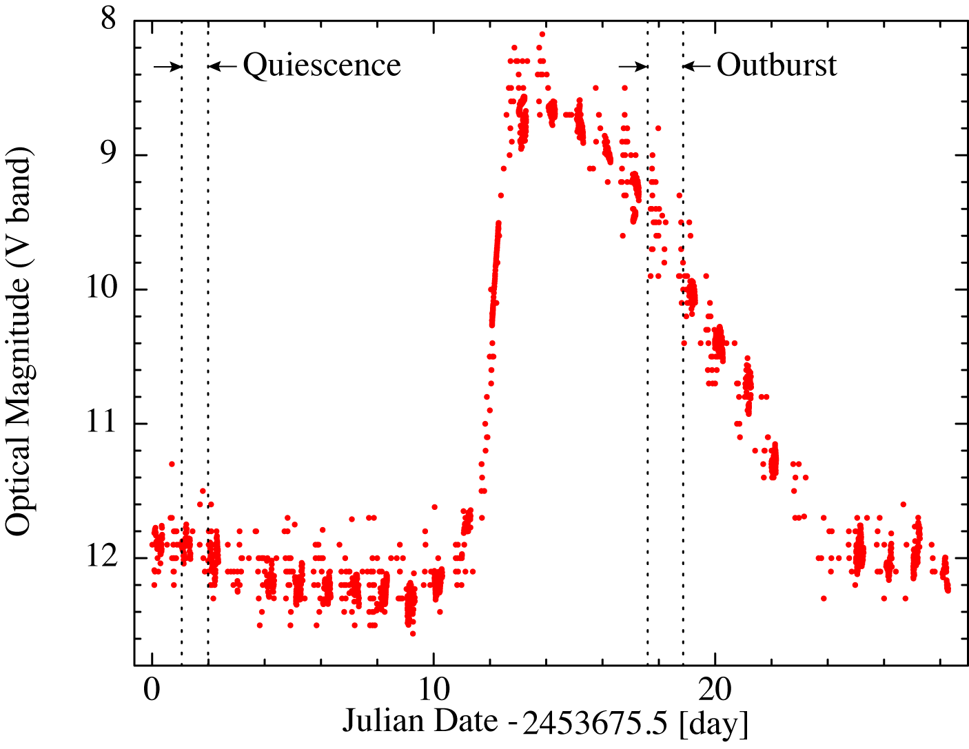
Figure 1: A V-band light curve of SS Cyg covering the Suzaku observations. The observation periods of quiescence and outburst are segmented with dashed vertical lines. Taken from the AAVSO home page.

Table 1: Suzaku observation log of SS Cyg

State	Seq. #	Observation Date	Pointing	Detector	Mode	Exp.	Intensity
		[UT]			[ks]	[c s-1]
Quiescence	40006010	2005 Nov. 02 01:02 — 02 23:39	XIS nom.	FI	Normal	39.3	3.308$\pm$0.005
				BI	Normal	39.3	4.480$\pm$0.011
				PIN	Normal	27.0	0.163$\pm$0.005
Outburst	40007010	2005 Nov. 18 14:15 — 19 20:45	XIS nom.	FI	Normal	56.0	1.580$\pm$0.003
				BI	Normal	56.0	2.427$\pm$0.007
				PIN	Normal	47.9	0.028$\pm$0.003
FI: Frontside-Illuminated CCD (XIS0, 2, 3), BI: Backside-Illuminated CCD (XIS1), PIN: HXD PIN detector. Exposure time after data screening. Intensity in the 0.4–10 keV (FI and BI CCDs) and 12–40 keV bands (PIN) with a 1$\sigma$ statistical errors. The systematic error of the PIN background (5% of the NXB) is 0.024 c s-1 in this band.

Throughout the observations, XIS was operated in the normal 5$\times$5 and 3$\times$3 editing modes during the data rate SH/H and M/L, respectively, with no window/burst options, while the HXD PIN was operated with the bias voltage of 500 V for all the 64 modules. We do not use the HXD GSO data, because we did not receive any significant signal from SS Cyg throughout. The source was placed at the XIS nominal position in both observations where the observation efficiency of all the XRTs are more than 97% of maximum throughput (Serlemitsos et al., 2007). As already known from previous observations (e.g.Wheatley et al. (2003)) the hard X-ray flux was smaller in outburst than in quiescence.

2.2 Data screening

In data reduction, we use event files that are created with the pipeline processing software (revision 1.2.2.3), and the analysis software package HEASOFT (version 6.1.3). For the XIS, we selected the events with grades 0, 2, 3, 4, and 6. We do not use bad pixels or columns where charge transfer efficiency is too low to detect/transfer X-ray signals. We also discarded the data taken during time intervals of maneuvers, low data rate, passage of SAA (South Atlantic Anomaly), the field of view being occulted by the earth or watching bright earth rim, and the pointing position being away from the source by more than $\timeform{1^{\prime}.5}$. Finally, the cleaned event files are created by removing hot/flickering pixels. In addition to the criteria described above, we accept the data without telemetry saturation. After these data selection, we combined the data of 3$\times$3 and 5$\times$5 editing modes before starting analysis. Resultant exposure time is 39.3 ks and 56.0 ks in quiescence and outburst, respectively. For creating a cleaned event file for the HXD PIN, on the other hand, we further removed the time interval during cut-off rigidity is less than 6 GeV c^-1.

In extracting photons from the source with the XIS, we take a circular integration region with a radius of 250 pixels ($\timeform{4.^{\prime}34}$) centered at the source, which includes more than 96 % of the X-ray events, while an annulus with an outer radius of 432 pixels ($\timeform{7.^{\prime}50}$) around the source region is adopted for the background-integration region. In view of statistics, we took the area of the background-integration region twice as large as that of the source-integration region. For the HXD-PIN, on the other hand, we accumulate a non-X-ray background (NXB) spectrum from a simulated NXB event file published by the HXD team. In addition to the NXB, we need to consider the cosmic X-ray background (CXB), for which we adopt the empirical model spectrum constructed on the basis of the HEAO observations (Boldt, 1987),

$$f_{\rm CXB}(E) = 9.0\times\left(\frac{E}{3~{}{\rm keV}}\right)^{-0.29}\times\exp\left(-\frac{E}{40~{}{\rm keV}}\right)\quad{\rm erg~{}cm^{-2}~{}str^{-1}~{}keV^{-1}},$$ (1)

and create a CXB spectrum from this model by the fakeit command in the spectral fit software XSPEC (Arnaud, 1996) with an exposure time of 1 Ms. In doing this, we adopt the PIN flat sky response. The background spectrum for the PIN is created by combining the NXB and CXB spectra using the mathpha command in the FTOOLS package. Since the CXB level is $\sim$5% of the NXB level, we ignore sky-to-sky variation of the CXB. The counting rates listed in table 1 are those after all the data screening described in this section are applied.

2.3 Light Curves

We show energy-resolved and background-subtracted light curves of SS Cyg in quiescence and outburst in Fig. 2.

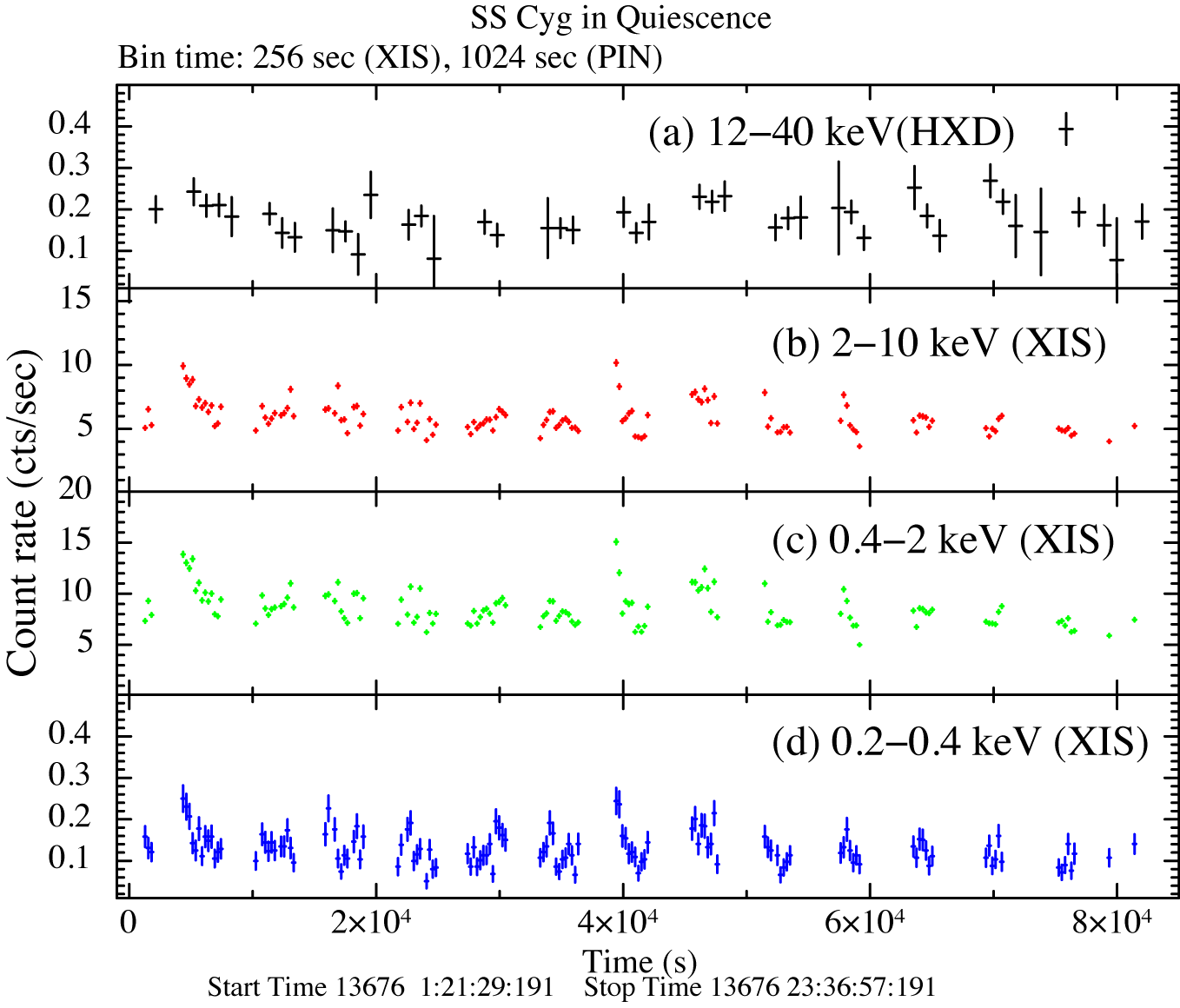
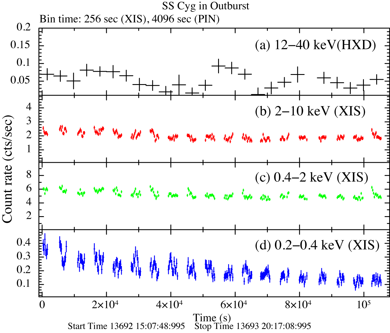
Figure 2: Background-subtracted light curves of SS Cyg in quiescence (left) and outburst (right) in the bands (a) 12–40 keV, (b) 2–10 keV, (c) 0.4–2 keV, and (d) 0.2–0.4 keV. Data from all the XIS modules are combined to make the light curves in the panels (b) through (d). The bin size of the XIS is 256 sec both in quiescence and outburst whereas that of the HXD PIN is 1024 sec in quiescence and 4096 sec in outburst. The origin of time is MJD 57676 01:23:49 and MJD 57692 14:56:10, respectively.

The source and background photons are accumulated using the integration regions explained in § 2.2. The data from the four XIS modules are combined to generate the light curves in the three energy bands 0.2–0.4 keV, 0.4–2.0 keV, and 2.0–10.0 keV. The light curve of the HXD (PIN) is created in the energy range 12–40 keV where the sensitivity of HXD becomes the maximum. The mean counting rates are summarized in table 1. In outburst, the average intensity in the 12-40 keV band is 5.9% of the NXB intensity of the PIN, whereas there remains 5% systematic error in the NXB model intensity. Hence, the detection of the PIN in outburst is marginal. In the energy bands above 0.4 keV, the source is brighter in quiescence than in outburst, as demonstrated by Wheatley et al. (2003), and is more variable. The flux below 0.4 keV is, on the other hand, higher in outburst. Moreover, the source obviously declines throughout the observation, whereas the intensity is nearly constant in the higher energy bands. These facts suggest that Suzaku detected high energy end of the emission from the optically thick BL which appears in outburst (Tylenda, 1977; Pringle, 1977; Pringle & Savonije, 1979; Patterson & Raymond, 1985; Wheatley et al., 2003).

2.4 Average spectra

In Fig. 3, we show averaged spectra of SS Cyg from the XIS and the HXD-PIN in quiescence and outburst.

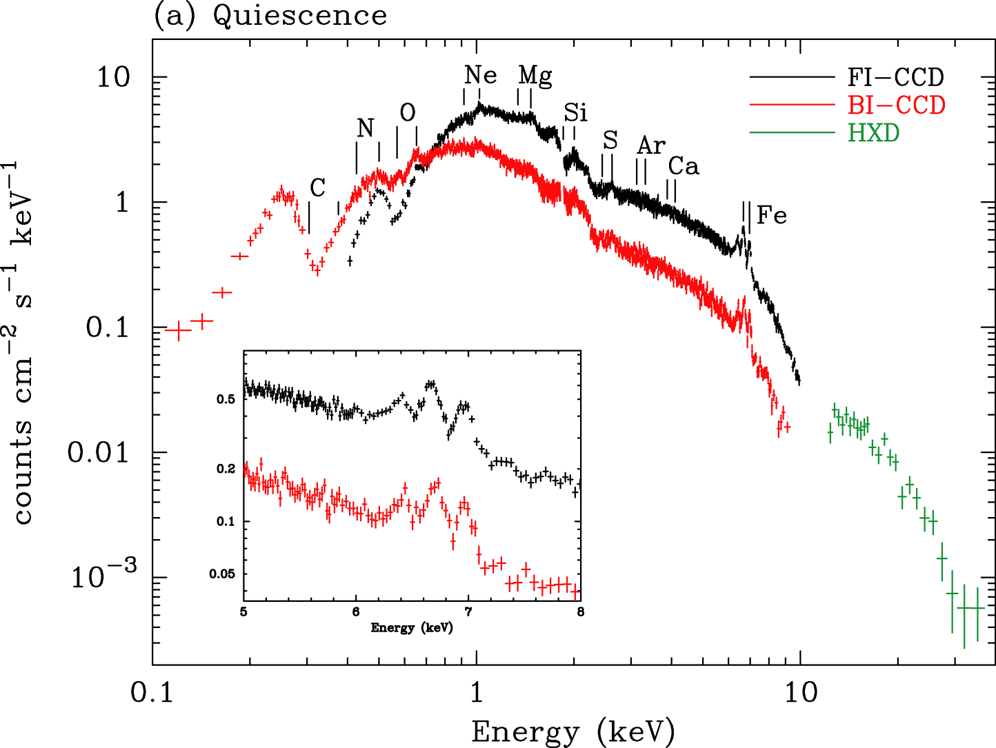
Figure 3: Averaged spectra of SS Cyg in quiescence and outburst. The source and background integration regions are explained in § 2.2. The data from XIS0, 2, and 3 are combined into a single FI-CCD spectrum whereas BI-CCD spectrum originates from XIS1. The insets are the blowups in the 5-8 keV band showing profiles of iron K$\alpha$ emission lines.

The source and background photons are accumulated using the integration regions explained in § 2.2. The data from XIS0, 2, and 3 are combined into a single FI-CCD spectrum. The BI-CCD spectrum originates solely from the XIS1 data.

SS Cyg is detected at least up to $\sim$30 keV with the HXD-PIN in quiescence, whereas the detection of the PIN in outburst is marginal as noted in § 2.3. From the inset, iron K$\alpha$ emission lines are clearly resolved into 6.4, 6.7, and 7.0 keV components. The 6.4 keV line indicates reflection of the hard X-ray emission from the white dwarf and possibly from the accretion disk, as pointed out by Done & Osborne (1997). Note that the 6.4 keV line is broad in outburst. Except for the iron emission lines, only weak signs of H-like K$\alpha$ lines are visible from the other elements in quiescence. The outburst spectra, on the other hand, are softer than those in quiescence, and are characterized by H-like and He-like K$\alpha$ emission lines from nitrogen to iron (Okada et al., 2008). From the inset, the He-like iron K$\alpha$ line at 6.7 keV is much stronger than the H-like line at 7.0 keV, in contrast to the quiescence spectra. These facts indicate that the plasma has a temperature distribution, and that the average plasma temperature is significantly lower in outburst than in quiescence. The decaying soft component in the light curves (Fig. 2) appears as an excess soft emission below $\sim$0.3 keV in the BI-CCD spectrum in outburst.

3 Analysis and Results

3.1 Spectral components and their models

In Fig. 4, we show schematic view of spectral ingredients of SS Cyg in the 0.2–40 keV band.

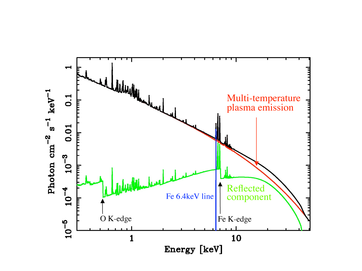
Figure 4: Schematic view of the spectral component of SS Cyg in the 0.2–40 keV band.

This picture is originally proposed by Done & Osborne (1997) on the basis of their analysis of the Ginga and ASCA data of SS Cyg. The hard spectrum of SS Cyg is primarily composed of an optically thin thermal plasma emission with a temperature distribution (§ 2.4), for which Done & Osborne (1997) introduced a power-law type differential emission measure (DEM) model as

$$d({\rm EM})\propto\left(\frac{T}{T_{\rm max}}\right)^{\alpha}\,d(\log T)\propto\left(\frac{T}{T_{\rm max}}\right)^{\alpha-1}\,dT,$$ (2)

where $T_{\rm max}$ is the maximum temperature of the plasma. The model they used, named cevmkl in XSPEC, is an optically thin thermal plasma emission model (mekal in XSPEC, Mewe et al. (1985, 1986); Liedahl et al. (1995); Kaastra et al. (1996)) convoluted with this temperature distribution. Since it can successfully represent $\sim$30 spectra of the dwarf novae (Baskill et al., 2005) observed with ASCA, we adopt this model as well in this paper. In addition to this main component, its reflection from the white dwarf (and the accretion disk) occupies significant fraction of the observed X-ray flux, as required from detection of a fluorescent iron K$\alpha$ line at 6.4 keV. To represent the reflection, we adopt the model reflect (Magdziarz & Zdziarski, 1995), which is a convolution-type model describing reflectivity of neutral material. In summary, the X-ray spectra of SS Cyg are composed of the multi-temperature optically thin thermal plasma component, its reflection from the white dwarf (and the accretion disk), and the fluorescent iron emission line at 6.4 keV.

3.2 Evaluation of plasma parameters

Our purpose is to constrain the geometry of the optically thin thermal plasma in SS Cyg. In doing this, we can utilize the equivalent width (EW) and the profile of the 6.4 keV emission line. The EW reflects a covering fraction of a reflector viewed from the plasma (Makishima, 1986). The profile contains information of motion of the reflector. From continuum analysis, the covering fraction of the reflector can independently be evaluated.

To utilize these methods, however, it is essential to know a priori the iron abundance $Z_{\rm Fe}$. For its estimation, we generally make use of the relative intensities and the EWs of the He-like and H-like iron K$\alpha$ emission lines at 6.7 keV and 7.0 keV, respectively. In deriving $Z_{\rm Fe}$ from these quantities, we need to know the plasma emission parameters such as $T_{\rm max}$ and $\alpha$ through spectral fitting of the cevmkl model to the observed data. One may suspect that it is enough to fit the spectrum containing the He-like and H-like lines locally with a single temperature optically thin thermal plasma model. This does not work properly, however, since the temperature of the plasma in SS Cyg is distributed in such a wide range, from $T_{\rm max}\simeq 20$ keV (see below) down to $\sim$0.1 keV indicated by the nitrogen and oxygen lines, that plasma emission components whose temperatures are too high enhance only the continuum level and dilute the iron emission lines, thereby resulting in a lower abundance estimation (Done & Osborne, 1997).

To know the plasma emission parameters $T_{\rm max}$ and $\alpha$, however, we need to know the metal abundances, the iron abundance ($Z_{\rm Fe}$) in particular and the oxygen abundance ($Z_{\rm O}$) as well, and the covering fraction of the reflector ($\Omega$), because they couple with each other in the spectrum above 7 keV. At this stage, we have found that the plasma emission parameters ($T_{\rm max}$ and $\alpha$) and the reflection parameters ($\Omega$, $Z_{\rm Fe}$ and $Z_{\rm O}$) depend on each other, and need to determine them in a self-consistent manner. Accordingly, we carried out a combined spectral fit among the quiescence and outburst spectra in selected bands crucial to determine $T_{\rm max}$, $\alpha$, $\Omega$, $Z_{\rm Fe}$, and $Z_{\rm O}$. They are the quiescence spectra in the 4.2–40 keV band (sensitive to $T^{\rm Q}_{\rm max}$, $\alpha^{\rm Q}$, $Z_{\rm Fe}$, and $\Omega^{\rm Q}$), the outburst spectra in the 4.2–10 keV (sensitive to $T^{\rm O}_{\rm max}$, $\alpha^{\rm O}$, $Z_{\rm Fe}$, and $\Omega^{\rm O}$) and that in 0.55–0.72 keV bands (sensitive to $Z_{\rm O}$ and $\alpha^{\rm O}$), where the superfixes ‘Q’ and ‘O’ indicate quiescence and outburst, respectively. We ignore the intermediate 0.72–4.2 keV band in outburst, because (1) this band is of no use to evaluate the parameters listed above. Including this band may rather introduce unexpected systematic errors in the parameters of interest, (2) this band includes the emission lines from Ne to Ca whose abundances are uncertain until we determine $T^{\rm O}_{\rm max}$ and $\alpha^{\rm O}$, and (3) as will be found later in table 2 and 3, values of $\alpha^{\rm O}$ are different for different elements. The entire outburst spectrum can not be fit with a single $\alpha$ cevmkl model. We set $T_{\rm max}$, $\alpha$, and $\Omega$ free to vary in quiescence and outburst separately, because the geometry of the plasma, and hence its temperature distribution may be different, whereas we set $Z_{\rm Fe}$ and $Z_{\rm O}$ common between quiescence and outburst. Note that we do not use the PIN spectrum in outburst, because the detection is marginal due to the NXB uncertainty (§ 2.3 and 2.4). The result of the fits is shown in Fig. 5, and its best-fit parameters are summarized in table 2.

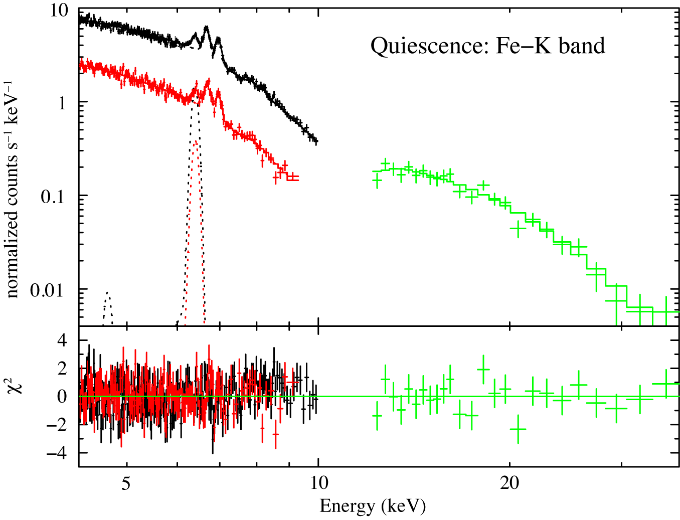
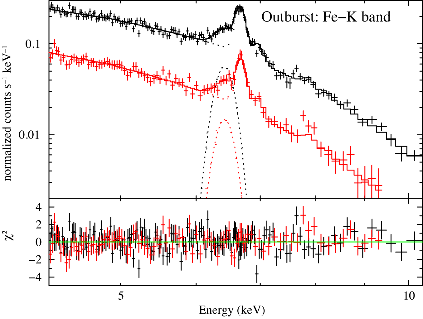
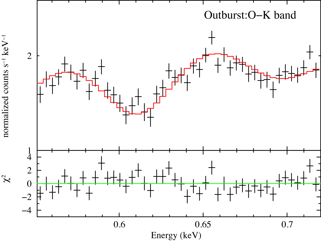
Figure 5: Result of the simultaneous fits of the cevmkl plus reflection model to the 4.2–40 keV band in quiescence, the 4.2–10 keV and 0.55–0.72 keV bands in outburst. Black, red, and green colors are used for the data and the model of the FI-CCD, BI-CCD, and PIN, respectively, except for the outburst 0.55–0.72 keV spectrum where only the BI-CCD data are utilized.

Table 2: Best-fit parameters of the simultaneous fit of the cevmkl plus reflection model to the quiescence and outburst spectra.

Phase	Quiescence	Outburst
Energy band [keV]	4.2–40	4.2–10	0.55–0.72
$T_{\rm max}$∗ [keV]	$20.4^{+4.0}_{-2.6}\,(\pm 3.0)$	$6.0^{+0.2}_{-1.3}$
$\alpha$†	$0.7^{+0.3}_{-0.1}\,(\pm 0.1)$	$5.8^{+2.6}_{-1.4}$	$-0.36^{+0.02}_{-0.03}$
$\Omega/2\pi$‡	$1.7\pm 0.2\,(\pm 0.1)$	$0.9^{+0.5}_{-0.4}$
$Z_{\rm Fe}$§	$0.37^{+0.01}_{-0.03}\,(\pm 0.01)$
$Z_{\rm O}$∥	$0.46^{+0.04}_{-0.03}\,(\pm 0.01)$
$\chi^{2}$ (d.o.f.)	728.2 (657)
Note — Errors in parentheses are systematic errors associated with the NXB uncertainty of the HXD-PIN. Maximum temperature of the optically thin thermal plasma. Power of DEM as $d({\rm EM})\propto(T/T_{\rm max})^{\alpha-1}dT$. Solid angle (covering fraction) of the reflector viewed from the plasma. Iron abundance in a unit of solar. Constrained to be common among the three energy bands. The solar abundance table of Anders & Grevesse (1989) is adopted, in which [Fe/H] = $4.68\times 10^{-5}$. Oxygen abundance in a unit of solar. Constrained to be common among the three energy bands. The solar abundance table of Anders & Grevesse (1989) is adopted, in which [O/H] = $8.51\times 10^{-4}$.

The fits are marginally acceptable at the 90% confidence level. The parameters of the plasma and the reflector are determined consistently between quiescence and outburst with unprecedented precision. We adopt Anders & Grevesse (1989) as the solar abundances of the metals. The DEM power $\alpha$ is varied independently between the iron and oxygen bands in the outburst spectra, because the cooling functions are significantly different between these two bands (Gehrels & Williams, 1993). In fact, the resultant $\alpha$ values are significantly different between O ($\simeq-0.4$) and Fe ($\sim$6). Considering this large difference, we have checked mutual consistency of the model spectra in the two energy bands in outburst. The result is shown in Fig. 6.

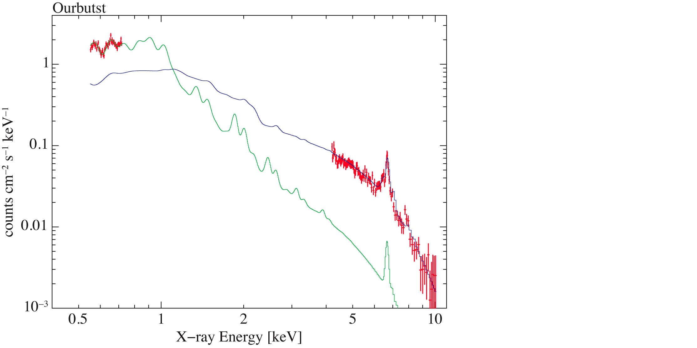
Figure 6: The outburst spectra and the models used to determine the parameters of the plasma emission and the reflection. Only the data of the XIS1 are shown for clarity in red. The green and the blue curves show the best-fit models in the 0.55–0.72 keV and 4.2-40 keV bands, respectively, whose parameters are summarized in table 5.

The extrapolation of the best-fit model in one band does not exceed the observed flux in the other band. Hence, the fits to the two energy bands in outburst are revealed to be mutually consistent. The maximum temperature of the plasma in quiescence ($T^{\rm Q}_{\rm max}=20.4^{+4.0}_{-2.6}$ keV) is significantly higher than that in outburst ($T^{\rm O}_{\rm max}=6.0^{+0.2}_{-1.3}$ keV). Our $T^{\rm Q}_{\rm max}$ is consistent with that of Done & Osborne (1997) ($=21^{+11}_{-5.7}$ keV). Their $T^{\rm O}_{\rm max}$ ($=9.6^{+3.4}_{-1.7}$ keV) seems slightly higher than ours, though this may be due to different outburst phases at which the observations were carried out. The optically thin thermal plasma is covered with the reflector more in quiescence ($\Omega^{\rm Q}/2\pi=1.7\pm 0.2$) than in outburst ($\Omega^{\rm O}/2\pi=0.9^{+0.5}_{-0.4}$). The covering fractions are not constrained by Done & Osborne (1997) very well ($\Omega^{\rm Q}/2\pi=0.6^{+1.1}_{-0.6}$ and $\Omega^{\rm O}/2\pi=2.2^{+1.8}_{-1.5}$). The iron and oxygen abundances are both sub solar ($Z_{\rm Fe}=0.37^{+0.01}_{-0.03}Z_{\odot}$ and $Z_{\rm O}=0.46^{+0.04}_{-0.03}Z_{\odot}$).

Finally, we have considered the effects of the 5% systematic PIN NXB error. We have made background spectra of the PIN with an intensity being enhanced or reduced by 5%, subtracted them from the quiescence PIN spectrum, and repeated the combined spectral fit described above. The resultant systematic errors are summarized in parentheses in table 2. We have found $T^{\rm Q}_{\rm max}$ is accompanied by the largest fractional systematic error of $\pm$3.0 keV. Fortunately, those of the other parameters are smaller than the statistical ones. Since we do not use the outburst PIN data, there appears no systematic error in $T^{\rm O}_{\rm max}$, $\alpha^{\rm O}$, and $\Omega^{\rm O}/2\pi$.

3.3 Abundance of the other elements

We can identify He-like and H-like K$\alpha$ emission lines from nitrogen to iron in the outburst spectra shown in Fig. 3. Utilizing the intensities of these lines, we can estimate the abundances of corresponding elements. The line intensities depend upon $T^{\rm O}_{\rm max}$, $\alpha^{\rm O}$, and the abundance. Among them, We have constrained $T^{\rm O}_{\rm max}$ well by the combined fit analysis described in § 3.2. With $T^{\rm O}_{\rm max}$ being fixed at 6.0 keV (table 2), we have evaluated the abundances by fitting the cevmkl model to the K$\alpha$ lines of each element separately. In principle, $\alpha^{\rm O}$ (see eq. (2)) is determined by the relative intensities of the He-like and H-like K$\alpha$ lines, and the abundance is constrained by and their EWs. The results of the fits are shown in Fig. 7 and the best-fit abundances as well as $\alpha^{\rm O}$ are summarized in table 3.

Table 3: Summary of the abundances of iron, calcium, argon, sulfur, silicon, magnesium, neon, oxygen, and carbon.

Element	Energy Band	$N_{\rm H}$	$T^{\rm O}_{\rm max}$	$\alpha^{\rm O}$	Abundance	${\rm\chi^{2}}$ (d.o.f.)	${\rm\chi^{2}_{\nu}}$
	(keV)	($10^{19}$cm-2)	(keV)		(${\rm Z_{\odot}}$)
Fe	4.2–10	${\rm 5.0^{f}}$	$6.0^{+0.2}_{-1.3}$	${\rm 5.8^{+2.6}_{-1.4}}$	${\rm 0.37^{+0.01}_{-0.03}}$	728.3 (657)	1.11
Ca	2.8–5.0	${\rm 5.0^{f}}$	${\rm 6.0^{f}}$	${\rm 2.2^{+0.5}_{-0.4}}$	${\rm 0.73^{+0.35}_{-0.36}}$	263.7 (265)	1.00
Ar					${\rm 0.93^{+0.34}_{-0.32}}$
S	2.15–3.0	${\rm 5.0^{f}}$	${\rm 6.0^{f}}$	${\rm 0.72^{+0.16}_{-0.14}}$	${\rm 0.88\pm{0.09}}$	242.1 (171)	1.42
Si	1.6–2.3	${\rm 5.0^{f}}$	${\rm 6.0^{f}}$	${\rm 0.88^{+0.15}_{-0.13}}$	${\rm 0.90\pm{0.07}}$	389.0 (244)	1.59
Mg	1.2–1.7	${\rm 5.0^{f}}$	${\rm 6.0^{f}}$	${\rm 0.44\pm 0.06}$	${\rm 0.80\pm 0.06}$	316.2 (267)	1.19
Ne	0.8–1.2	${\rm 5.0^{f}}$	${\rm 6.0^{f}}$	${\rm 0.31\pm 0.02}$	${\rm 0.49\pm 0.04}$	429.8 (217)	1.99
fit with the BI spectrum only
O	0.55–0.72	${\rm 5.0^{f}}$	$6.0^{+0.2}_{-1.3}$	${\rm-0.36^{+0.02}_{-0.03}}$	${\rm 0.46^{+0.04}_{-0.03}}$	728.3 (657)	1.11
N	0.3–0.52	${\rm 3.5^{f}}$	${\rm 6.0^{f}}$	${\rm 0.68^{+0.20}_{-0.23}}$	${\rm 0.40^{+0.99}_{-0.40}}$	44.7 (49)	0.91
C					${\rm 3.47^{+1.60}_{-0.99}}$
N	0.3–0.52	${\rm 5.0^{f}}$	${\rm 6.0^{f}}$	${\rm 0.64^{+0.17}_{-0.22}}$	${\rm 0.30^{+0.97}_{-0.30}}$	44.6 (49)	0.91
C					${\rm 3.20^{+1.41}_{-0.90}}$
N	0.3–0.52	${\rm 7.9^{f}}$	${\rm 6.0^{f}}$	${\rm 0.56^{+0.10}_{-0.22}}$	${\rm 0.13^{+0.94}_{-0.13}}$	44.6 (49)	0.91
C					${\rm 2.76^{+1.14}_{-0.76}}$
Note.— ‘f’ implies the parameter is fixed. Fixed at 6.0 keV obtained from the simultaneous fit (table 2 in § 3.2). Fixed at ${\rm 5.0\times 10^{19}~{}cm^{-2}}$ obtained from the Chandra LETG observation (Mauche, 2004). The same values as summarized in table 2.

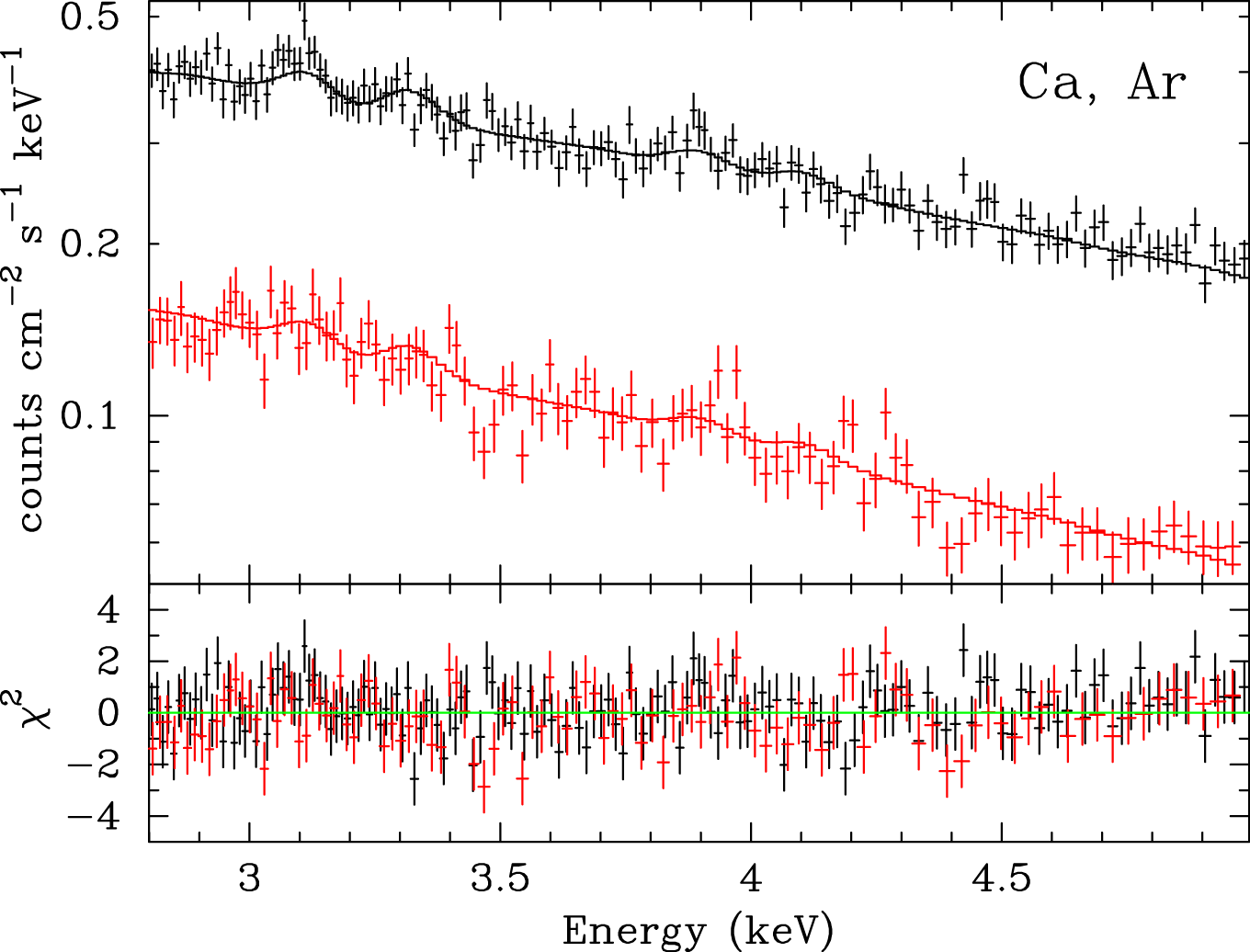
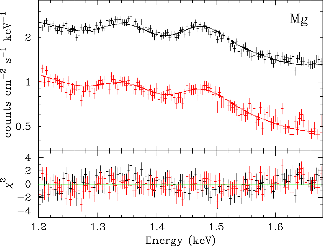
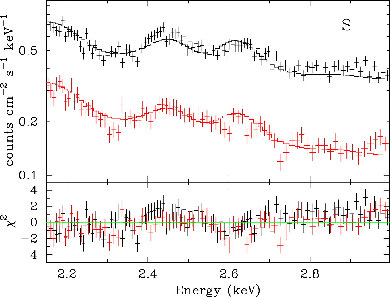
Figure 7: Local cevmkl fits to the He-like and H-like K$\alpha$ emission lines of Ca, Ar, S, Si, Mg, Ne, N, and C. The upper panel shows the data (crosses) and the models (histograms), while the lower panel shows the residuals in a unit of the standard deviation. In order to show detection of the C emission lines, we have also plotted a cevmkl model with the C abundance being set equal to zero as a dotted histogram in panel (f).

The spectral fit is started from a higher energy band. This is because the line emissions from lighter elements do not affect the determination of the abundances of heavier elements, whereas L-shell emission from the heavier elements is possible to affect the fit to the lighter element lines. As the abundances of the heavier elements have been measured, those of the lighter elements are determined one after the other by fixing the abundances of the heavier elements at their best-fit values. The fit to Ca and Ar is carried out simultaneously, and so is to N and C. Note that only BI-CCD is used for the fit to N and C.

In order to estimate the abundances of N and C, we have to take into account several possible systematic effects such as the low energy response of the XIS, the uncertainty of the contamination accumulating on the optical blocking filters above the CCD chips, and systematic error of the hydrogen column density to SS Cyg. Among them, the low energy response and the contamination are investigated by ourselves with the PKS 2155–304 data taken during Nov. 30 – Dec. 2, 2005, which date is close enough to our SS Cyg observations. As summarized in Appendix A, we need to apply additional carbon K-edge with $\tau=0.88\pm 0.05$ and extra $N_{\rm H}=8.2\pm 0.7\times 10^{19}$ cm^-2. By applying these corrections to the model, we can utilize the BI-CCD data down to 0.23 keV. In order to estimate the $N_{\rm H}$ systematic error, on the other hand, we have checked variation of the best-fit parameters with an $N_{\rm H}$ of 3.5, 5.0, and 7.9$\times 10^{19}$ cm^-2. These values are selected based on $N_{\rm H}=5.0^{+2.9}_{-1.5}\times 10^{19}$ cm^-2 obtained from the Chandra LETG observation of SS Cyg in outburst (Mauche, 2004). Since the H-like K$\alpha$ line of C and the He-like K$\alpha$ line of N cannot be resolved with the BI-CCD energy resolution, we employ the BI-CCD spectrum in the 0.3–0.52 keV band covering the emission lines of both C and N, and fit cevmkl model.

We remark that not all the fits shown in Fig. 7 are acceptable. The fit to Si is especially poor. As evident from the fit residuals inconsistent between the BI and FI-CCDs at around the Si K-edge (1.7–1.9 keV), this is mainly due to systematic error associated with energy response calibration. Nevertheless, the best-fit parameters summarized in table 3 indicate that the abundances of the medium-Z elements (Si, S, and Ar) are close to solar ones, whereas they are reduced for both lighter and heavier elements. The exception is the carbon abundance whose lower limit is 2.0$Z_{\odot}$ even if we consider the systematic error of $N_{\rm H}$. Since the energy resolution of the XIS in the C line energy band is not so good as in higher energy band, we have drawn the cevmkl model with the C abundance being set equal to zero in Fig. 7(f) as the dotted histogram. The data excess associated with the C emission is clear.

Given the spectral parameters, we can calculate X-ray fluxes of SS Cyg, which is $19.5\times 10^{-11}$ erg cm^-2 s^-1 and $8.1\times 10^{-11}$ erg cm^-2 s^-1 in the 0.4–10 keV band in quiescence and outburst, respectively. Assuming the distance of 166 pc (Harrison et al., 1999), we obtain the luminosities of $6.4\times 10^{32}$ erg s^-1 and $2.7\times 10^{32}$ erg s^-1, respectively, in this energy band.

3.4 Iron emission lines

3.4.1 Quiescence

In order to constrain the geometry of the optically thin thermal plasma in quiescence, we have attempted to evaluate the parameters of the 6.4 keV line in detail. We fit a model composed of a power-law continuum and three narrow Gaussian lines at 6.4 keV, 6.7 keV and 7.0 keV to the XIS spectra in the 5–9 keV band. The result of the fit is shown in Fig. 8 and the best-fit parameters are summarized in table 4.

Table 4: Best-fit parameters of the iron K$\alpha$ emission lines with the 5–9 keV XIS spectra in quiescence.

Component	Parameter	3 lines	4 lines
Continuum	$\Gamma$	$1.60^{+0.03}_{-0.02}$	$1.62^{+0.02}_{-0.03}$
	$N_{\rm C}$	$9.13\pm 0.07$	$9.50\pm 0.08$
H-like line	$E_{\rm L}$ (keV)	$6.968^{+0.003}_{-0.008}$	$6.966^{+0.006}_{-0.008}$
	$N_{\rm L}$	$5.30^{+0.39}_{-0.41}$	$5.39^{+0.38}_{-0.42}$
	$\sigma$ (keV)	0 (fixed)	0 (fixed)
	EW (eV)	$130^{+9}_{-10}$	$132^{+9}_{-10}$
He-like line	$E_{\rm L}$ (keV)	$6.682^{+0.002}_{-0.008}$	$6.684^{+0.004}_{-0.006}$
	$N_{\rm L}$	$7.81^{+0.41}_{-0.42}$	$7.67^{+0.36}_{-0.48}$
	$\sigma$ (keV)	0 (fixed)	0 (fixed)
	EW (eV)	$181\pm 10$	$175^{+8}_{-11}$
Fluorescence line parameters
Narrow line	$E_{\rm L}$ (keV)	$6.407^{+0.008}_{-0.011}$	$6.404^{+0.012}_{-0.008}$
	$N_{\rm L}$	$4.02^{+0.37}_{-0.36}$	$2.46^{+0.91}_{-0.38}$
	$\sigma$ (keV)	0 (fixed)	0 (fixed)
	EW (eV)	$86\pm 8$	$53^{+20}_{-9}$
Broad line	$N_{\rm L}$	—	$2.38^{+0.98}_{-0.50}$
	$\sigma$ (keV)	—	$0.112^{+0.055}_{-0.031}$
	EW (eV)	—	$51^{+21}_{-11}$
	$\chi^{2}$ (d.o.f)	261.7 (233)	251.5 (231)
	$\chi^{2}_{\nu}$	1.12	1.09
Line central energy. The value is constrained to be the same between the narrow and broad 6.4 keV components. Continuum normalization in a unit of $10^{-3}$ cm-2 keV-1 s-1 at 1 keV. Line normalization (intensity) in a unit of $10^{-5}$ photons cm-2 s-1. Equivalent width. Photon index.

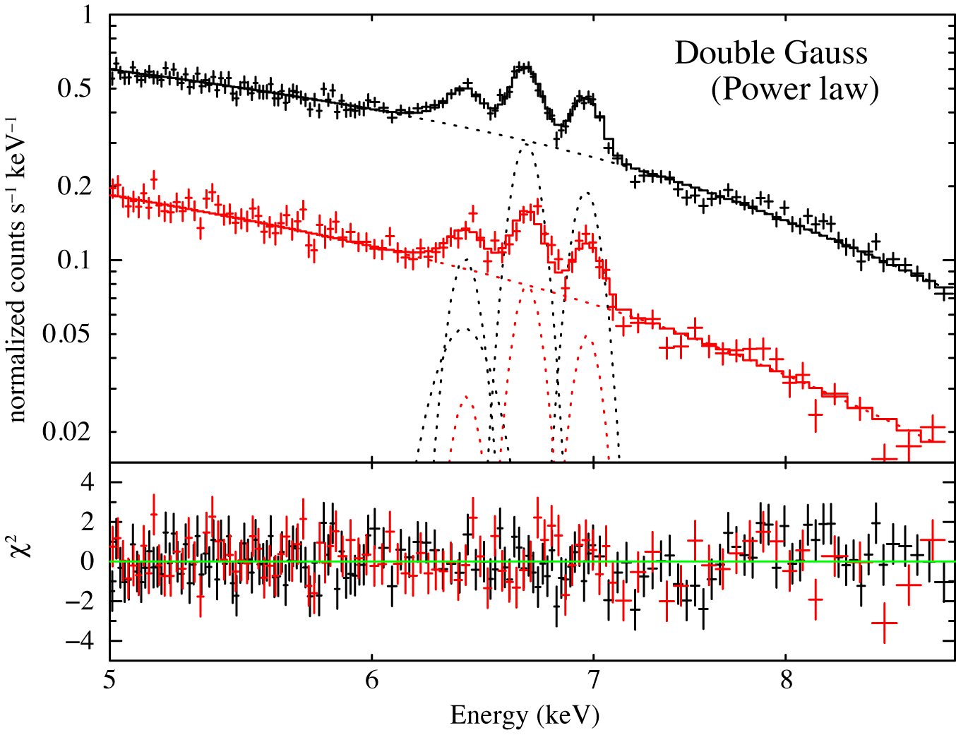
Figure 8: Fits of a power law plus 3 Gaussians (left) and 4 Gaussians (right) to the 5–9 keV XIS spectra in quiescence.

There remains a slight excess emission in the low energy tail of the 6.4 keV line. We thus have added a broad Gaussian to the 6.4 keV line. The results are also summarized in table 4 and Fig. 8. The fit is improved with a $\chi^{2}$ (d.o.f) value from 261.7 (233) to 251.5 (231). The chance probability for this to occur is 0.009, which implies adding a broad Gaussian is significant at $\sim$99% confidence level. The resultant equivalent width of the narrow and broad lines is ${\rm EW\,(narrow)}=53^{+20}_{-9}$ eV and ${\rm EW\,(broad)}=51^{+21}_{-11}$ eV.

3.4.2 Outburst

In outburst, the 6.4 keV line is obviously broad (Fig. 3). We therefore adopt a broad Gaussian for modeling the 6.4 keV emission line. As in the case of the fit to the quiescence spectra (§ 3.4.1), we have tried to fit a model composed of a power law and three Gaussians to the XIS spectra in the 5–9 keV band. The result is shown in Fig. 9, and the best-fit parameters are summarized in table 5.

Table 5: Best-fit parameters of the iron K$\alpha$ emission lines with the 5–9 keV XIS spectra in outburst.

Component	Parameter
Continuum	$\Gamma$	$2.16^{+0.09}_{-0.05}$
	$N_{\rm C}$	$6.77^{+0.65}_{-0.12}$
H-like K$\alpha$	$E_{\rm L}$ (keV)	$6.936^{+0.028}_{-0.036}$
	$N_{\rm L}$	$0.82\pm 0.17$
	$\sigma$ (keV)	0 (fixed)
	EW (eV)	$80\pm 17$
He-like K$\alpha$	$E_{\rm L}$ (keV)	$6.682^{+0.004}_{-0.007}$
	$N_{\rm L}$	$4.37^{+0.29}_{-0.30}$
	$\sigma$ (keV)	0 (fixed)
	EW (eV)	$390^{+26}_{-27}$
Neutral K$\alpha$	$E_{\rm L}$ (keV)	$6.448^{+0.024}_{-0.025}$
	$N_{\rm L}$	$2.90^{+0.95}_{-0.38}$
	$\sigma$ (keV)	$0.12^{+0.06}_{-0.03}$
	EW (eV)	$208^{+68}_{-27}$
	$\chi^{2}$ (d.o.f)	198.1 (155)
	$\chi^{2}_{\nu}$	1.28
Line central energy. The value is constrained to be the same between the narrow and broad 6.4 keV components. Continuum normalization in a unit of $10^{-3}$ cm-2 keV-1 s-1 at 1 keV. Line normalization (intensity) in a unit of $10^{-5}$ photons cm-2 s-1. Equivalent width. Photon index.

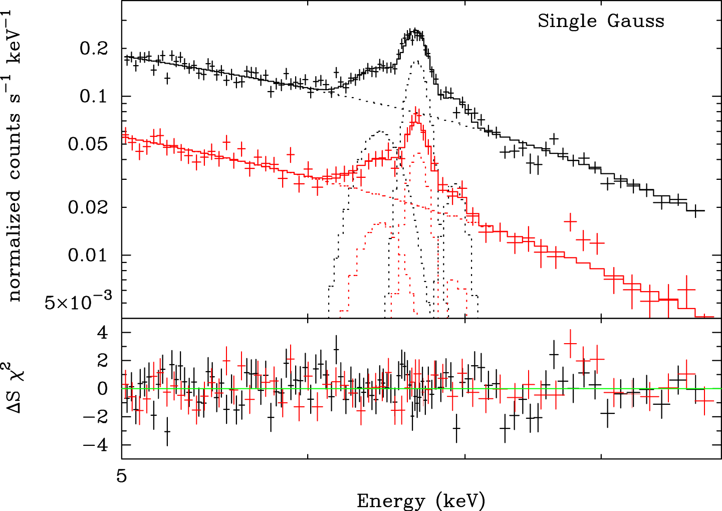
Figure 9: Fits of a power law plus 3 Gaussians to the 5–9 keV XIS spectra in outburst.

The equivalent width of the 6.4 keV line is as large as $\sim$210 eV. The energy width of the line $\sigma=0.12$ keV is nearly the same as that of the broad component in quiescence.

In quiescence, the narrow component dominates the 6.4 keV line. In order to see if there is a narrow component also in the outburst spectra, we have implemented another narrow Gaussian ($\sigma=0$) into the model at the same central energy of the broad 6.4 keV component. The fit with this model, however, only provides an upper limit to the narrow 6.4 keV line with an equivalent width of $<39$ eV, or $<20$% of the broad component.

4 Discussion

4.1 Location of the optically thin thermal plasma in quiescence

4.1.1 Geometry of the plasma

We have shown in § 3.2 that the optically thin thermal plasma in quiescence is covered with the reflector with a solid angle of $\Omega^{\rm Q}/2\pi=1.7\pm 0.2$. Such a high value of $\Omega^{\rm Q}/2\pi$ is achieved only in a limited number of high-mass X-ray binaries (e.g. Watanabe et al. (2003)) that are surrounded by matter as thick as $\sim$10²⁴ H cm^-2. The thickness of matter to SS Cyg, on the other hand, only amounts to $N_{\rm H}\lesssim 10^{20}$ cm^-2 or $\tau\lesssim 10^{-4}$ for Thomson scattering, which is too transparent to reflect X-rays efficiently. Candidates of the reflection site are therefore limited to the white dwarf and the accretion disk. The observed $\Omega^{\rm Q}/2\pi$, however, requires a special geometry, because even an infinite slab can only subtend a solid angle of $\Omega/2\pi=1$ over an X-ray source above it. The plasma should be compact enough compared to the size of the white dwarf, and should be located very close to the white dwarf and the accretion disk. We consider the standard optically thin BL (Patterson & Raymond, 1985) as the most plausible configuration of the optically thin thermal plasma in quiescence (see also Fig. 10).

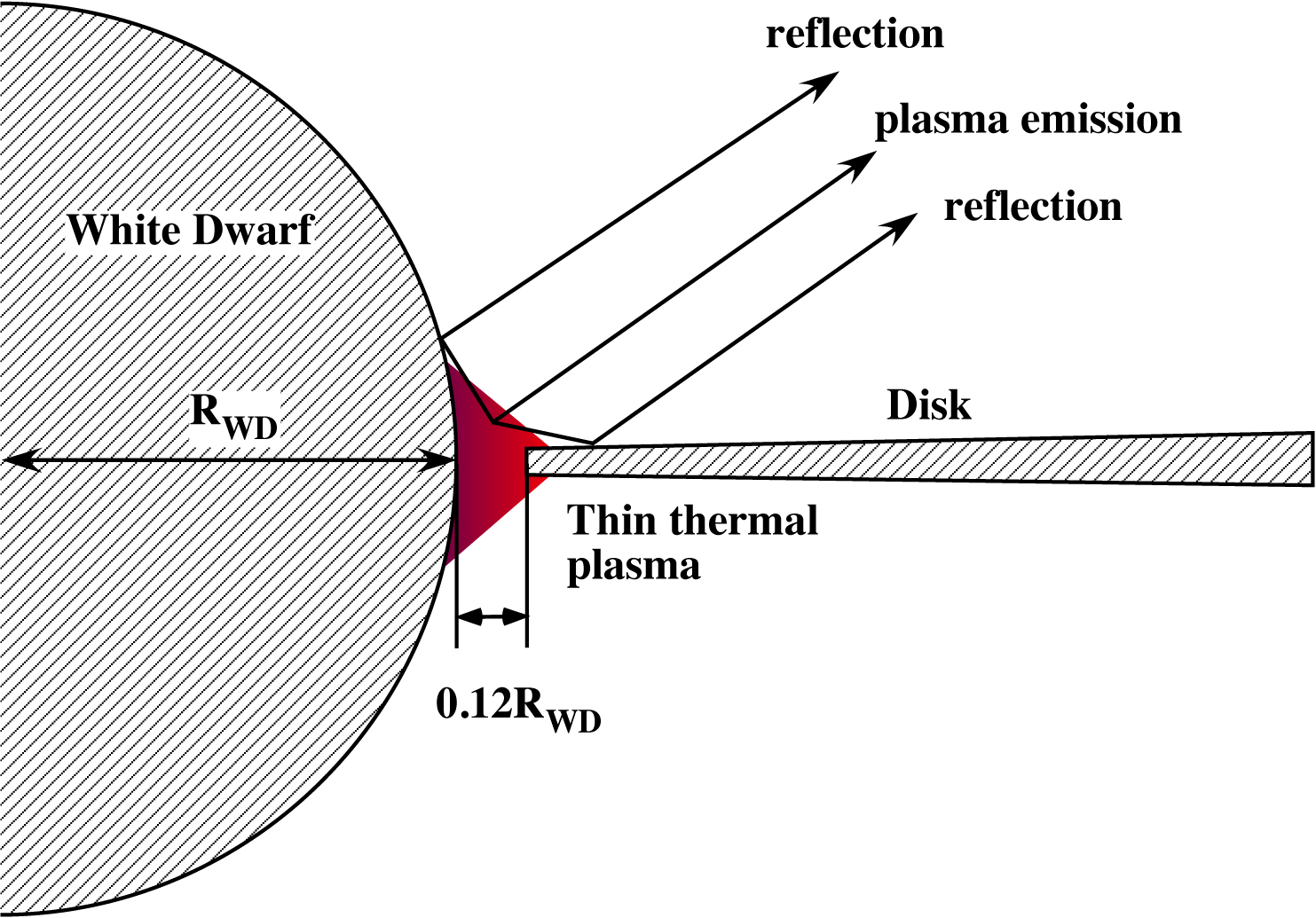
Figure 10: Geometry of the BL in quiescence deduced from the Suzaku observation.

In § 3.4.1, we have shown that the 6.4 keV iron line profile favors the broad component in addition to the narrow component, which can naturally be interpreted as originating from the accretion disk and the white dwarf, respectively, via fluorescence. The width of the broad component $\sigma=0.11^{+0.06}_{-0.03}$ keV corresponds to a line-of-sight velocity dispersion of 5300${}^{+2500}_{-1500}$ km s^-1, which is consistent with the line-of-sight Keplerian velocity amplitude of the accretion disk just on the 1.19$M_{\odot}$ white dwarf ($v_{\rm K}\sin i=$ 3800$\pm$400 km s^-1, where we set $i=37^{\circ}\pm 5^{\circ}$).

4.1.2 Size of the boundary layer

Now that we know the abundance of iron $0.37^{+0.01}_{-0.03}Z_{\odot}$ (§ 3.2), we can estimate the height of the boundary layer in quiescence on the basis of the standard BL geometry displayed in Fig. 10. George & Fabian (1991) theoretically calculated the equivalent width of the fluorescent iron K$\alpha$ line due to a point source being located above an infinite slab (i.e, $\Omega\!=\!2\pi$). The equivalent width depends on the inclination angle $i$ between the observer’s line of sight and the normal of the slab, a photon index of the spectrum of the illuminating point source, and an iron abundance of the slab. In applying their calculation to the observed narrow 6.4 keV component, we have adopted the following parameters;

1. We set the inclination angle $i\!=\!60^{\circ}$, which is the average over the visible hemisphere of the white dwarf surface (Done & Osborne, 1997).

2. The observed continuum spectra above 5 keV are represented with a power law with a photon index of $\sim$1.6 (table 4). This photon index is, however, affected by the reflected continuum. In order to correct this, we have retried a fit with a power law plus its reflection with $\Omega^{\rm Q}/2\pi$ and $Z_{\rm Fe}$ fixed at the values listed in table 2. The resultant photon index is $\Gamma=1.8$, which we adopt for the power law incident on the white dwarf surface.

With this parameter set, we have obtained an expected equivalent width of the narrow 6.4 keV iron line to be 110 eV, according to Fig. 14 of George & Fabian (1991). Note here that this figure is drawn under the condition of the solar abundance with a composition of [Fe/H] = $3.2\times 10^{-5}$ whereas our case is 0.37$Z_{\odot}$ under the condition of [Fe/H] = $4.68\times 10^{-5}$ (Anders & Grevesse, 1989). After correcting this abundance difference using their Fig. 16, the expected equivalent width of the narrow 6.4 keV line is

$${\rm EW_{expected}}\;=\;80\,\left(\frac{\Omega_{\rm WD}}{2\pi}\right)\;\;\;\mbox{[eV]},$$ (3)

where $\Omega_{\rm WD}$ is the solid angle of the white dwarf viewed from the BL plasma. Equating this to the observed ${\rm EW}=53^{+20}_{-9}$ (table 4), we obtain $\Omega_{\rm WD}/2\pi=0.66^{+0.25}_{-0.11}$. By assuming that the plasma is point-like and is located at a height $h$ above the white dwarf, we can directly link $\Omega_{\rm WD}/2\pi$ with $h$. From a simple geometrical consideration, we obtain $h\!=\!0.060^{+0.055}_{-0.056}$ or $h<0.12R_{\rm WD}$. Note that this number is similar to the thickness of the BL estimated in the eclipsing dwarf nova HT Cas $h<0.15R_{\rm WD}$ (Mukai et al., 1997). The total solid angle $\Omega^{\rm Q}/2\pi$ can be evaluated also from the 6.4 keV line by comparing the total equivalent width of EW = $104^{+41}_{-20}$ to eq. (3) as $\Omega/2\pi=1.3^{+0.5}_{-0.2}$. This is consistent with $\Omega^{\rm Q}/2\pi=1.7\pm 0.2$ estimated by the continuum spectra. We therefore conclude that the Suzaku results in quiescence favor the geometry of the standard optically thin BL (Patterson & Raymond, 1985) and its scale height from the white dwarf is $h<0.12R_{\rm WD}$.

4.2 Location of the thin thermal plasma in outburst

4.2.1 Geometry of the plasma

As presented in § 3.4.2, the 6.4 keV iron line in outburst is broad with a Gaussian $\sigma$ of 0.12 keV (table 5). Since this width can be interpreted as the line-of-sight Kepler velocity amplitude of the accretion disk on the white dwarf (§ 4.1.1), the main reflector in outburst is likely to be the accretion disk. From the upper limit of the narrow 6.4 keV line, contribution from the static white dwarf surface evident in quiescence is negligible with an upper limit of 20% of the disk contribution. Moreover, the solid angle of the reflector $\Omega^{\rm O}/2\pi=0.9^{+0.5}_{-0.4}$ is consistent with an infinite plane, reminiscent of the disk, although the error is large. All these facts strongly suggest that the plasma is located above the disk like coronae with their height small enough compared with the disk radius, as shown in Fig. 11.

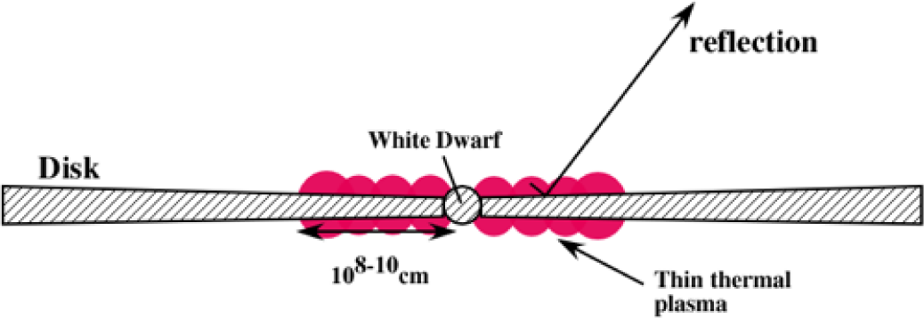
Figure 11: Geometry of the optically thin thermal plasma in outburst. The energy width of the 6.4 keV line, the small contribution from the white dwarf surface to the EW, and $\Omega^{\rm O}/2\pi=0.9^{+0.5}_{-0.4}$ strongly suggest that the plasma is located on the disk like coronae.

This picture is supported also by the Chandra HETG observations (Okada et al., 2008), in which the plasma emission lines are very broad with their Gaussian $\sigma$ as large as $\sim$2000 km s^-1. This is much broader than the thermal velocity, and can be attributed to the plasma being anchored to the disk by, for example, magnetic field and corotating with the disk. A similar disk corona geometry is suggested to explain the X-ray spectrum and the energy width of the emission lines in WZ Sge in outburst (Wheatley & Mauche, 2005).

Note that the absence of the narrow 6.4 keV component can alternatively be understood by invoking the accretion belt (Paczyński, 1978; Kippenhahn & Thomas, 1978) which is an equatorial part of the white dwarf atmosphere being accelerated by the accretion torque and rotating nearly at the local Keplerian velocity ($v_{\rm K}\sin i\sim$4000 km s^-1 in SS Cyg, § 4.1.1). It is suggested from observations that the belt covers significant fraction of the white dwarf surface in outburst (Long et al., 1993; Cheng et al., 1997; Szkody et al., 1998). If so, the 6.4 keV line from the white dwarf should also be broad. Our data of the 6.4 keV line in outburst can be compatible with the existence of the accretion belt.

4.2.2 A possible solution to the large EW of the 6.4 keV line

As explained in § 4.2.1, the width of the 6.4 keV line can be attributed to the Keplerian motion of the disk (and the accretion belt). The observed equivalent width $EW\!=\!208^{+68}_{-27}~{}{\rm eV}$ (table 5), however, can not be explained solely by simple fluorescence due to continuum illumination. Assuming the inclination angle of the disk $i=37^{\circ}$ (Shafter, 1983), the photon index of the incident spectrum $\Gamma=2.3$ (correction is made to the value 2.16 in table 5, see § 4.1.2), the iron abundance of 0.37$Z_{\odot}$, we expect ${\rm EW}\sim 110$ eV at most according to George & Fabian (1991), even if we assume the upper limit of the allowed range of the solid angle $\Omega^{\rm O}/2\pi=1.4$, which may be achieved by taking the accretion belt into account. Since the thickness of matter surrounding SS Cyg is thin, only of order $N_{\rm H}\lesssim 10^{20}$ cm^-2 (§ 4.1.1), there is no other source that can produce 6.4 keV line photons via fluorescence. The large observed equivalent width therefore requires some other mechanism to enhance the intensity around 6.4 keV.

One possible solution is to invoke a Compton shoulder which appears in a lower energy side of a main line due to Compton down scattering. Such a shoulder is resolved with the Chandra HETG in a wide variety of sources such as a HMXB (Watanabe et al., 2003), a ULX (Bianchi et al., 2002), and an AGN (Kaspi et al., 2002). Note that the seed photon of the shoulder in these objects is the 6.4 keV fluorescence line born in Compton-thick clouds, whereas in the current case, we consider the He-like K$\alpha$ line at 6.67 keV, because it is very strong with an equivalent width of 390 eV (table 5). The Compton shoulder of the 6.67 keV line extends down to $\lambda_{0}+2\lambda_{\rm C}$ in wavelength, corresponding to 6.50 keV in energy, in the case of the back scattering, where $\lambda_{0}$ and $\lambda_{\rm C}$ are the wavelength of the 6.67 keV photon and the Compton wavelength (= $h/m_{\rm e}c$), respectively. The low energy end of the shoulder (6.50 keV) is close enough to be merged into the broad 6.4 keV line with a CCD resolution.

In order to evaluate contribution of the 6.67 keV Compton shoulder to the observed EW of the 6.4 keV line, we consider a simple geometrical model, in which a point source of 6.67 keV photons is centered at a height $h$ above a circular slab with a radius of $R_{\rm out}$. We adopt an inclination of the slab to be $i=37^{\circ}$ (Shafter, 1983). Then, the energy of a scattered photon arriving at the observer from any part of the slab can be calculated, because the energy of a scattered photon is uniquely determined by the scattering angle. In calculating the photon energy, we can ignore the Kepler motion of the slab because the situation is in a non-relativistic domain. Assuming that the intrinsic line emission is isotropic, we have calculated the spectrum of the Compton-scattered photons by integrating the emissions from the entire slab. Note that the intensity of the spectrum is affected by the elemental abundance of the slab through probability of the scattering (vs. photoelectric absorption), and absorption of the scattered photons along the path to escape from the slab. We adopt the abundances which we have already measured (§ 3.3). As a result, the cross section of the photoelectric absorption at 6.67 keV is obtained to be $1.15\times 10^{-24}\ {\rm cm^{-2}}$, which is roughly twice as large as that of the Compton scattering. The resultant iron 6.67 keV line spectrum in the case of $h=0.1R_{\rm out}$ is shown in Fig. 12.

Figure 12: Example of the line profile after a single Compton scattering by electrons in the geometrically thin non-relativistic disk. The energy of the source photons is 6.67 keV, which we consider a He-like iron K$\alpha$ line. The inclination angle of the disk is 37^∘. The height of the photon source is $h=0.1R_{\rm out}$ above the disk plane.

The low energy end of the shoulder appears at 6.50 keV as expected, and the high energy end is determined by the edge of the accretion disk.

We have attempted to evaluate the outburst spectra in the 5–9 keV band again by implementing this Compton scattered He-like iron K$\alpha$ line component in the model. In the fitting, the central energies of the iron lines are all fixed at their rest-frame energies (6.97 keV, 6.67 keV, and 6.40 keV). The height of the plasma $h$ is not constrained very well, and hence we also fix it at $0.1R_{\rm out}$, which is expected from the best-fit value of $\Omega^{\rm O}/2\pi=0.9$. The result of the fit is shown in Fig. 13, and its best-fit parameters are summarized in table 6.

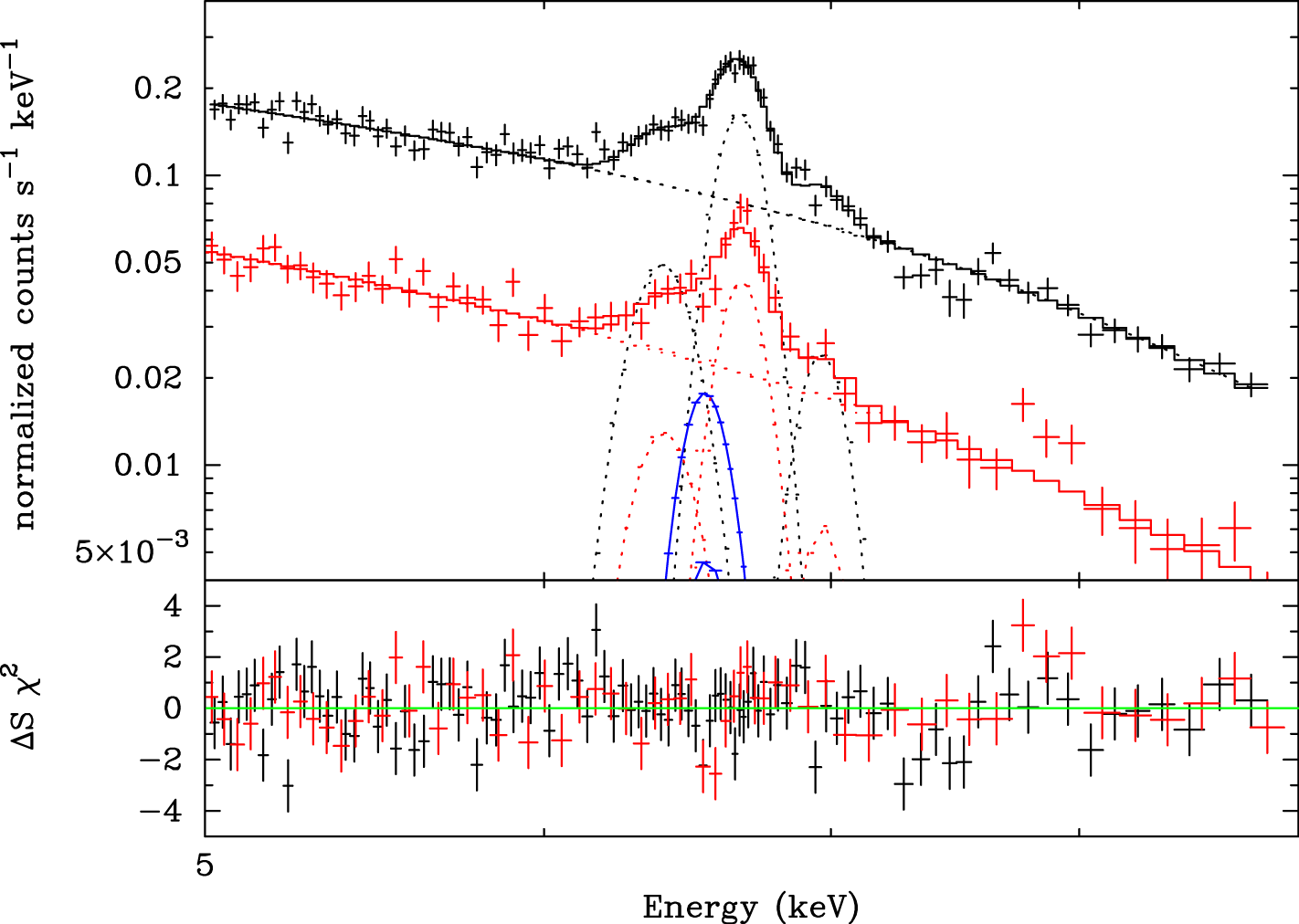
Figure 13: The outburst spectra in the 5–9 keV band with the best-fit model composed of a thermal bremsstrahlung and three iron lines including a Compton shoulder of the He-like K$\alpha$ line in blue color.

Table 6: Best-fit parameters of a thermal bremsstrahlung plus three iron K$\alpha$ lines including a Compton shoulder to the outburst spectra in the 5–9 keV band.

Component	Parameter	Best-fit value
continuum	$kT$ (keV)	$8.0^{+0.6}_{-0.5}$
	normalization	$3.80^{+0.16}_{-0.14}$
H-like line	energy (keV)	6.97 (fixed)
	normalization	$0.81^{+0.18}_{-0.17}$
	EW (eV)	$78^{+17}_{-16}$
He-like line	energy (keV)	6.67 (fixed)
	normalization	$4.93^{+0.25}_{-0.30}$
	EW (eV)	$431^{+22}_{-26}$
Compton	$h/R_{out}$	0.1 (fixed)
	EW (eV)	$42^{+2}_{-3}$
Neutral line	energy (keV)	6.40 (fixed)
	$\sigma$ (keV)	$0.073^{+0.079}_{-0.057}$
	normalization	$1.74^{+0.67}_{-0.41}$
	EW (eV)	$140^{+54}_{-33}$
	$\chi^{2}$(d.o.f)	205.7(157)
	$\chi^{2}_{\nu}$	1.31
In a unit of ($3.02\times 10^{-18}/(4\pi D)^{2}\ EM$), where $EM$ is the emission measure in a unit of ${\rm cm^{-3}}$. In a unit of ($\times 10^{-3}\ {\rm cm^{-2}\ keV^{-1}\ s^{-1}}$) at 1 keV. In units of ($\times 10^{-5}\ {\rm photons\ cm^{-2}\ s^{-1}}$).

Here we have employed a thermal bremsstrahlung as the continuum because it provides a better fit than a power law. The normalization of the Compton shoulder is tied to that of He-like iron K$\alpha$ line according to the expectation from $h=0.1R_{\rm out}$. As a result of the fit, we found that the equivalent width of the broad 6.4 keV line is reduced from $208^{+68}_{-27}$ eV to $140^{+54}_{-33}$ eV. This value is, however, only marginally consistent with the equivalent width predicted from the given reflection scale (${\rm EW}(\Omega/2\pi\!=\!0.9^{+0.5}_{-0.4})\!=\!72^{+40}_{-32}$ eV).

The obtained Gaussian $\sigma$ of the 6.4 keV line, on the other hand, is interpreted to represent the Keplerian velocity of the disk, which is

$$\sqrt{\frac{GM_{WD}}{r}}\;=\;v_{\rm K}(r)\;=\;\left(\frac{\sigma}{E_{0}}\right)\ \frac{c}{\sin i},$$ (4)

where $E_{0}=6.4$ keV is the central energy of the fluorescent iron K$\alpha$ line, $i$ is the inclination angle $\simeq$37^∘. From the Gaussian $\sigma$ evaluated with the Compton shoulder model, $\sigma\!=\!0.073^{+0.079}_{-0.057}$ keV (table 6), we obtain $v_{\rm K}(r)=5700^{+6100}_{-4400}$ km s^-1, resulting in a radius of $r=3.5^{+68.4}_{-2.4}\times 10^{8}$ cm for the 1.19$M_{\odot}$ white dwarf. The optically thin thermal plasma seems to exist on the disk within $r\lesssim 7\times 10^{9}$ cm from the white dwarf. It may be intriguing to compare the spatial extension of the plasma thus obtained with that of an eclipsing dwarf nova in outburst or a nova-like variable. Based on the XMM-Newton observation of the nova-like variable UX UMa, Pratt et al. (2004) measured an elapsed phase for the the hard X-ray eclipse transition to be $\Delta\varphi\leq 0.01$. The binary parameters (Ritter & Kolb (2003) and references therein), on the other hand, indicate an orbital separation of $a=9.7\times 10^{10}$ cm. Hence, the plasma size is estimated to be $\leq 10^{9}$ cm, in good agreement with the current estimation of SS Cyg in outburst.

4.3 Elemental Abundances

The elemental abundances of SS Cyg are summarized in table 3, which are plotted in the left panel of Fig. 14.

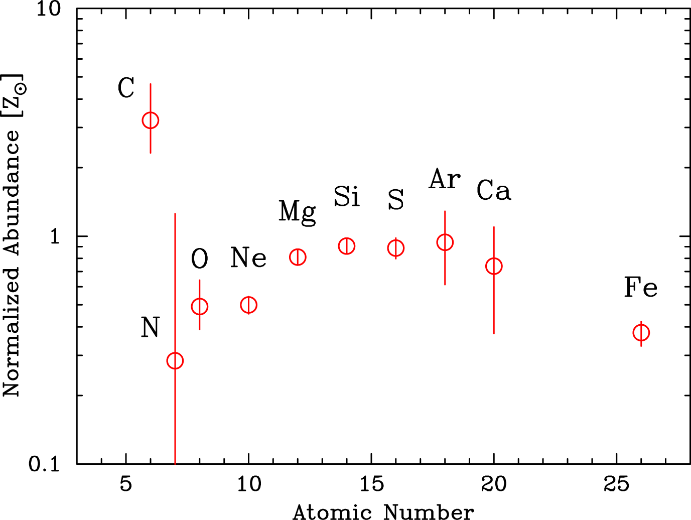
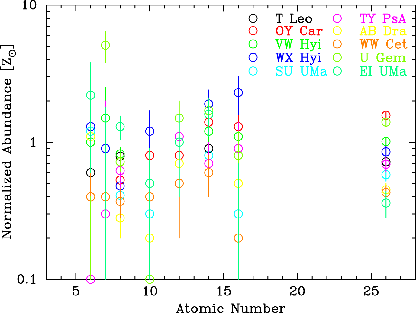
Figure 14: (left) Abundances of SS Cyg obtained with the Suzaku observations (§ 3.3). (right) Abundances of the 10 non-magnetic CVs obtained with the XMM-Newton observations in quiescence (Pandel et al., 2005). Abundances are given relative to the solar values in Anders & Grevesse (1989)

All of the elemental abundances except for C are generally sub-solar. Done & Osborne (1997) determined the abundance of Si, S, and Fe separately, and that of the other elements in common by fitting ASCA outburst spectrum, which are also subsolar. We further resolved the abundances of Mg, Ne, O, N, and C. The right panel of Fig. 14, on the other hand, shows the abundances of 10 non-magnetic CVs obtained with the XMM-Newton observations (Pandel et al., 2005). These abundances are determined also by fits with the same model as ours. Their values are widely distributed from sub-solar to near solar abundances. The abundances of SS Cyg are within these distribution in general.

5 Conclusion

We have presented results of the Suzaku observations on the dwarf nova SS Cyg in quiescence and outburst in 2005 November. The X-ray spectra of SS Cyg are composed of a multi-temperature optically thin thermal plasma model with a maximum temperature of a few tens of keV, its reflection from the white dwarf surface and/or the accretion disk, and a 6.4 keV neutral iron K$\alpha$ line from the reflectors via fluorescence. High sensitivity of the HXD PIN detector and the high spectral resolution of the XIS enable us to disentangle degeneracy between the maximum temperature and the reflection parameters, and to determine the emission parameters with unprecedented precision. The maximum temperature of the plasma in quiescence $kT^{\rm Q}_{\rm max}=20.4^{+4.0}_{-2.6}\,\mbox{(stat.)}\pm 3.0\,\mbox{(sys.)}$ keV is significantly higher than that in outburst $kT^{\rm O}_{\rm max}=6.0^{+0.2}_{-1.3}$ keV. The elemental abundances of the plasma are close to the solar ones for the medium-Z elements (Si, S, Ar) whereas they declines both in lighter and heavier elements. Those of oxygen and iron are 0.46${}^{+0.04}_{-0.03}\,\mbox{(stat.)}\pm 0.01\,\mbox{(sys.)}Z_{\odot}$ and 0.37${}^{+0.01}_{-0.03}\,\mbox{(stat.)}\pm 0.01\,\mbox{(sys.)}Z_{\odot}$. The exception is carbon whose abundance is at least $2Z_{\odot}$ even if we take into account all possible systematic errors. These trends are similar to other dwarf novae observed with XMM-Newton (Pandel et al., 2005).

The solid angle of the reflector subtending over the optically thin thermal plasma is $\Omega^{\rm Q}/2\pi=1.7\pm 0.2\,\mbox{(stat.)}\pm 0.1\,\mbox{(sys.)}$ in quiescence. Since even an infinite slab can subtend a solid angle of $\Omega/2\pi=1$ over a radiation source above it, this large solid angle can be achieved only if the plasma views both the white dwarf and the accretion disk with substantial solid angles. Thanks to high energy resolution of the XIS, we have resolved a 6.4 keV iron K$\alpha$ line into a narrow and broad components (significance of the broad component is $\sim$99%), which also indicate contributions from both the white dwarf and the accretion disk to the reflected continuum spectra. The equivalent widths of them are both $\sim$50 eV. From all these results, we consider the standard optically thin BL formed between the inner edge of the accretion disk and the white dwarf surface (Patterson & Raymond, 1985) as the most plausible model to explain the observed large solid angle. From the equivalent width of the narrow 6.4 keV component, the height of the BL from the white dwarf surface is $h<0.12R_{\rm WD}$. The total equivalent width of the 6.4 keV line ($\sim$100 eV) is consistent with that expected from $\Omega^{\rm Q}/2\pi$, the iron abundance, and the incident illuminating continuum spectrum.

The solid angle of the reflector in outburst $\Omega^{\rm O}/2\pi=0.9^{+0.5}_{-0.4}$, on the other hand, is significantly smaller than that in quiescence, and is consistent with an infinite slab. Since the 6.4 keV iron emission line is broad with no narrow component ($\lesssim$20% of the broad component), the reflection originates from the accretion disk. The accretion belt can also contribute to the reflection. The 6.4 keV line from the accretion belt is expected to be broad, which is consistent with the absence of the narrow 6.4 keV component. The EW of the 6.4 keV line is so large that it cannot be interpreted within a simple scheme of reflection from the disk. Even if Compton down-scattering of the observed He-like K$\alpha$ line is taken into account, we can only find a solution which marginally reconciles the large EW with the solid angle of the reflector. We consider the optically thin thermal plasma in outburst as being distributed on the accretion disk. The Chandra HETG observation in outburst revealed that the He-like and H-like emission lines from O, Ne, Mg, and Si are broad and their widths ($\sim$2000 km s^-1) are consistent with those expected from the Keplerian velocity of the accretion disk (Okada et al., 2008). This fact suggests that the optically thin thermal plasma is anchored to the accretion disk and the accretion belt by magnetic field, for example, like solar coronae.

Appendix A Low energy response of XIS1

In order to analyze spectra with XIS1 in the energy band $\lesssim$0.5 keV where the energy response is affected by accumulation of contaminating material, we have checked the energy response of the XIS-1 with the PKS2155–304 data taken between 2005 November 30 and 2005 December 1 (seq.#700012010), which were taken close enough to our SS Cyg observations. Although the observation is originally planned to continue for a 60 ks effective exposure time, part of the observation suffered a light-leak accident and the CCD chip is irradiated by optical and UV photons. After removing these time intervals, 39.4 ks data remain in total. We then created the same on-source and background regions as those adopted in the SS Cyg observations, and created the response file of XIS1. The default correction was made for the contamination.

Between 0.1 and 10 keV, PKS2155$-$304 has been well represented by a curved spectrum with an energy slope gradually steepening from 1.1 to 1.6 (Giommi et al., 1998). We therefore fit our XIS1 spectrum with a broken power-law model

$$F(E) = K(E/1~{}{\rm keV})^{-\Gamma_{1}}\qquad\qquad\quad(for~{}~{}E\leq E_{c})$$ (5)

$$= KE_{c}^{\Gamma_{2}-\Gamma_{1}}\times(E/1~{}{\rm keV})^{-\Gamma_{2}}~{}~{}(for~{}~{}E\geq E_{c}),$$ (6)

where $\Gamma_{1}$ and $\Gamma_{2}$ are power law photon indexes, $K$ is normalization factor, $E_{c}$ is a break energy, and see if the low energy calibration is enough for our analysis. The hydrogen column density to PKS2155 is $16.9\times 10^{19}~{}{{\rm cm^{-2}}}$ from past infrared observations. The result of fit is shown in the left panel of Fig. 15.

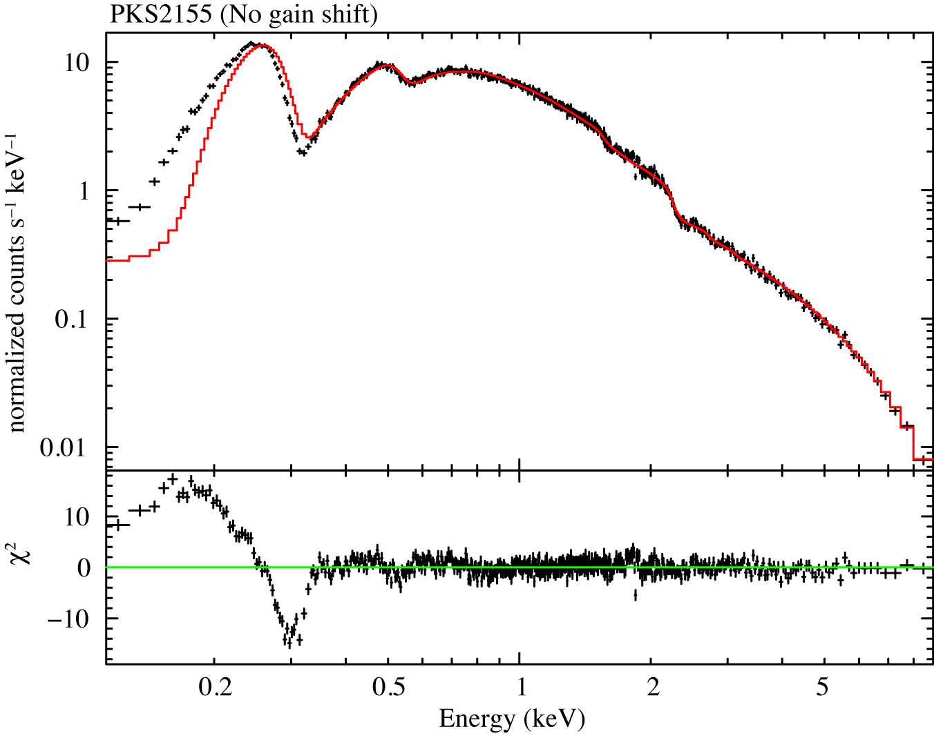
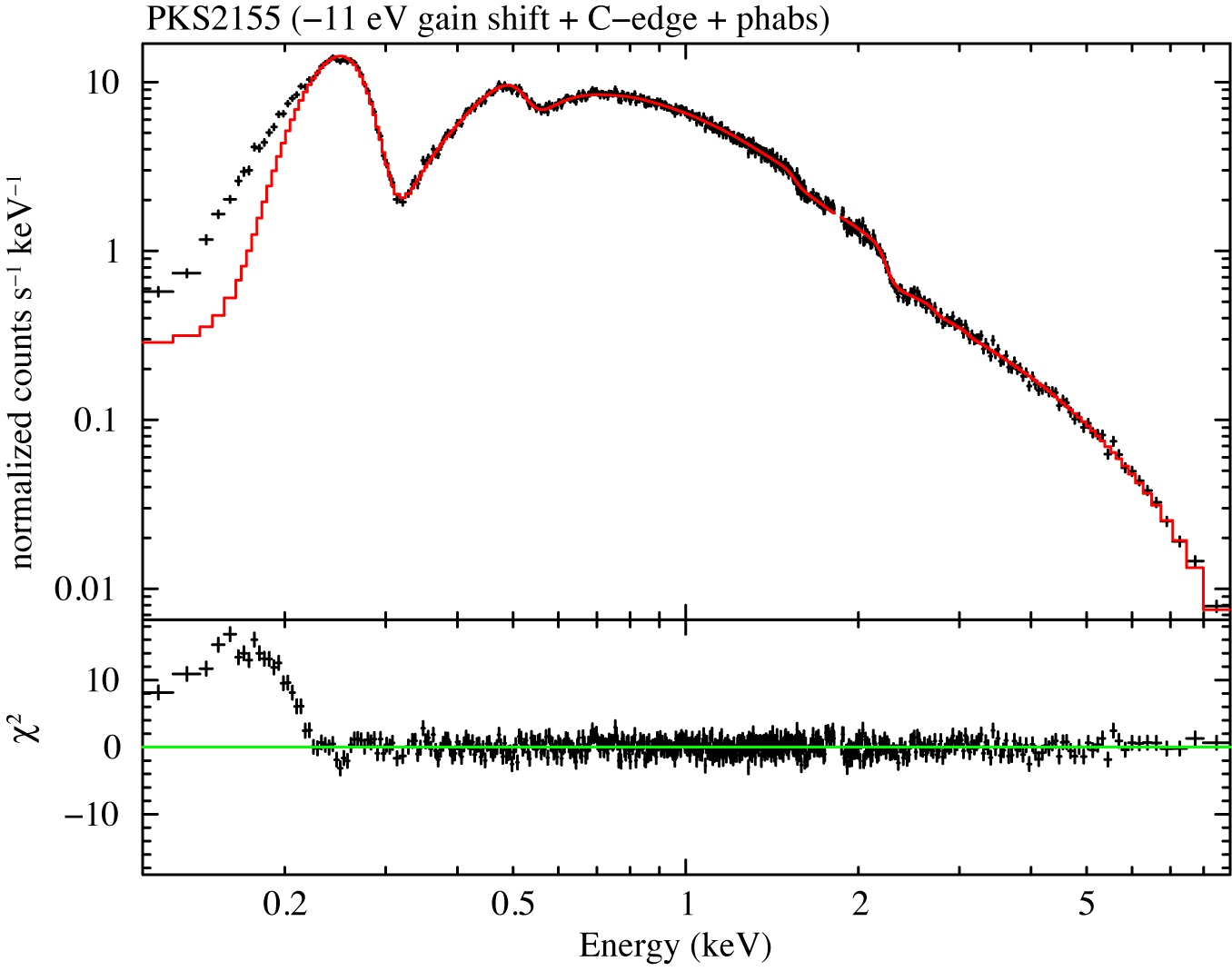
Figure 15: Spectral fitting of XIS-1 in the energy range of 0.1–10 keV before adjusting the energy scale (left), and after adjusting the gain and applying additional absorption. After these treatments, the energy band above 0.226 keV can safely be used for spectral analysis.

The fit below $\sim$0.35 keV is not very well, and there is evidence of gain shift between 0.5–0.6 keV. Hence we apply an energy offset to the model by 1 eV step, and found that the $-$11 eV shift gives the smallest reduced $\chi^{2}$ value. The remaining residuals are adjusted by introducing additional hydrogen column density and a carbon K edge at 0.2842 keV, which are both deemed associated with the contaminant of the XIS. The result of the fit is shown in the right panel of Fig. 15 and its best-fit parameters are summarized in table 7.

Table 7: Best-fit parameters of additional absorption component to fit the spectrum of PKS2155$-$304.

Model	parameter
Gain offset (eV)	$-$11 (fixed)
$\tau$ of carbon K edge	$0.88\pm 0.05$
$N_{\rm H}$ ($10^{19}$ cm-2)	$8.2\pm 0.7$
$\chi^{2}$ (d.o.f.)	640 (547)

The additional photoelectric absorption and the edge significantly improves the fit in 0.3–0.5 keV, and the spectrum down to 0.226 keV can be well represented by the broken power-law model. In the analysis of the Suzaku SS Cyg data, we always apply additional absorption column density of $N_{\rm H}=8.2\times 10^{19}$ cm^-2 and the carbon edge with an optical depth of $\tau=0.88$ at 0.2842 keV. The amount of gain offset is different from observation to observation. We have checked the offsets during the Suzaku observations of SS Cyg in quiescence and outburst in the same way as is described above to find that no offset ($\lesssim 2$ eV) is required for both observations.

References

- Anders & Grevesse (1989) Anders, E., & Grevesse, N. 1989, Geochim. Cosmochim. Acta, 53, 197
- Arnaud (1996) Arnaud, K. A. 1996, Astronomical Data Analysis Software and Systems V, 101, 17
- Baskill et al. (2005) Baskill, D. S., Wheatley, P. J., & Osborne, J. P. 2005, MNRAS, 357, 626
- Bath & Pringle (1982) Bath, G. T., & Pringle, J. E. 1982, MNRAS, 199, 267
- Bianchi et al. (2002) Bianchi, S., Matt, G., Fiore, F., Fabian, A. C., Iwasawa, K., & Nicastro, F. 2002, A&A, 396, 793
- Boldt (1987) Boldt, E. 1987, Phys. Rep., 146, 215
- Cannizzo (1993) Cannizzo, J. K. 1993, ApJ, 419, 318
- Cheng et al. (1997) Cheng, F. H., Sion, E. M., Horne, K., Hubeny, I., Huang, M., & Vrtilek, S. D. 1997, AJ, 114, 1165
- Cordova et al. (1984) Cordova, F. A., Chester, T. J., Mason, K. O., Kahn, S. M., & Garmire, G. P. 1984, ApJ, 278, 739
- Cordova et al. (1980) Cordova, F. A., Chester, T. J., Tuohy, I. R., & Garmire, G. P. 1980, ApJ, 235, 163
- Done & Osborne (1997) Done, C., & Osborne, J. P. 1997, MNRAS, 288, 649
- Friend et al. (1990) Friend, M. T., Martin, J. S., Connon-Smith, R., & Jones, D. H. P. 1990, MNRAS, 246, 654
- Gehrels & Williams (1993) Gehrels, N., & Williams, E. D. 1993, ApJ, 418, L25
- George & Fabian (1991) George, I. M., & Fabian, A. C. 1991, MNRAS, 249, 352
- Giommi et al. (1998) Giommi, P., et al. 1998, A&A, 333, L5
- Harrison et al. (1999) Harrison, T. E., McNamara, B. J., Szkody, P., McArthur, B. E., Benedict, G. F., Klemola, A. R., & Gilliland, R. L. 1999, ApJ, 515, L93
- Hoare & Drew (1991) Hoare, M. G., & Drew, J. E. 1991, MNRAS, 249, 452
- Huang et al. (1996) Huang, M., Sion, E. M., Hubeny, I., Cheng, F. H., & Szkody, P. 1996, ApJ, 458, 355
- Ishida et al. (2007) Ishida, M., Okada, S., Nakamura, R., Terada, Y., Hayashi, T., Mukai, K., & Hamaguchi, K. 2007, Progress of Theoretical Physics Supplement, 169, 178
- Jones & Watson (1992) Jones, M. H., & Watson, M. G. 1992, MNRAS, 257, 633
- Kaastra et al. (1996) Kaastra, J. S., Mewe, R., & Nieuwenhuijzen, H. 1996, UV and X-ray Spectroscopy of Astrophysical and Laboratory Plasmas : Proceedings of the Eleventh Colloquium on UV and X-ray … held on May 29-June 2, 1995, Nagoya, Japan. Edited by K. Yamashita and T. Watanabe. Tokyo : Universal Academy Press, 1996. (Frontiers science series ; no. 15)., p.411, 411
- Kaspi et al. (2002) Kaspi, S., et al. 2002, ApJ, 574, 643
- Kippenhahn & Thomas (1978) Kippenhahn, R., & Thomas, H.-C. 1978, A&A, 63, 265
- Kokubun et al. (2007) Kokubun, M., et al. 2007, PASJ, 59, 53
- Koyama et al. (2007) Koyama, K., et al. 2007, PASJ, 59, 23
- Liedahl et al. (1995) Liedahl, D. A., Osterheld, A. L., & Goldstein, W. H. 1995, ApJ, 438, L115
- Long et al. (1993) Long, K. S., Blair, W. P., Bowers, C. W., Davidsen, A. F., Kriss, G. A., Sion, E. M., & Hubeny, I. 1993, ApJ, 405, 327
- Magdziarz & Zdziarski (1995) Magdziarz, P., & Zdziarski, A. A. 1995, MNRAS, 273, 837
- Makishima (1986) Makishima, K. 1986, The Physics of Accretion onto Compact Objects, 266, 249
- Marsh & Horne (1998) Marsh, T. R., & Horne, K. 1998, MNRAS, 299, 921
- Mauche (2004) Mauche, C. W. 2004, ApJ, 610, 422
- Mauche & Robinson (2001) Mauche, C. W., & Robinson, E. L. 2001, ApJ, 562, 508
- Mauche et al. (1995) Mauche, C. W., Raymond, J. C., & Mattei, J. A. 1995, ApJ, 446, 842
- Mauche et al. (1991) Mauche, C. W., Wade, R. A., Polidan, R. S., van der Woerd, H., & Paerels, F. B. S. 1991, ApJ, 372, 659
- Mewe et al. (1986) Mewe, R., Lemen, J. R., & van den Oord, G. H. J. 1986, A&AS, 65, 511
- Mewe et al. (1985) Mewe, R., Gronenschild, E. H. B. M., & van den Oord, G. H. J. 1985, A&AS, 62, 197
- Meyer & Meyer-Hofmeister (1981) Meyer, F., & Meyer-Hofmeister, E. 1981, A&A, 104, L10
- Mitsuda et al. (2007) Mitsuda, K., et al. 2007, PASJ, 59, 1
- Mukai et al. (1997) Mukai, K., Wood, J. H., Naylor, T., Schlegel, E. M., & Swank, J. H. 1997, ApJ, 475, 812
- Okada et al. (2008) Okada, S., Nakamura, R., & Ishida, M. 2008, ApJ, 680, 695
- Osaki (1996) Osaki, Y. 1996, PASP, 108, 39
- Osaki (1974) Osaki, Y. 1974, PASJ, 26, 429
- Paczyński (1978) Paczyński, B. 1978, Nonstationary Evolution of Close Binaries, 89
- Pandel et al. (2005) Pandel, D., Córdova, F. A., Mason, K. O., & Priedhorsky, W. C. 2005, ApJ, 626, 396
- Patterson et al. (1998) Patterson, J., Richman, H., Kemp, J., & Mukai, K. 1998, PASP, 110, 403
- Patterson & Raymond (1985) Patterson, J., & Raymond, J. C. 1985, ApJ, 292, 535
- Pratt et al. (2004) Pratt, G. W., Mukai, K., Hassall, B. J. M., Naylor, T., & Wood, J. H. 2004, MNRAS, 348, L49
- Pringle & Savonije (1979) Pringle, J. E., & Savonije, G. J. 1979, MNRAS, 187, 777
- Pringle (1977) Pringle, J. E. 1977, MNRAS, 178, 195
- Ricketts et al. (1979) Ricketts, M. J., King, A. R., & Raine, D. J. 1979, MNRAS, 186, 233
- Ritter & Kolb (2003) Ritter, H., & Kolb, U. 2003, A&A, 404, 301
- Robinson et al. (1978) Robinson, E. L., Nather, R. E., & Patterson, J. 1978, ApJ, 219, 168
- Schoembs (1986) Schoembs, R. 1986, A&A, 158, 233
- Serlemitsos et al. (2007) Serlemitsos, P. J., et al. 2007, PASJ, 59, 9
- Smak (1984) Smak, J. 1984, PASP, 96, 5
- Shafter (1983) Shafter, A. W. 1983, Ph.D. Thesis,
- Shakura & Syunyaev (1973) Shakura, N. I., & Syunyaev, R. A. 1973, A&A, 24, 337
- Sion et al. (1996) Sion, E. M., Cheng, F.-H., Huang, M., Hubeny, I., & Szkody, P. 1996, ApJ, 471, L41
- Szkody et al. (1998) Szkody, P., Hoard, D. W., Sion, E. M., Howell, S. B., Cheng, F. H., & Sparks, W. M. 1998, ApJ, 497, 928
- Takahashi et al. (2007) Takahashi, T., et al. 2007, PASJ, 59, 35
- Tylenda (1977) Tylenda, R. 1977, Acta Astronomica, 27, 235
- Warner & Woudt (2002) Warner, B., & Woudt, P. A. 2002, MNRAS, 335, 84
- Warner (1995) Warner, B. 1995, Cambridge Astrophysics Series, 28, pp.28
- Watanabe et al. (2003) Watanabe, S., et al. 2003, ApJ, 597, L37
- Wheatley & Mauche (2005) Wheatley, P. J., & Mauche, C. W. 2005, The Astrophysics of Cataclysmic Variables and Related Objects , 330, 257
- Wheatley et al. (2003) Wheatley, P. J., Mauche, C. W., & Mattei, J. A. 2003, MNRAS, 345, 49