Phase statistics of seismic coda waves

Abstract

We report the analysis of the statistics of the phase fluctuations in the coda of earthquakes recorded during a temporary experiment deployed at Pinyon Flats Observatory, California. The observed distributions of the first, second and third derivatives of the phase in the seismic coda exhibit universal power-law decays whose exponents agree accurately with circular Gaussian statistics. The correlation function of the spatial phase derivative is measured and used to estimate the mean free path of Rayleigh waves.

In the short-period band ($>1$ Hz) , ballistic arrivals of seismic waves are often masked by scattered waves due to small-scale heterogeneities in the lithosphere. The scattered elastic waves form the pronounced tail of seismograms known as the seismic coda (Aki, 1969; Aki and Chouet, 1975). Even when scattering is prominent, it is still possible to define the phase of the seismic record by introducing the complex analytic signal $\psi(t,\mathbf{r})=A(t,\mathbf{r})e^{\mathrm{i}\phi(t,\mathbf{r})}$, with $A$ the amplitude and $\phi$ the phase. In the past, many studies have focused on the modeling of the mean field intensity $I(t)=\langle A(t)^{2}\rangle$ (see Sato and Fehler, 1998, for review). The goal of the present paper is to study the statistics of the phase field in the coda. In the coda, the measured displacements result from the superposition of many partial waves which have propagated along different paths between the source and the receiver. Each path consists of a sequence of scattering events that affect the phase of the corresponding partial wave in a random way. For narrow-band signals, the phase field can therefore be written as $\phi(t,\mathbf{r})=\omega t+\delta\phi(t,\mathbf{r})$, where $\omega$ is the central frequency, and $\delta\phi$ denotes the random fluctuations. The trivial cyclic phase $\omega t$ cancels when a spatial phase difference is considered between two neighbouring points. Spatially resolved measurements are facilitated by dense arrays of seismometers that have been set up occasionally. We note that the phase of coda waves has not been given much attention so far. The advantage of phase is that it is not affected by the earthquake magnitude, and that it contains pure information on scattering, not blurred by absorption effects. For the statistical analysis of amplitude and phase fluctuations of direct arrivals, we refer the reader to e.g. Zheng and Wu (2005).

I Phase distributions

We study data sets from a temporary experiment deployed at Pinyon Flat Observatory (PFO), California, in 1990 by an IRIS program. This site exhibits a high level of regional seismic activity. The array (see Fig. 1) contained 58 3-components L-22 sensors (2Hz) and was configured as a grid and two orthogonal arms with sensor spacings of 7 meters within the grid and 21 meters on the arms (Owens et al., 1991). We selected 8 earthquakes of magnitude greater than 2 with good signal to noise ratio in the coda. Typically, epicentral distances are less than 110 km and the coda lasts more than 30 seconds after the direct arrivals.

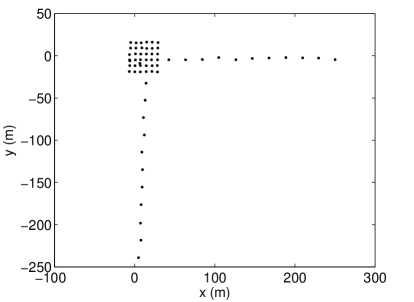
Figure 1: Geometry of the seismic array

To perform the statistical analysis, we filtered the signal in a narrow frequency band centered around 7 Hz ($\pm 5\%$) and selected a 15 s time window starting around 5 seconds after the direct arrivals. In this time window, the signal is believed to be dominated by multiple scattering and is highly coherent along the array (Margerin et al., 2008). We evaluate the Hilbert transform of the vertical displacement which yields the imaginary part of the complex analytic signal $\psi(t,\mathbf{r})=A(t,\mathbf{r})e^{i\phi(t,\mathbf{r})}$. From the complex field, two definitions of the phase can be given: (1) The wrapped phase $\phi$ is defined as the argument of the complex field $\psi$ in the range $\left(-\pi:\pi\right]$. (2) The unwrapped phase $\phi_{u}$ is obtained by correcting for the $2\pi$ jumps – occurring when $\phi$ goes through the value $\pm\pi$ - to obtain a continuous function with values in $\mathbb{R}$. The $\phi$ distribution is flat (SOL, ). However, more information can be extracted by considering higher-order statistics of the phase. For this purpose we consider the spatial derivative of the phase, which can be estimated in two different ways.

(1) The first measurement relies on the difference of the wrapped phases $\Delta\phi$ between two seismometers separate by a distance $\delta$. Applying the simple finite difference formula $\phi^{\prime}\approx\Delta\phi/\delta$ an estimate of the spatial derivative is obtained. Note that the phase difference $\Delta\phi$ takes values between $-2\pi$ and $+2\pi$ which does not allow a precise estimate for the distribution of the derivative for values roughly larger than $\pi/\delta$. Beyond this value our measurements will be dominated by finite difference artifacts and the distribution is biased by the $2\pi$ jumps occurring within the distance $\delta$.

(2) The second method uses the difference of the phases $\phi_{u}$ spatially unwrapped at each time step. This yields another estimate of the derivative: $\phi^{\prime}\approx\Delta\phi_{u}/\delta$ which is expected to suppress finite difference artifact. In practice it is impossible to discriminate a rare but physical large phase jump from a small fluctuation that causes a $2\pi$ jump just within the range $\delta$. The only possibility along 1-D arrays is to impose that the largest admissible phase difference between two stations be smaller than $\pi$. Hence this $\phi^{\prime}$ estimate takes values in $(-\pi/\delta:\pi/\delta]$ and is biased close to $\pi/\delta$ by the unwrapping processing errors. In the limit $\delta\to 0$, the two definitions ought to be equivalent because the probability of phase jumps between the two stations tends to 0. By averaging over the 8 seismic records, the lag-time in the coda, the east-west and north-south orientations, and the sensor positions within the array’s grid at fixed $\delta=7$m, we calculate the two resulting phase derivative distributions which are shown to be non-uniform in Figure 2. It is also instructive to consider the second (third) derivatives of the phase which are governed by the 3 (4)-point statistics which are plotted in Figure 3. Higher-order derivatives are obtained by applying standard finite difference formulas to the wrapped phase (this choice is explained in the next section). Since the three first derivative distributions are even functions, we only represent the positive values. They have all similar properties. For small values of the random variables, the distributions are nearly flat. For larger values, the distributions are governed by a power-law decay except for some peaks which stem from the finite distance between the seismic stations. In the following section, we will demonstrate that the transition between the two behaviours is governed by the wavelength and that the power-law decay is a very accurate signature of the Gaussian nature of the vertical displacements.

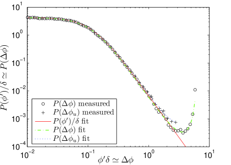
Figure 2: Distribution of the first derivative of the phase normalized by the inter-station distance $\delta$ and measured using finite difference formula. ($\circ$): wrapped phase; ($+$): unwrapped phase. The colour lines represent the fits with Gaussian theory. Green: wrapped phase; blue: unwrapped phase; red : phase derivative. The fitting parameters are $Q=2.774\ 10^{-4}\ m^{-2}$ and $g(\delta)=0.993204$.

Seismic coda is believed to be composed of multiply scattered waves. Upon scattering, the many partial waves - associated with different paths in the medium - would achieve random and independent phase shifts. The Gaussian nature would then follow from the central limit theorem. We will thus assert that the coda waves obey circular Gaussian statistics (CGS) according to which the joint probability of N complex field displacements $\psi_{i}$, recorded at positions $r_{i}$, is written as

$$P(\psi_{1}\cdots\psi_{N})=\frac{1}{\pi^{N}\det\textbf{C}}\exp\left[-\sum_{i,j}^{N}\psi_{i}^{*}\textbf{C}_{ij}^{-1}\psi_{j}\right],$$ (1)

where $\textbf{C}_{ij}=\langle\psi_{i}\psi_{j}^{*}\rangle$ is the covariance matrix (Goodman, 1985). It is convenient to use normalized fields so that $\textbf{C}_{ii}=1$. Then, the off-diagonal elements are equal to the field correlation function $\textbf{C}_{ij}=C(\mid r_{i}-r_{j}\mid)$. From the joint distribution of two fields, the probability distribution of the phase difference at two points located $\delta$ apart can be obtained by integrating over the amplitudes (Cowan et al., 2007):

$$P(\Delta\phi)=\tilde{P}\left[\frac{1-g^{2}}{1-F^{2}}\right]\left[1+\frac{F\cos^{-1}\left(-F\right)}{\sqrt{1-F^{2}}}\right]$$ (2)

where $F=g\cos(\Delta\phi)$ and $g=\left<\psi(r-\delta/2)\psi*(r+\delta/2)\right>$; $\tilde{P}=(2\pi-|\Delta\phi|)/4\pi^{2}$ if $\Delta\phi$ is the difference of the wrapped phase and $\tilde{P}=1/{2\pi}$ if $\Delta\phi$ is the difference of the unwrapped phase $\Delta\phi_{u}$. In the limit $\delta\to\infty$ of totally uncorrelated fields $P(\Delta\phi)=\tilde{P}$. In the limit $\delta\to 0$, we get the following formula for the phase derivative Genack et al. (1999):

$$P(\phi^{\prime})=\frac{1}{2}\frac{Q}{\left[Q+\phi^{\prime 2}\right]^{3/2}}.$$ (3)

where $Q=-C^{\prime\prime}(0)=2(1-g)/\delta^{2}$ for $\delta\to 0$. Figure 2 demonstrates that the phase difference between two nearby seismometers follows the prediction of Gaussian circular statistics with excellent accuracy: we observe a good agreement between the theoretical distribution of $\phi^{\prime}$ (Eq. 3) and the measurements over 3 orders of magnitude in probability and 2 orders of magnitude in derivative. A clear discrepancy occurs for large values - typically when $\phi^{\prime}\approx\pi/\delta$ - which can be perfectly explained by the finite distance between the seismic stations. This is demonstrated in the same plot which shows excellent agreement between formula (2) and the measured finite-difference statistics of the phase. We observe that the formula for the derivative (3) agrees with the observations on a larger range when the estimate of $\phi^{\prime}$ is based on the wrapped phase difference. As a consequence, we prefer this method to find the higher derivatives.

In the frequency band of interest, there is experimental evidence that the vertical component of the coda is dominated by scattered Rayleigh surface waves (Margerin et al., 2008). As a consequence, we expect the correlation function of the field to be given by (Aki, 1957)

$$C(r)=\langle\psi(0)\psi^{*}(r)\rangle=\mathrm{J_{0}}(kr)\exp(-r/2\ell),$$ (4)

which agrees well with observations (SOL, ). Equation 4 contains two length scales: the wavelength $2\pi/k$ and the scattering mean free path $\ell$. We emphasize that formula (4) is valid even when the medium is slightly inelastic. Weak absorption does not enter the correlation function obtained from the long-time-tail of a diffuse wavefield (van Tiggelen et al., 2006). The form of the correlation function (4) implies that $Q\simeq k^{2}/2$, if $k\ell\gg 1$. Using the parameter $Q$ obtained by fitting the data with equation (3), we infer a dominant wavelength $\lambda$ of the order of $267$ m which agrees with the one predicted on the basis of the vertical profile of the elastic constants below the PFO array (Vernon et al., 1998). $Q$ offers an accurate way of estimating the wavelength, alternative to SPAC measurements (Aki, 1957). The use of a narrow band signal is crucial because the parameters $g$ and $Q$ strongly depend on frequency.

From the joint Gaussian distribution of 3 and 4 fields, we can derive analytically the joint probability functions $P(\phi^{\prime},\phi^{\prime\prime}),$ $P(\phi^{\prime},\phi^{\prime\prime},\phi^{\prime\prime\prime})$ , featuring two new constants $R$ and $S$ (Cowan et al., 2007). From these formulas, the marginal distributions $P(\phi^{\prime\prime})$, $P(\phi^{\prime\prime\prime})$ can be evaluated numerically. The probability distributions of the first, second, and third derivatives of the phase exhibit an asymptotic power-law decay with exponents $-3$, $-2$, $-5/3$, respectively. These universal exponents (i.e. independent of the medium properties) can be obtained analytically and provide a sensitive fit-independent test of the Gaussian nature of the seismic coda. This is illustrated in Figure 3. The agreement leaves no doubt that coda waves are in the multiple scattering regime.

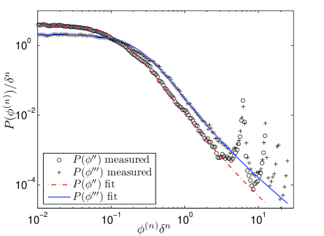
Figure 3: Comparison of the Gaussian theory and observations for the phase derivatives distribution $P(\phi^{(n)})$ where $n=1$ or $2$ denotes the $n^{th}$ derivative of $\phi$ with respect to the spatial coordinate. From the fit we find: $Q=2.774\ 10^{-4}\ m^{-2}$, $R=2.75\ 10^{-2}\ m^{-2}$ and $S=4.0\ 10^{-2}\ m^{-2}$.

II Phase Difference Correlations

We have shown that the distributions of the phase derivatives provide accurate information on the short-range correlation properties of the field. In the following we use the phase difference correlations to put some constraints on the degree of heterogeneity which is responsible for long-range correlations along the array. For Gaussian statistics and for surface waves obeying Eq. (4), the phase derivative correlation function is (van Tiggelen et al., 2006):

$$C_{\phi^{\prime}}(r)\equiv\left<\phi^{\prime}(0)\phi^{\prime}(r)\right>=({k}/{\pi r})\exp(-r/\ell)$$ (5)

for $r>\lambda$. Formula (5) has one crucial property. Contrary to the field correlation function $C$, $C_{\phi^{\prime}}$ does not oscillate on the wavelength scale but decreases with the mean free path as the sole characteristic length scale. Any determination of the mean free path based on formula (4) is impossible because the exponential decay is masked by the rapid cyclic oscillations.

As above, we estimate the phase derivative correlation function in a finite difference approximation using the formula $C_{\phi^{\prime}}(r)\simeq\langle(\Delta\phi_{u}(r^{\prime})\Delta\phi_{u}(r^{\prime\prime})\rangle/\delta^{2}=C_{\Delta\phi_{u}}(|r^{\prime}-r^{\prime\prime}|)/\delta^{2}$. Contrary to the probability distribution, we found out that the unwrapped phase difference offers a better estimate for the phase derivative. The wrapped phase difference correlation function is too much dominated by large $2\pi$ jumps with no physical interest.

The unwrapped phase difference correlation $C_{\Delta\phi_{u}}(r)$ is measured along the two orthogonal arms with an aperture of $252$ m and $\delta=21$ m interstation distance. The data are averaged over orientation, lag-time in the coda and seismic events. The result is presented in linear scale in the main part of Figure 4 and shows a decay dominated by the $1/r$ factor along the arms of the array, as predicted by formula (5). This supports our 2D picture of wave diffusion. Due to the finite difference $C_{\phi^{\prime}}(r=0)$ achieves a finite value at $r=0$, which we found to be consistent with the variance of the unwrapped phase difference calculated from $\langle\Delta\phi_{u}^{2}\rangle=\int_{-\pi}^{\pi}d\Delta\phi_{u}\,(\Delta\phi_{u})^{2}P(\Delta\phi_{u})$ and $g(\delta)=0.98$. The parameter $g(\delta)$ has been determined independently by fitting the observed distribution of $P(\Delta\phi_{u})$ with formula (2) for $\delta=21$ m.

Different reasons exist why it is more difficult to measure the correlation function of the phase derivative than e.g. the probability distributions. First, 4th-order statistics require more averaging to suppress unwanted fluctuations in the data. Secondly, the interstation distance $\delta=21$ m along the arms reduces the correlation between the fields at two nearby stations significantly, which favours systematic errors in the derivative. Finally, due to frequent breakdowns of the sensors located near the ends of the arms, the data could not be averaged over all sensor positions and all seismic events. As a consequence the correlations for distances $r>180$ m had to be excluded.

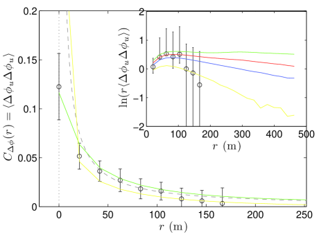
Figure 4: Unwrapped phase difference correlation function. ($\circ$): experimental results. Dashed line: $1/r$ fit. Inset: logarithm of the correlation multiplied by $r$ for data ($\circ$ with error bars) and numerical simulations at fixed $k$ and $\ell=10$ km (green), $\ell=1$ km (red), $\ell=500$ m (red) and $\ell=200$ m (yellow).

Since formula 5 is valid only in the limit $\delta\to 0$, we have evaluated the impact of the finite inter-station distance inherent to our experimental set-up. To this end, we have simulated N correlated Gaussian random field displacements on a virtual array with the PFO geometry. The results for different values of $\ell$ at fixed $k$ are shown in Figure 4 together with the experimental results. The simulated function $\log(r\times C_{\Delta\phi_{u}})$ exhibits a linear decay with a slope $-1/\ell$ as was seen for $\delta\to 0$ in Eq. (5) (see inset in Figure 4). Therefore, correlations of finite-size phase difference still offer direct access to the mean free path of the waves in the crust. It is quite encouraging to see (inset Figure 4) that the asymptotic exponential regime is already reached for $r>\lambda/5$. We find that the $-1/\ell$ slope could in principle be measured if the aperture of the network would have been a few wavelengths in size ($>500$ m), which in general is much smaller than the mean free path. Unfortunately, the experimental error bars of our data set are too large to permit accurate estimates of $\ell$ at PFO although it can roughly be bounded between 1 km and 10 km, much smaller than the typical path (40 km) taken by coda waves coda during 20 s. This has to be interpreted as a rough estimate for the mean free path of the Rayleigh waves.

In conclusion, from their observed first three spatial derivatives of phase, seismic coda waves are proved to obey Gaussian statistics with high accuracy, with a local correlation on the scale of the wavelength. At longer scales, we demonstrate that the correlation function of the spatial derivative of phase offers a new, promising opportunity to measure directly the mean free path $\ell$ of seismic waves. This measure is not affected by absorption neither to scattering anisotropy. As opposed to the coherent backscattering effect (Larose et al., 2004), the proposed method does not require the sensors to be located in the near field of the source, but requires an array of seismic stations with sub-wavelength spacing between stations and with a total aperture of a few wavelengths. Our work highlights the phase as a useful physical object to study seismic coda waves.

We thank J. Page, M. Campillo, P. Roux and E. Larose for useful discussions.

References

- Aki (1969) K. Aki, J. Geophys. Res. 74, 615 (1969).
- Aki and Chouet (1975) K. Aki and B. Chouet, J. Geophys. Res. 80, 3322 (1975).
- Sato and Fehler (1998) H. Sato and M. Fehler, Seismic wave propagation and scattering in the heterogeneous Earth (AIP Press/Springer Verlag, New York, 1998).
- Zheng and Wu (2005) Y. Zheng and R.-S. Wu, Geophys. Res. Lett. 32, 14314 (2005).
- Owens et al. (1991) T. J. Owens, P. N. Owens, P. N. Anderson, and D. E. McNamara, Tech. Rep., Incorporated Research Institution in Seismology (1991).
- Margerin et al. (2008) L. Margerin, M. Campillo, B. Van Tiggelen, and R. Hennino, ArXiv e-prints 803 (2008), eprint 0803.1114.
- (7) See epaps document no. [ ] for formulae. this document can be reached through a direct link in the online article’s html reference section or via the epaps homepage (http://www.aip.org/pubservs/epaps.html).
- Goodman (1985) J. W. Goodman, Statistical optics (New York: Wiley, 1985, 1985).
- Cowan et al. (2007) M. L. Cowan, D. Anache-Ménier, W. K. Hildebrand, J. H. Page, and B. A. van Tiggelen, Phys. Rev. Lett. 99, 094301 (2007).
- Genack et al. (1999) A. Z. Genack, P. Sebbah, M. Stoytchev, and B. A. van Tiggelen, Phys. Rev. Lett. 82, 715 (1999).
- Aki (1957) K. Aki, Bull. Earthq. Res. Inst. 35, 415 (1957).
- van Tiggelen et al. (2006) B. A. van Tiggelen, D. Anache, and A. Ghysels, Europhysics Letters 74, 999 (2006).
- Vernon et al. (1998) F. L. Vernon, G. L. Pavlis, T. J. Owens, D. E. Macnamara, and P. N. Anderson, Bull. Seism. Soc. Am. 88, 1548 (1998).
- Larose et al. (2004) E. Larose, L. Margerin, B. A. van Tiggelen, and M. Campillo, Phys. Rev. Lett. 93, 048501 (2004).