Aspects of quantum phase transitions

Abstract

A unified description of i) classical phase transitions and their remnants in finite systems and ii) quantum phase transitions is presented. The ensuing discussion relies on the interplay between, on the one hand, the thermodynamic concepts of temperature and specific heat and on the other, the quantal ones of coupling strengths in the Hamiltonian. Our considerations are illustrated in an exactly solvable model of Plastino and Moszkowski [Il Nuovo Cimento 47, 470 (1978)].

I Introduction

In infinite as well as in finite systems a type of phase transition, often referred to as a quantum phase transition (qpt), may occur at T=0. Such quantum phase transitions differ from classical phase transitions, which can happen only in an infinite systems at T$\neq$0, and generally signal a change in the correlations present in the ground state of the system. For an infinite system described by a Hamiltonian, $H(\lambda)=H_{0}+\lambda H_{1}$, which varies as a function of the coupling constant $\lambda,$ the presence of a qpt can easily be understood in the following mannerSachdev (1999). Generally the ground state energy is an analytic and monotonic function of $\lambda$. However, if $[H_{0},H_{1}]=0$, level crossing may come about and the ground state energy is no longer analytic nor monotonic. Although there are other valid mathematical reasons that lead to the loss of analyticitySachdev (1999), the above simple explanation will suffice for our purposes and provides a simple means for defining a qpt in an infinite system. At some critical value of the coupling constant, $\lambda_{c}$, a new ground state comes to pass. For $T>0$ two possibilities exist: $\lambda_{c}$ is an isolated point and the rest the phase diagram is analytic (wrt $\lambda$) or a classical phase transition may occur. In the latter case, for example, for a second order phase transition, the free energy is no longer an analytical function of $\lambda$. As one varies $\lambda$ a line of singularities occurs at different temperatures which terminates at T=0 at $\lambda_{c}$. This provides a simple means of determining $\lambda_{c}$, the critical value at which a qpt occurs in an infinite system.

In finite systems a qpt can take place, but strictly speaking classical phase transitions can not, since at finite temperatures the partition function and all related quantities are analytic. At best only the remnant of a classical phase transition may existDavis and Miller (1987). Furthermore, thermal fluctuations about equilibrium values are largeAlhassid and Zingman (1984) particularly in the region where this remnant occurs. For example, studies of their effect on an order parameter have concluded that, in atomic nuclei, the super-conducting to normal phase transition is washed outEgido et al. (1985); Goodman (1984). However, in spite of these problems a phase diagram has been constructed from the remnants in an exactly solvable modelDavis and Miller (1987) by studying the specific heat, C.

Clearly information about classical phase transitions or their remnants is contained in C. As $T\rightarrow 0$, however, $C\rightarrow 0$. In spite of this we will show that it is possible to extract information about qpts by studying C in the limit when $T\rightarrow 0$. Only some elementary concepts from Information Theory are required.

II Formalism

II.1 General considerations

Consider a system whose dynamics is described (at T=0) by the following Hamiltonian operator

$$\hat{H}=\hat{H}_{0}+\lambda\hat{H}_{1}$$ (1)

where $[\hat{H}_{0},\hat{H}_{1}]=0$. At finite temperatures, the Maximum Entropy Principle of JaynesJaynes (1957a, b) can be used to determine the appropriate statistical operator, $\hat{\rho}$ in the following manner. Maximizing the entropy, $S(\hat{\rho})=Tr[\hat{\rho}\log\hat{\rho}]$,

$$\delta_{\rho}S(\hat{\rho})=0$$ (2)

subject to the constraints

$$<\hat{H}>=Tr[\hat{\rho}\hat{H}]=\mathcal{E}$$ (3)

and

$$Tr[\hat{\rho}]=1$$ (4)

yields

$$\hat{\rho}=\frac{\exp^{-\beta\hat{H}}}{\mathcal{Z}}$$ (5)

where

$$\mathcal{Z}=Tr[e^{-\beta\hat{H}}].$$ (6)

Generally, in statistical mechanics the coupling constant $\lambda$ is taken to be a constant and equation(2) is used to determine the Lagrange multiplier $\beta$. However, in the case of a qpt, $\lambda$ is no longer constant and a functional relation between $\beta$ and $\lambda$ may be obtained, using equation(3).

The specific heat is given by

$$C = -\beta^{2}(\frac{\partial<\hat{H}>}{\partial\beta})_{\lambda}$$ (7)

$$= -\beta^{2}\frac{\partial\lambda}{\partial\beta}(\frac{\partial<\hat{H}>}{\partial\lambda})_{\beta}$$ (8)

and a necessary and sufficient condition for it to vanish at $T=0$ is

$$(\frac{\partial}{\partial\beta}<\hat{H}>)_{\lambda}=0$$ (9)

or equivalently

$$\frac{\partial\lambda}{\partial\beta}(\frac{\partial}{\partial\lambda}<\hat{H}>)_{\beta}=0.$$ (10)

Clearly $\lambda_{c}$, the critical value of the coupling constant at T=0, can be determined from equation(9) which clearly indicates that information about the qpt is contained in the specific heat. On the other hand C will vanish in this limit if

$$\frac{\partial\lambda}{\partial\beta}=0$$ (11)

for all values of $\lambda$ (see equation (10)) . We therefore suggest (and will show) that information about a qpt should therefore be contained in the factor $(\frac{\partial<\hat{H}>}{\partial\lambda})_{T=0}$. Note, however, that

$$(\frac{\partial<\hat{H}>}{\partial\lambda})_{T=0}=\frac{\partial E_{gs}}{\partial\lambda}.$$ (12)

since only the ground state is populated at that temperature. If, indeed as has already been pointed out, a qpt occurs at a level crossing then two possibilities exist: 1) a discontinuous derivative

$$G(\lambda)=(\frac{\partial E_{gs}}{\partial\lambda})_{\beta=\infty}(\lambda),$$ (13)

if $\frac{\partial E_{gs}}{\partial\lambda}$ does not change sign when passing through $\lambda_{c}$, or 2) a null derivative, if $\frac{\partial E_{gs}}{\partial\lambda}$ does change sign when passing through $\lambda_{c}$.

Hence, one has a very nice unified means of identifying both phase transitions and quantum phase transitions. Furthermore, it is not necessary to begin at finite temperatures to find where a qpt takes place .

For finite systems at finite temperatures ($T\neq 0$), C is analytic and structures in $\frac{\partial<E>}{\partial\beta}$ should be indicative of the remnant of a phase transition. Eq.(9) allows one to correctly determine the position of the qpt. Alternatively $\frac{\partial E_{gs}}{\partial\lambda}$ can be used in the manner outlined above to determine the position of a qpt (see illustrative graphs in the examples discussed below). These two procedures should be equivalent.

III The Plastino-Moszkowski model

This an exactly solvable N-body, SU(2) two-level model Plastino and Moszkowski (1978). Each level can accommodate $N$ particles, i.e., is $N-$fold degenerate. There are two levels separated by an energy gap $\mathbb{E}$ occupied by $N$ particles. In the model the angular momentum-like operators $J^{2},J_{x},J_{y},J_{z}$, with $J(J+1)=N(N+2)/4$ are used. The Hamiltonian to be here employed reads

$$H=\mathbb{E}J_{z}-\xi[J^{2}-J_{z}^{2}-N/2],$$ (14)

and its eigenstates are usually referred to as Dicke-states Dicke (1954). For convenience we set $\mathbb{E}=1$ and

$$J_{z}=(1/2)\sum_{i=1}^{N}\,\sum_{\sigma=1}^{2}\,a^{+}_{i,\sigma}\,a_{i,\sigma},$$ (15)

with corresponding expressions for $J_{x},\,J_{y}$. This is a simple yet nontrivial case of the Lipkin model Lipkin et al. (1965). For now, we will only discuss the model in the zero-temperature regime. The operators appearing in the model Hamiltonian form a commuting set of observables and are thus simultaneously diagonalizable.

The ground state of the unperturbed system ($\xi=0$ and at $T=0$) is $\left|J,J_{z}\right\rangle=\left|\frac{N}{2},-\frac{N}{2}\right\rangle$ with the eigenenergy $E_{0}=-\frac{1}{2}N$. When the interaction is turned on ($\xi\neq 0$) and gradually becomes stronger, the ground state energy will in general be different from the unperturbed system for some critical value of $\xi$ that we will call $\lambda_{c}$. This sudden change of the ground state energy signifies a quantum phase transition. It should be noted that for a given value of $N$, there could be more than one critical point. The critical values of the $n$th transition, i.e., $\lambda_{c}$ at that point, can be found from equation 16 below, provided that $\lambda_{c}>0$ and $\lambda_{c}\neq\infty$.

$$\lambda_{c,n}=\frac{1}{N-(2n-1)}.$$ (16)

III.1 The $N=2$ problem

We consider first this simple case, since it can be solved analytically. Here the J = 1-multiplet for two particles is {$J_{z}=-1;0;+1$}. If we label with the letter i the three pertinent $J_{z}-$ eigenstates one has {$H_{ii}=-1;\ -\xi;\ +1$} and {$\epsilon_{i}\}=-1;\ -\xi;\ 1$}, respectively and

$$Z=e^{-\beta}+e^{\beta\xi}+e^{\beta}$$ (17)

with

$$\frac{\partial Z}{\partial\beta}=e^{\beta}+\xi e^{\beta\xi}-e^{-\beta}$$ (18)

Moreover,

$$Tr[\rho H]=<E>=Z^{-1}[-e^{\beta}-\xi e^{\beta\xi}+e^{-\beta}],$$ (19)

and

$$Z\frac{\partial<E>}{\partial\beta}=-[e^{\beta}+\xi^{2}e^{\beta\xi}+e^{-\beta}]-Z^{-1}[-e^{\beta}-\xi e^{\beta\xi}+e^{-\beta}][\frac{\partial Z}{\partial\beta}].$$ (20)

Setting $Z\frac{\partial<E>}{\partial\beta}=0$ yields

$$0=-Z[e^{\beta}+\xi^{2}e^{\beta\xi}+e^{-\beta}]+[e^{\beta}+\xi e^{\beta\xi}-e^{-\beta}][e^{\beta}+\xi e^{\beta\xi}-e^{-\beta}],$$ (21)

i.e.,

$$[2\cosh\beta+e^{\beta\xi}][2\cosh\beta+\xi^{2}e^{\beta\xi}]=[2\sinh\beta+\xi e^{\beta\xi}]^{2}$$ (22)

which is the desired function linking $\xi$ with $\beta$. Consider now the T = 0 limit, in which $\beta\rightarrow\infty,\ \cosh\beta\rightarrow e^{\beta},\ \sinh\beta\rightarrow e^{\beta}$. In this limit (22) becomes

$$(2e^{\beta}+e^{\beta\xi})(2e^{\beta}+\xi^{2}e^{\beta\xi})=(2e^{\beta}+\xi e^{\beta\xi})^{2}=4e^{2\beta}+4\xi e^{\beta}e^{\beta\xi}+\xi^{2}e^{2\beta\xi},$$ (23)

entailing

$$(\xi-1)^{2}=0\,\,\Rightarrow\xi=1,$$ (24)

yielding the exact $\xi$-value at which the qpt takes place, as demonstrated in Plastino and Moszkowski (1978).

Note, however, one could alternatively start with

$$G(\xi)=\frac{\partial<E>}{\partial\xi}=\frac{1}{Z^{2}}[-(1+\beta)e^{\beta\xi}Z-(-e^{\beta}-\xi e^{\beta\xi}+e^{-\beta})\beta e^{\beta\xi}.].$$ (25)

Requiring

$$G(\xi)=0$$ (26)

one obtains in the limit $T\rightarrow 0$

$$e^{\beta}(1-\xi)=0$$ (27)

or

$$\xi=1!$$ (28)

which is the exact $\xi$-value at which the qpt takes place. (Note that at $\xi=1\ G(\xi)$ changes sign.) In accordance with previous considerations revolving around Eq. (13), it is clear that, at $T=0$, the function $G$ above suffers a brutal discontinuity at $\xi=\xi_{c}=1$, since it is ”infinite” everywhere except there, where it vanishes.

IV Numerical results

Let us now discuss the numerical results for the model given in equation 14. In this section we set $\xi\equiv\lambda$. We will consider the case of four and eight particles, respectively. The Hamiltonian is constructed by employing the standard angular momentum matrices in the appropriate $J$-multiplet and is then diagonalized. The resulting $2J+1$ eigenenergies are in general a function of the coupling constant $\lambda$. This dependence on the coupling constant ultimately allows for a level crossing to take place at a critical value of $\lambda_{c}$. In figure 1 we have shown the subset of eigenenergies that lead to two level crossings (qpt’s) in the $N=4$ particle case. Note that the slope of the ground state energy does not change sign.

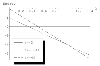
Figure 1: The lowest three eigenenergies of the $N=4$ case have been plotted as a function of the coupling constant $\lambda$. There are level crossings at $\lambda_{c,1}=\frac{1}{3}$ and at $\lambda_{c,2}=1$, which is in agreement with equation 16. The eigenenergies of the full system are $\epsilon={\pm 2,\pm 1-3\lambda,-4\lambda}$. The solid, short-dashed and long-short-dashed line correspond to the eigenenergies $\epsilon=-2$, $\epsilon=-1-3\lambda$ and $\epsilon=-4\lambda$, respectively.

We then construct the canonical partition function $\mathcal{Z}$ from the full set of eigenvalues. One can now determine the specific heat as given by the two equations 7-8.

IV.1 The analogous ”specific heat” $C^{*}_{\beta}$

Once the partition function has been constructed from the eigenvalues of the $N$-particle Hamiltonian, we are able to form the expectation value of the energy as given by the familiar canonical ensemble relation below.

$$\mathcal{E}=-\frac{\partial}{\partial\beta}\ln\mathcal{Z}$$ (29)

The quantity that will be used to map out the phase diagram of the model, which we will call $C^{*}_{\beta,\lambda}$, is given by the derivative of $\mathcal{E}$, with respect to either $\beta$ or $\lambda$. In this section we will focus our attention on the former case.

$$C^{*}_{\beta}=\frac{\partial}{\partial\beta}\mathcal{E(\beta,\lambda)}$$ (30)

A plot of $C^{*}_{\beta}$ is given in figure 2 for a fixed value of $\beta=110$. The value of $\beta$ was an arbitrary choice, in order to demonstrate the following point. At finite temperatures, that is when $\beta\neq\infty$, the peaks that are found in figure 2 are a signature of a phase transition taking place. They are smoothed out due to finite temperature effects. As the temperature is lowered ($\beta$ increases), the peaks move together and become smaller in size. This is shown in figure 3. When $\beta\rightarrow\infty$, the peaks around each critical point coalesce into a single point, namely $\lambda_{c}$. This is exactly what one would expect at zero temperature; the phase transition takes place where the eigenen-ergies become degenerate.

Figure 2: The quantity $C^{*}_{\beta}$ has been plotted as a function of the coupling constant $\lambda$, for the $N=4$ particle case, with a fixed value of $\beta=110$ (see text for a discussion on this point). There are two peaks present in the plot, centered around the two critical points $\lambda_{c}$ of the system. The peaks coalesce into a single point centered at $\lambda_{c}$ as $\beta\rightarrow\infty$ (see figure 3). Everywhere else $C^{*}_{\beta}=0$, in agreement with equation 9.

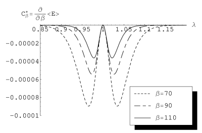
Figure 3: The temperature dependence of $C^{*}_{\beta}$ in the region of $\lambda_{c}=1$ for the $N=4$ particle case has been plotted. The short-dashed, long-short-dashed and solid peaks correspond to $\beta=70,90,110$ respectively. One can clearly see that as the temperature is lowered ($\beta\rightarrow\infty$), that the peaks become smaller in size and narrower in width. In the zero-temperature limit, these peaks would coalesce into a single point situated exactly at the location of the quantum phase transition.

IV.2 The analogous ”‘specific heat”’ $C^{*}_{\lambda}$

The above investigation of the quantity $C^{*}_{\beta}$ is one way to characterize the quantum phase transitions. It is also possible to investigate the qpt’s from another viewpoint. In this section we will consider the quantity $C^{*}_{\lambda}=\frac{\partial}{\partial\lambda}\mathcal{E(\beta,\lambda)}$.

In figure 4 we have plotted the dependence of $C^{*}_{\lambda}$ on $\beta$ for various values of $\lambda$. It can be seen that if the coupling constant is set in a range corresponding to one particular value of the ground state eigenenergy, that at low temperatures $C^{*}_{\lambda}$ tends to the value of the slope of the given eigenenergy. For example, when $0\leq\lambda<\frac{1}{3}$, $C^{*}_{\lambda}\rightarrow 0$ as $\beta$ becomes large. For that range of the coupling constant, the corresponding ground-state eigenvalue is $\epsilon=-2$, which of course has a slope of zero. Similarly for $\frac{1}{3}<\lambda<1$, $C^{*}_{\lambda}\rightarrow-3$, which corresponds to the slope of the ground state eigenvalue $\epsilon=-1-3\lambda$. At the critical values $\lambda_{c}$, $C^{*}_{\lambda}$ takes on the average value of the slope of the two degenerate eigenenergies involved. In figure 5, we have plotted the zero temperature limit of $C^{*}_{\lambda}$ as a function of $\lambda$. There are two discontinuities in the figure, corresponding to the values of $\lambda_{c}$ where the qpt takes place. The horizontal lines in the figure correspond to the slope of the current ground state eigenvalue.

Figure 4: $C^{*}_{\lambda}$ as a function of $\beta$ for various values of $\lambda$ for the $N=4$ particle case. The long-dashed curves (top two curves) correspond to $\lambda=0.1,0.2$; the medium-dashed curves correspond to $\lambda=0.5,0.75$ (in between the two solid curves); the short-dashed curves (lowest two curves) correspond to $\lambda=1.1,1.2$. The solid curves correspond to the the critical values of $\lambda_{c,n}=\frac{1}{3},1$. Curves that have same dashing style correspond to the same ground state eigenvalue and in the zero-temperature limit tend to the slope of that corresponding eigenvalue. At the critical points, $C^{*}_{\lambda}$ picks out the average value of the two slopes from the relevant degenerate eigenvalues.

Figure 5: $C^{*}_{\lambda}$ as a function of $\lambda$ in the zero-temperature limit for the $N=4$ particle case. The horizontal segments of the plot correspond to the derivatives (with respect to $\lambda$) of the ground state eigenvalue for that particular range of $\lambda$. For example, $\frac{1}{3}<\lambda<1$, $C^{*}_{\lambda}=-3$, which corresponds to the slope of the ground state eigenvalue $\epsilon=-1-3\lambda$. The discontinuities take place at the critical values of the system, viz $\lambda_{c,n}=\frac{1}{3},1$, respectively. At the qpt, the value of $C^{*}_{\lambda}$ is the average value of the two slopes of the relevant degenerate eigenvalues.

IV.3 The Plastino-Moszkowski model for $N=8$ particles.

It is also of interest to see if the above methodology works for a larger system. In this case the slope of the ground state energy as a function of the coupling constant does not change sign. We will briefly summarize the results when the model has $N=8$ particles present. Using equation 16, we determine that the critical coupling constants are the following values: $\lambda_{c,n}=\frac{1}{7},\frac{1}{5},\frac{1}{3},1$. For completeness, the 9 eigenvalues of the system are $\epsilon=\pm 4,\pm 1-15\lambda,\pm 2-12\lambda,\pm 3-7\lambda,-16\lambda$. The quantity $C^{*}_{\beta}$ is shown in figure 6 and is seen to correctly identify where the quantum phase transitions occur. In figure 7 we have plotted $C^{*}_{\lambda}$ in the zero-temperature limit as a function of $\lambda$. As in the $N=4$-particle case, the discontinuous jumps seen in the plot correspond to a quantum phase transition taking place.

Figure 6: $C^{*}_{\beta}$ has been plotted for $\beta=110$ (for illustration) in the $N=8$ particle case. The peaks are centered around the critical coupling constants $\lambda_{c,n}=\frac{1}{7},\frac{1}{5},\frac{1}{3}$. Recall that in the zero-temperature limit the peaks coalesce into a single point located at the critical points, as has been already shown for the $N=4$ particle case (see figure 3). Note that we have only plotted the first 3 critical points to make the plot clearer; the peak located at $\lambda_{c}=1$ is not shown.

Figure 7: $C^{*}_{\lambda}$ has been plotted in the zero-temperature limit for the $N=8$ particle case. The horizontal segments correspond to the derivative (with respect to $\lambda$) of the relevant ground state of the system for that particular range of $\lambda$. The discontinuities take place at the critical values of the coupling constant, viz $\lambda_{c,n}=\frac{1}{7},\frac{1}{5},\frac{1}{5},1$. At the qpt, the value of $C^{*}_{\lambda}$ is the average value of the two slopes of the relevant degenerate eigenvalues.

V Conclusions

We have here shown that classical phase transitions and quantum phase transitions can be described in a unified fashion. Our treatment has relied heavily on the specific heat and is also valid for finite systems where only the remnant of a classical phase transition exists. The pertinent considerations were illustrated in an exactly solvable model of Plastino and Moszkowski. In particular we have shown that information about qpt’s can be obtained from the quantity $\frac{\partial E_{gs}}{\partial\lambda}$ and that this equivalent to looking at the zero temperature limit of the specific heat.

References

- Sachdev (1999) S. Sachdev, Quantum Phase Transitions (Cambridge University Press, Cambridge, U.K., 1999).
- Davis and Miller (1987) E. D. Davis and H. G. Miller, Phys. Lett. B 196, 277 (1987).
- Alhassid and Zingman (1984) Y. Alhassid and J. Zingman, Phys. Rev C 30, 684 (1984).
- Egido et al. (1985) J. L. Egido, P. Ring, S. Iwasaki, and H. J. Mang, Phys. Lett. B 154, 1 (1985).
- Goodman (1984) A. L. Goodman, Phys. Rev. C 29, 1887 (1984).
- Jaynes (1957a) E. T. Jaynes, Phys. Rev. 106, 620 (1957a).
- Jaynes (1957b) E. T. Jaynes, Phys. Rev. 108, 171 (1957b).
- Plastino and Moszkowski (1978) A. Plastino and S. A. Moszkowski, Il Nueovo Cimento 47A, 470 (1978).
- Dicke (1954) R. H. Dicke, Phys. Rev. 93, 99 (1954).
- Lipkin et al. (1965) H. J. Lipkin, N. Meshkov, and A. J. Glick, Nucl. Phys. 62, 188 (1965).