A first step to Convolutive Sparse Representation

Abstract

In this paper an extension of the sparse decomposition problem is considered and an algorithm for solving it is presented. In this extension, it is known that one of the shifted versions of a signal ${\bf s}$ (not necessarily the original signal itself) has a sparse representation on an overcomplete dictionary, and we are looking for the sparsest representation among the representations of all the shifted versions of ${\bf s}$. Then, the proposed algorithm finds simultaneously the amount of the required shift, and the sparse representation. Experimental results emphasize on the performance of our algorithm.

Index Terms—  atomic decomposition, sparse decomposition, sparse representation, overcomplete signal representation, sparse source separation

1 Introduction

In the classical atomic decomposition problem [1], we have a signal $s(t)$ whose samples are collected in the $n\times 1$ signal vector ${\bf s}=[s(1),\dots,s(n)]^{T}$ and we would like to represent it as a linear combination of $m$, $n\times 1$ signal vectors $\{{\mbox{\boldmath$\varphi$}}_{i}\}_{i=1}^{m}$. After [2], the vectors ${\mbox{\boldmath$\varphi$}}_{i}$, $1\leq i\leq m$ are called atoms and they collectively form a dictionary over which the signal is to be decomposed. We may write

$${\bf s}=\sum_{i=1}^{m}\alpha_{i}{\mbox{\boldmath$\varphi$}}_{i}={\mbox{\boldmath{$\Phi$ }}}{\mbox{\boldmath$\alpha$}},$$ (1)

where ${\mbox{\boldmath{$\Phi$ }}}\triangleq[{\mbox{\boldmath$\varphi$}}_{1},\dots,{\mbox{\boldmath$\varphi$}}_{m}]$ is the $n\times m$ dictionary (matrix) and ${\mbox{\boldmath$\alpha$}}\triangleq(\alpha_{1},\dots,\alpha_{m})^{T}$ is the $m\times 1$ vector of coefficients. A dictionary with $m>n$ is called overcomplete. Although, $m=n$ is sufficient to obtain such a decomposition (like what is done in Discrete Fourier Transform), using overcomplete dictionaries has a lot of advantages in many diverse applications (refer for example to [3] and the references in it). Note that for the overcomplete case, the representation is not unique, but all these applications need a sparse representation, that is, the signal ${\bf s}$ should be represented as a linear combination of as small as possible number of atoms of the dictionary. It has been shown [4, 5] that with some mild conditions on the dictionary matrix, if there is a sparse representation with at most $n/2$ non-zero coefficients, then this representation is unique. The main approaches for finding this sparse solution include Matching Pursuit (MP) [2, 6], FOCUSS [5], Basis Pursuit (BP) [1], and Smoothed $\ell^{0}$ (SL0) [7].

In this paper, we introduce a generalization of this classical problem to the case that we call ‘convolutive sparse representation’. In this case, it is known that the signal ${\bf s}$ has a sparse representation not over the dictionary itself, but over some (unknown) shifted versions of the atoms. To state the problem more clearly, consider a representation of the form:

$${\bf s}=\sum_{i=1}^{m}\alpha_{i}{{{\mbox{\boldmath$\varphi$}}}_{i}}^{(k_{i})},$$ (2)

where ${{{\mbox{\boldmath$\varphi$}}}_{i}}^{(k_{i})}$ stands for the $k_{i}$-sample (circularly) shifted version of ${\mbox{\boldmath$\varphi$}}_{i}$. Then, our problem is to find the sparsest representation in the form of (2) among all the possible values for $k_{1},\dots,k_{m}$.

Note also that the Fourier transform does not convert this problem to the classical sparse representation (1) in the frequency domain: The problem in the transformed domain will be similar to (1), but with time varying $\alpha_{i}$’s.

In this paper, we address only a special case of the general problem (2), that is, where all the shifts $k_{i}$ are equal. This is equivalent to this simplified problem: an unknown shifted version of ${\bf s}$ has a sparse representation over the dictionary, and we would like to find this representation.

One of the trivial applications of the general problem is to reduce the size of the dictionary in atomic decomposition applications. An example for the applications of the above simplified problem is where our recorded signal, which has to be decomposed as a combination of a small number of atoms of the dictionary, is shifted relative to its underlying atoms that already exist in the dictionary.

The paper organized as follows. In Section 2 the main idea of the algorithm is introduced. The resulting algorithm is then stated in Section 3. Finally, simulation results of the algorithm are presented in Section 4.

2 Main Idea

Consider a dictionary with atoms ${{\mbox{\boldmath$\varphi$}}}_{1},{{\mbox{\boldmath$\varphi$}}}_{2},\cdots,{{\mbox{\boldmath$\varphi$}}}_{m}$. The problem is then to sparsely decompose an $n\times 1$ vector  ${\bf s}$ as a linear combination of shifted atoms of the dictionary (in this paper, the shifts are assumed to be circular). One trivial solution to the problem is to insert all shifted atoms in the dictionary and then find the sparsest representation of the vector ${\bf s}$ for that dictionary using the conventional atomic decomposition methods. However, this direct solution demands a high computational and storage load.

Let also that $k_{i}$ be a continuous variable (a non-integer shift $k_{i}$ can be imagined as shifting the hull of signal and then re-sampling it). For handling circular shifts more easily, we take the Discrete Fourier Transform (DFT) of both sides of (2) to obtain:

$${\bf s^{\cal{(F)}}}=\sum_{i=1}^{m}\alpha_{i}{\bf W}_{i}{{\mbox{\boldmath$\varphi$}}}_{i}^{\cal{(F)}}$$ (3)

in which ${\bf s^{\cal{(F)}}}$ and ${\mbox{\boldmath$\varphi$}}_{i}^{\cal{(F)}}$ are the DFTs of the signals ${\bf s}$ and ${\mbox{\boldmath$\varphi$}}_{i}$ repectively, and

$${\bf W}_{i}\triangleq\left(\begin{array}[]{c c c c c}{w_{i}}^{0}&0&0&0&0\\ 0&{w_{i}}^{1}&0&0&0\\ 0&0&{w_{i}}^{2}&0&0\\ 0&0&0&\ddots&0\\ 0&0&0&0&{w_{i}}^{n-1}\end{array}\right),w_{i}\triangleq e^{-j\frac{2\pi}{n}k_{i}}$$

As stated in the introduction, in this paper we consider only the case in which $w_{1}=w_{2}=\cdots=w_{m}$, and we present an iterative algorithm to solve the problem in this case. This case is equivalent to assuming that the atoms of the dictionary are fixed and the signal ${\bf s}$ is shifted in opposite direction. In this case:

$${\bf W}_{1}={\bf W}_{2}=\cdots={\bf W}_{m}={\bf W},$$

and hence from (3) we have:

$${\bf s^{\cal{(F)}}}={\bf W}\sum_{i=1}^{m}\alpha_{i}{\mbox{\boldmath$\varphi$}}_{i}^{\cal{(F)}}$$ (4)

or:

$${\bf W}^{\prime}{\bf s^{\cal{(F)}}}=\sum_{i=1}^{m}\alpha_{i}{\mbox{\boldmath$\varphi$}}_{i}^{\cal{(F)}}={\mbox{\boldmath{$\Phi$ }}}^{\cal{(F)}}{\mbox{\boldmath$\alpha$}}$$ (5)

where:

$${\bf W}^{\prime}={\bf W}^{-1}=\left(\begin{array}[]{c c c c c}{{w^{\prime}}}^{0}&0&0&0&0\\ 0&{{w^{\prime}}}^{1}&0&0&0\\ 0&0&{{w^{\prime}}}^{2}&0&0\\ 0&0&0&\ddots&0\\ 0&0&0&0&{{w^{\prime}}}^{n-1}\end{array}\right)\\$$

in which ${w^{\prime}}=e^{j\frac{2\pi}{n}k}$. Now the problem is to find the sparsest solution of (5). To do so, we should have some criterion $F({\mbox{\boldmath$\alpha$}})$ for sparseness of the solution vector $\alpha$ and optimize that criterion subject to the constraint (5) using optimization methods. Note also that one of the unknows, $k$ does not exist in the objective function $F({\mbox{\boldmath$\alpha$}})$, and appears only in the constraint (5). As their objective functions, two classical sparse decomposition approaches use $\ell^{1}$-norm [1], and smoothed $\ell^{0}$ (SL0) norm [7]. Here we use the second one, because it results in a very fast and accurate algorithm in classical atomic decomposition [7], and also because it is a differentiable measure of the sparsity of $\alpha$. Smoothed $\ell^{0}$-norm of a vector is an approximation to its $\ell^{0}$-norm (number of its non-zero element), and is defined as:

$$F({\mbox{\boldmath$\alpha$}})=m-\sum_{i=1}^{m}{e^{-{\alpha_{i}}^{2}/{2\sigma^{2}}}}$$ (6)

where $\sigma$ is a parameter which specifies a tradeoff between smoothness and the accuracy of approximation: the smaller $\sigma$, the better approximation of the $\ell^{0}$ norm; the larger $\sigma$, the smoother objective function.

On the other hand, (5) can be written as:

$$G({\mbox{\boldmath$\alpha$}},w^{\prime})=\|{\bf W}^{\prime}{\bf s^{\cal{(F)}}}-{\mbox{\boldmath{$\Phi$ }}}^{\cal{(F)}}{\mbox{\boldmath$\alpha$}}\|^{2}=0$$ (7)

Now we should minimize (6) subject to the (7), for a small value of $\sigma$. Note that one of the optimization variables ($w^{\prime}$), is not present in $F({\mbox{\boldmath$\alpha$}})$, and appears only in (7).

Note that for small values of $\sigma$, $F$ contains a lot of local minima. Consequently, it is very difficult to directly minimize this function for very small values of $\sigma$. The idea of [7] for escaping from local minima is then to decrease the value of $\sigma$ gradually: for each value of $\sigma$ the minimization algorithm is initiated with the minimizer of the $F$ for the previous (larger) value of $\sigma$. This idea of minimizing a non-convex function is called Graduated Non-Convexity [8], and is also used in simulated annealing methods.

To start the minimization, we should find a proper initial guess for the solution ${\mbox{\boldmath$\alpha$}}_{0}$, that is, the initial estimation of the sparsest solution of ${\mbox{\boldmath{$\Phi$ }}}{\mbox{\boldmath$\alpha$}}={\bf s}$. It has been shown that for the case of the simple sparse decomposition, the best initial value for $\alpha$ is the minimum $\ell^{2}$-norm solution of ${\mbox{\boldmath{$\Phi$ }}}{\mbox{\boldmath$\alpha$}}={\bf s}$, that is, ${\mbox{\boldmath$\alpha$}}_{0}={\mbox{\boldmath{$\Phi$ }}}^{T}({\mbox{\boldmath{$\Phi$ }}}{\mbox{\boldmath{$\Phi$ }}}^{T})^{-1}{\bf s}$ [7]. The reason is that this solution minimizes the function $F({\mbox{\boldmath$\alpha$}})$ subject to ${\mbox{\boldmath{$\Phi$ }}}{\mbox{\boldmath$\alpha$}}={\bf s}$ where $\sigma$ goes to infinity. Despite the fact that our method is somehow different with the method presented in [7], we use the same initialization for our algorithm. Since we also have the variable $w^{\prime}$, we should start from the sparsest ${\mbox{\boldmath$\alpha$}}(k)={\mbox{\boldmath{$\Phi$ }}}^{T}({\mbox{\boldmath{$\Phi$ }}}{\mbox{\boldmath{$\Phi$ }}}^{T})^{-1}{\bf s}^{(k)}$ vector. Let $k_{0}=\mathop{\textrm{argmin}}_{k}F({\mbox{\boldmath$\alpha$}}(k))$, for $k=1,2,\dots,n$. Then we choose ${\mbox{\boldmath$\alpha$}}(k_{0})$ to be the starting point of our algorithm.

Because of noise, if our algorithm tries to satisfy (7) exactly, it would be very sensitive to noise. Consequently, we try to satisfy this equation approximately. We realize this idea by minimizing the function $H$ defined below with respect to $\alpha$ and ${w^{\prime}}$:

$$H({\mbox{\boldmath$\alpha$}},w^{\prime})=\lambda G({\mbox{\boldmath$\alpha$}},w^{\prime})+(1-\lambda)F({\mbox{\boldmath$\alpha$}})$$ (8)

where $0<\lambda<1$ is a constant that specifies the weight which is given to satisfying (7). This equation can be interpreted as a trade-off between the accuracy of the decomposition and maximizing the sparsity.

By letting $w^{\prime}=e^{j\theta}$, the final objective function $H({\mbox{\boldmath$\alpha$}},\theta)$ will be a real-valued function of real-valued variables $\alpha$ and $\theta$. For each $\sigma$, this function may be minimized by gradient based algorithms (specifically steepest descent). Direct calculations show:

$$\begin{split}\frac{\partial H}{\partial{\mbox{\boldmath$\alpha$}}}&=2\lambda\Re\{{\mbox{\boldmath{$\Phi$ }}}^{\cal{(F)}\mathrm{T}}({\mbox{\boldmath{$\Phi$ }}}^{\cal{(F)}}{\mbox{\boldmath$\alpha$}}-{\bf W}^{\prime}{\bf s^{\cal{(F)}}})\}+\\ &(1-\lambda)(1/\sigma^{2})[\alpha_{1}e^{(-\alpha_{1}^{2}/2\sigma^{2})},\dots,\alpha_{m}e^{(-\alpha_{m}^{2}/2\sigma^{2})}]^{T}\end{split}$$ (9)

$$\frac{\partial H}{\partial\theta}=-2\Re\{{\bf s^{\cal{(F)}}}{\bf M}{\bf W}^{\prime}{\mbox{\boldmath$\bar{\Phi}$}}\}$$ (10)

where ${\bf M}\triangleq\mathrm{diag}(0,1j,\dots,(n-1)j)$.

3 The Final Algorithm

The final algorithm of the proposed method is given in Fig. 1. As seen in the algorithm, the final values of the previous estimation are used for initialization of the next steepest descent. As explained in the previous section, the decreasing sequence of $\sigma$ is used to escape from getting trapped into local minima.

In the minimization part, the steepest descent with variable step-size ($\mu$) has been used: If $\mu$ is such that $H({\mbox{\boldmath$\alpha$}}-\mu\frac{\partial H}{\partial{\mbox{\boldmath$\alpha$}}},\theta-\mu\frac{\partial H}{\partial\theta})<H({\mbox{\boldmath$\alpha$}},\theta)$ we multiply the value of $\mu$ by 1.2 for the next iteration. Otherwise if $\mu$ is such that $H({\mbox{\boldmath$\alpha$}}-\mu\frac{\partial H}{\partial{\mbox{\boldmath$\alpha$}}},\theta-\mu\frac{\partial H}{\partial\theta})\geq H({\mbox{\boldmath$\alpha$}},\theta)$ we multiply the value of $\mu$ by 0.5 for the next iteration.

    • Initialization: 1. Let: $F({\mbox{\boldmath$\alpha$}})=m-\sum_{i=1}^{m}{e^{-{\alpha_{i}}^{2}/{2\sigma^{2}}}}$ and ${\mbox{\boldmath$\alpha$}}(k)={\mbox{\boldmath{$\Phi$ }}}^{T}({\mbox{\boldmath{$\Phi$ }}}{\mbox{\boldmath{$\Phi$ }}}^{T})^{-1}{\bf s}^{(k)}$. 2. Find the minimum of $F({\mbox{\boldmath$\alpha$}}(k))$ for $k=1,2,\cdots,n$. Assuming this minimum occurs for $k=k_{0}$, let ${\mbox{\boldmath$\hat{\alpha}$}}_{0}={\mbox{\boldmath$\alpha$}}(k_{0})$ and $\hat{\theta}_{0}=\frac{2\pi}{n}k_{0}$. 3. Choose a suitable decreasing sequence for $\sigma=[\sigma_{1}\ldots\sigma_{R}]$. Choose a small value for $\mu$. 4. Let ${\bf M}=\mathrm{diag}(0,1j,\dots,(n-1)j)$. • For $r=1,\dots,R$: 1. Let $\sigma=\sigma_{r}$. 2. Minimize (approximately) the function $H({\mbox{\boldmath$\alpha$}},\theta)$ using $L$ iterations of the steepest descent algorithm: – Initialization: ${\mbox{\boldmath$\alpha$}}={\mbox{\boldmath$\hat{\alpha}$}}_{r-1}$ and $\theta=\hat{\theta}_{r-1}$. – for $l=1\dots L$ (loop $L$ times): (a) Calculate $\frac{\partial H}{\partial{\mbox{\boldmath$\alpha$}}}$ and $\frac{\partial H}{\partial\theta}$ from (9) and (10), respectively. (b) If $H({\mbox{\boldmath$\alpha$}}-\mu\frac{\partial H}{\partial{\mbox{\boldmath$\alpha$}}},\theta-\mu\frac{\partial H}{\partial{\mbox{\boldmath$\alpha$}}})<H({\mbox{\boldmath$\alpha$}},\theta)$ let $\rho=1.2$ else $\rho=0.5$. (c) Let ${\mbox{\boldmath$\alpha$}}\leftarrow{\mbox{\boldmath$\alpha$}}-\mu{\partial H}/{\partial{\mbox{\boldmath$\alpha$}}}$
and $\theta\leftarrow\theta-\mu{\partial H}/{\partial\theta}$. (d) Let $\mu\leftarrow\mu\times\rho$. 3. Set ${\mbox{\boldmath$\hat{\alpha}$}}_{r}={\mbox{\boldmath$\alpha$}}$ and $\hat{\theta}_{r}=\theta$. • Let ${\mbox{\boldmath$\hat{\alpha}$}}={\mbox{\boldmath$\hat{\alpha}$}}_{R}$ and $\hat{\theta}=\hat{\theta}_{R}$. The final coefficient vector is $\hat{\alpha}$ and the final shift value is $n\times\frac{\hat{\theta}}{2\pi}$.    

Fig. 1: The final algorithm

4 EXPERIMENTAL RESULTS

In order to experimetally evaluate our method, we generated a random dictionary $\Phi$ which had $80$ atoms and each atom was a signal of length $40$ (thus we assumed $m=80$ and $n=40$ in our simulations). Then we created a synthetic vector ${\bf s}$ by generating a sparse coefficient vector $\alpha$ at random, using a Bernoulli-Gaussian model: each coefficient is ‘active’ with probability $p$, and is ‘inactive’ with probability $1-p$. If it is active, its value is modeled by a zero-mean Gaussian random variable with variance $\sigma^{2}_{\mathrm{on}}$; if it is not active, its value is modeled by a zero-mean Gaussian random variable with variance $\sigma^{2}_{\mathrm{off}}$, where $\sigma^{2}_{\mathrm{off}}\ll\sigma^{2}_{\mathrm{on}}$. Consequently, each $\alpha_{i}$ is distributed as:

$$\alpha_{i}\sim p\cdot\mathcal{N}(0,\sigma_{\mathrm{on}})+(1-p)\cdot\mathcal{N}(0,\sigma_{\mathrm{off}}),$$ (11)

where $p$ denotes the probability of activity of the coefficient, and sparsity implies that $p\ll 1$. In our simulations we have fixed $\sigma_{\mathrm{on}}=1,\sigma_{\mathrm{off}}=0.01$, $p=0.1$, and $\lambda=0.75$.

Then we created the signal ${\bf s}$ by ${\bf s}={\mbox{\boldmath{$\Phi$ }}}{\mbox{\boldmath$\alpha$}}+{\bf n}$, where $\bf n$ is an additive white Gaussian noise with zero mean and standard deviation $\sigma_{\mathrm{n}}=0.01$. Finally, we shifted the ${\bf s}$ vector circularly by $k$ samples where $k$ was a random number from $0$ to $39$. We applied our algorithm to convolutively decompose this vector ${\bf s}$ over the dictionary $\Phi$ .

The simulation was repeated 1000 times with randomly generated coefficients, dictionary and the shift of the signal, and it was seen that in 992 experiment the algorithm could sucessfully estimate the shift value and the coefficient vector $\alpha$. In average, the Signal to Noise Ratio (SNR) was greater than 24dB. Figure 2 shows one of the runs of these experiments. In the other 8 experiments the algorithm felled into local minima, and could not correctly estimated $\alpha$ and $\theta$.

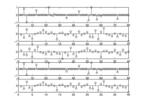
Fig. 2: A sample of our experiments. From top to bottom, first plot represents a randomly generated coefficient vector $\alpha$, second plot is the synthetic vector ${\bf s}$ which has the coefficient vector $\alpha$ on the randomly generated dictionary $\Phi$ , third plot is a randomly shifted version of vector ${\bf s}$ which is the input of our algorithm, fourth plot is the estimated coefficient vector $\hat{\alpha}$, and the last plot is the vector $\hat{\bf s}$ which has the coefficient vector $\hat{\alpha}$.

In order to see the effect of $\lambda$ on the estimation quality, the algorithm was repeated for $\lambda$’s between 0.3 and 0.9 (outside this interval SNR decreases rapidly). For each value of $\lambda$ we repeated the algorithm 100 times and the mean SNR for each $\lambda$ is computed. The mean SNR is plotted versus $\lambda$ in Fig. 3.

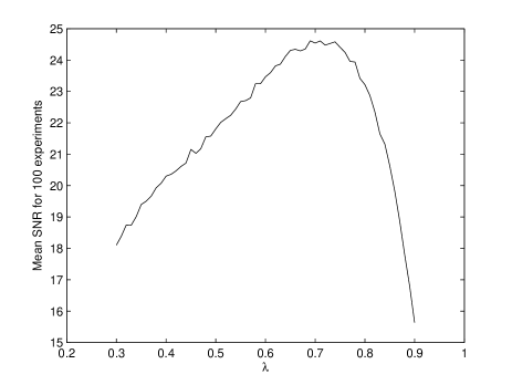
Fig. 3: Output SNR versus $\lambda$.

5 CONCLUSION

In this paper, a new method was proposed as the first step for solving the convolutive sparse decomposition problem. The proposed method can be used in the cases in which we know that one of the shifted versions of a signal ${\bf s}$ has a sparse representation on an overcomplete dictionary, and we are looking for the sparsest representation among the representations of all the shifted versions of ${\bf s}$. We used Discrete Fourier Transform (DFT) to convert the problem to a continuous optimization problem. The proposed method was fast because of using the idea of smoothed $\ell^{0}$-norm [7]. Experimental results emphasized on the performance of the proposed algorithm.

It seems that the proposed algorithm can be generalized for applying to the general convolutive sparse representation problem (in which the shift values $k_{i}$ are not necessarily equal). However, our simulations show that the main difficulty of such a generalization is that the algorithm very oftenly traps into local minima. Such a generalization is currently under study in our group.

References

- [1] S. S. Chen, D. L. Donoho, and M. A. Saunders, “Atomic decomposition by basis pursuit,” SIAM Journal on Scientific Computing, vol. 20, no. 1, pp. 33–61, 1999.
- [2] S. Mallat and Z. Zhang, “Matching pursuits with time-frequency dictionaries,” IEEE Trans. on Signal Proc., vol. 41, no. 12, pp. 3397–3415, 1993.
- [3] D. L. Donoho, M. Elad, and V. Temlyakov, “Stable recovery of sparse overcomplete representations in the presence of noise,” IEEE Trans. Info. Theory, vol. 52, no. 1, pp. 6–18, Jan 2006.
- [4] D. L. Donoho, “For most large underdetermined systems of linear equations the minimal -norm solution is also the sparsest solution,” Tech. Rep., 2004.
- [5] I. F. Gorodnitsky and B. D. Rao, “Sparse signal reconstruction from limited data using FOCUSS, a re-weighted minimum norm algorithm,” IEEE Transactions on Signal Processing, vol. 45, no. 3, pp. 600–616, March 1997.
- [6] S. Krstulovic and R. Gribonval, “MPTK: Matching pursuit made tractable,” in ICASSP’06, 2006.
- [7] G.H. Mohimani, M. Babaie-Zadeh, and C. Jutten, “Fast sparse representation based on smoothed -norm,” in ICA2007, London, September 2007.
- [8] A. Blake and A. Zisserman, Visual Reconstruction, MIT Press, 1987.