Nicest, a near-infrared color excess method tailored for small-scale structures.

Observational data and theoretical calculations show that significant small-scale substructures are present in dark molecular clouds. These inhomogeneities can provide precious hints on the physical conditions inside the clouds, but can also severely bias extinction measurements. We present Nicest, a novel method to account and correct for inhomogeneities in molecular cloud extinction studies. The method, tested against numerical simulations, removes almost completely the biases introduced by sub-pixel structures and by the contamination of foreground stars. We applied Nicest to 2MASS data of the Pipe molecular complex. The map thereby obtained shows significantly higher (up to $0.41\mbox{ mag}$ in $A_{K}$) extinction peaks than the standard Nicer (Lombardi et al. 2001) map. This first application confirms that substructures in nearby molecular clouds, if not accounted for, can significantly bias extinction measurements in regions with $A_{K}>1\mbox{ mag}$; the effect, moreover, is expected to increase in more distant molecular cloud, because of the poorer physical resolution achievable.

1 Introduction

Although the details of star and planet formation are very little known, there is a large consensus that these objects are created inside dark molecular clouds from the contraction and fragmentation of dense, cold cores. As a result, in the last decades molecular clouds have been studied in detail using many different techniques, from optical number counts (Wolf, 1923; Bok, 1937), to radio observations of carbon monoxide (CO) molecules (Wilson et al., 1970; Frerking et al., 1982), to near-infrared (NIR) extinction measurements (Lada et al., 1994).

Molecular hydrogen and helium represent approximately $99\%$ of the mass of a cloud, but the absence of a dipole moment in these molecules makes them virtually undetectable at the low temperatures ($T\sim 10\mbox{ K}$) present in these objects. Hence, the (projected) mass distribution of dark clouds is usually inferred from the distribution of relatively rare tracers (such as CO or dust grains) under the assumption that these are uniformly distributed in the cloud.

As pointed out by Lada et al. (1994), the reddening of background stars in NIR bands is a simple and reliable method to study the dust distribution and thus the hydrogen column density. Compared to optical bands, NIR bands are less affected by extinction and are less sensitive to the physical properties of the dust grains (Mathis, 1990), and thus their color excess can be directly translated into a hydrogen column density. In a series of papers we reconsidered and improved the NIR color excess (Nice) technique, by generalizing it to use three or more bands (Nicer, see Lombardi & Alves, 2001) and by taking a maximum-likelihood approach (Lombardi, 2005).

Although the Nice and Nicer techniques have been very successful in studying molecular clouds (see, e.g., Alves et al., 2001), they are plagued by two complications: small-scale inhomogeneities and contamination by foreground stars. NIR studies typically assume a uniform extinction over (small) patches of the sky; however, in presence of substructures such as steep gradients, unresolved filaments, or turbulence-induced inhomogeneities (Lada et al., 1994; Larson, 1981; Heyer & Brunt, 2004), the background stars used to estimate the cloud extinction would not be uniformly distributed in the patch, but would be preferentially observed in low density regions. Similarly, in presence of foreground stars, their relative fraction increases with the dust column density. Unfortunately, both effects will bias all color excess estimators toward low column densities; moreover, the bias will be especially important in the dense regions of molecular clouds, which is where the star formation takes place.

In this paper we describe in details the repercussions of small scale inhomogeneities and foreground stars in extinction measurements, and propose a simple method to obtain estimates of the column density in presence of both effects that, under simple working hypotheses, is asymptotically unbiased. Our method does not rely on any (usually poorly verified) assumption regarding the small scale structure of the cloud; moreover, it can be applied to a general class of NIR extinction measurements (marked spatial point processes).

The paper is organized as follows. In Sect. 2 we introduce a general smoothing technique virtually used in all cases to create smooth, continuous maps from the discrete pencil-beam extinction measurements carried out for each background star; we also show that in two typical applications (moving average and nearest neighbours smoothing) a bias is expected. In Sect. 3 we propose a new method that can correct this bias without making any assumption on the underlying form of the cloud substructure. This new method has been tested with numerical simulations, as described in Sect. 4, and with a real-case application, presented in Sect. 5. We discuss and comment the results obtained in Sect. 6, and finally we briefly present our conclusions in Sect. 7.

2 Cloud substructure

Measurements of the reddening of stars observed through a molecular cloud provide estimates of the cloud column densities on pencil beams characterized by a diameter of the order of a fraction of milliarcsec. However, these high resolution measurements are strongly undersampled and are affected by large uncertainties due to the photometric errors and to the intrinsic scatter of star colors in the NIR. Smooth and continuous extinction maps are normally obtained by interpolating and binning the various pencil beams. Different authors use different recipes to smooth the data (see, e.g., Lombardi, 2002 for a description of several interpolation techniques), but in most cases the interpolation follows a standard scheme. Consider $N$ $K$-band extinction measurements $\bigl{\{}\hat{A}_{n}\bigr{\}}$ obtained, for example, from the color excess of $N$ background (see Lada et al., 1994 or Lombardi & Alves, 2001). The extinction $\hat{A}$ at any location in the sky is evaluated using a weighted average

$$\hat{A}=\frac{\sum_{n}w_{n}\hat{A}_{n}}{\sum_{n}w_{n}}\;.$$ (1)

The weights $\{w_{n}\}$ are usually chosen to be significantly different from zero only for stars angularly close to the given location of the map (for example, Cambrésy et al., 2002 assign a unity weight to the $N$ nearest neighbors). Clearly, Eq. (1) does not include slightly more complex situations where, for example, one takes the median of the extinctions measured from objects nearby a given position (e.g. Dobashi et al., 2008); however, most of the discussion carried out for the weighted average actually applies also to median or related estimators.

The binning in Eq. (1) washes out the cloud substructure on scales smaller than the typical size where the $\{w_{n}\}$ are significantly different from zero, but this is needed in order to have smooth maps and to increase the signal-to-noise ratio. However, Eq. (1) also introduces a significant bias on the estimated column density. Suppose that, in the region of the sky that we are investigating (i.e., in the area covered by the $N$ stars used to estimate $A$) the column density has significant variations. Because of this, the local density $\rho(\@vec{x})$ of stars is not homogeneous though the cloud, but rather follows the scheme

$$\rho(\@vec{x})=\rho_{0}10^{-\alpha k_{\lambda}A(\@vec{x})}\;,$$ (2)

where $\rho_{0}$ is the density of stars where no extinction is present, $\alpha$ is the slope of the number counts, and $k_{\lambda}=A_{\lambda}/A$ is the extinction law in the band $\lambda$ considered. This effect, which is at the origin of the historical number count method to measure column densities in molecular clouds (Wolf, 1923; Bok, 1937), also induces a bias in Eq. (1), since regions with smaller extinctions and thus higher density of background stars will, on average, contribute more to the sum in Eq. (1) than regions with large extinctions. Note that since the color excess method requires measurements in at least two different bands, one should replace Eq. (2) with a version that provides the expected density of stars observed in all bands required for the application of the method (e.g., $H$ and $K$). For equally deep observations on all bands, the result has the same form of Eq. (2), where $k_{\lambda}$ is the extinction law of the bluer band considered (e.g., $H$).

The main issue considered in this paper is the bias introduced by unresolved substructures in Eq. (1). In general, the bias should be defined here as the difference between the expected, mean value of $\langle\hat{A}\rangle$ and the true column density $A$ at the same position. However, clearly every smoothing technique introduces a bias because of the smoothing itself, and this bias is normally acceptable if it does not introduces a systematic effect on the total column density. In other words, a required property is

$$\int A(\@vec{x})\,\mathrm{d}x=\left\langle\int\hat{A}(\@vec{x})\,\mathrm{d}x\right\rangle=\int\bigl{\langle}\hat{A}(\@vec{x})\bigr{\rangle}\,\mathrm{d}x\;.$$ (3)

Clearly, in order for Eq. (3) to hold, the difference $\langle\hat{A}\rangle-A$ must be of alternating sign. For our purposes, thus, it is more useful to define the bias as the difference between the expected mean value $\langle\hat{A}\rangle$ and the same quantity that we would theoretically expect in presence of a uniform density of stars, i.e. by ignoring the dependence of the density of stars on the local extinction described by Eq. (2) [see also below Eq. (7)]. This definition is useful, since it isolates the standard effects of a smoothing from the effects introduced by the non-uniform sampling of the cloud structure. In addition, a column density estimator $\hat{A}(\@vec{x})$ that is unbiased according to this definition will also be unbiased according to Eq. (3) (provided the weights $w_{n}$ are spatially invariant). For, when the density of background stars is uniform, $\bigl{\langle}\hat{A}(\@vec{x})\bigr{\rangle}$ can always be written as a convolution of the true column density map $A(\@vec{x})$ with some kernel $K$ normalized to unity (Lombardi, 2002).

In the following, we will calculate explicitly this bias in two common smoothing schemes.

2.1 Moving average smoothing

In this section we will consider a simple weighting scheme in Eq. (1) where each weight $w_{n}=w(\@vec{x}_{n};\@vec{x})$ is a simple function of the location $\@vec{x}_{n}$ of the $n$-th star (typically, $w(\@vec{x}_{n};\@vec{x}_{n})$ will depend only on the modulus $\lvert\@vec{x}_{n}-\@vec{x}\rvert$).

As discussed above, our aim is to compare the expected column density estimate with the one that we would obtain in absence of any selection effect in the number of background stars. We need thus to evaluate two averages: (i) $\bigl{\langle}\hat{A}(\@vec{x})\bigr{\rangle}$, where $\hat{A}$ is calculated according to Eq. (1) and the ensemble average is taken over all positions of stars with the density given by Eq. (2) and over all individual column density measurements $\hat{A}_{n}$; and (ii) the average $\bar{A}(\@vec{x})$, which is basically the same quantity evaluated with a constant density of background stars $\rho_{0}$.

In principle, both averages can be calculated analytically using the method described by Lombardi & Schneider (2001; see below Sect. 3); in practice, for the purposes of this section a simple approximation can be used provided that in the weighted average of Eq. (1) a relatively large number of column densities are used with weights significantly different from 0. In this case we find for the first average

$$\bigl{\langle}\hat{A}(\@vec{x})\bigr{\rangle}=\frac{\int A(\@vec{x}^{\prime})w(\@vec{x}^{\prime};\@vec{x})\rho(\@vec{x}^{\prime})\,\mathrm{d}x^{\prime}}{\int w(\@vec{x}^{\prime};\@vec{x})\rho(\@vec{x}^{\prime})\,\mathrm{d}x^{\prime}}\;.$$ (4)

As shown by Eq. (2), $\rho(\@vec{x}^{\prime})$ is a simple function of $A(\@vec{x}^{\prime})$. This suggests that the equation can be recast in a simpler form by defining $p_{A}(A;\@vec{x})$, the (weighted) probability that a point with extinction $A$ is used to evaluate $\hat{A}(\@vec{x})$, the column density at $\@vec{x}$:

$$p_{A}(A;\@vec{x})=\frac{\int w(\@vec{x}^{\prime};\@vec{x})\delta\bigl{(}A-A(\@vec{x}^{\prime})\bigr{)}\,\mathrm{d}x^{\prime}}{\int w(\@vec{x}^{\prime};\@vec{x})\,\mathrm{d}x^{\prime}}\;.$$ (5)

By using Eq. (5) in Eq. (4) we find then

$$\bigl{\langle}\hat{A}(\@vec{x})\bigr{\rangle}=\frac{\int Ap_{A}(A;\@vec{x})\rho(A)\,\mathrm{d}A}{\int p_{A}(A;\@vec{x})\rho(A)\,\mathrm{d}A}=\frac{\int Ap_{A}(A;\@vec{x})10^{-\alpha k_{\lambda}A}\,\mathrm{d}A}{\int p_{A}(A;\@vec{x})10^{-\alpha k_{\lambda}A}\,\mathrm{d}A}\;.$$ (6)

In presence of a uniform distribution of stars, $\rho(\@vec{x})=\rho_{0}$, we would instead obtain simply

$$\bar{A}(\@vec{x})=\frac{\int A(\@vec{x}^{\prime})w(\@vec{x}^{\prime};\@vec{x})\,\mathrm{d}x^{\prime}}{\int w(\@vec{x}^{\prime};\@vec{x})\,\mathrm{d}x^{\prime}}=\int Ap_{A}(A;\@vec{x})\,\mathrm{d}A\;.$$ (7)

The two values presented in Eqs. (6) and (7) do not differ significantly provided the scatter of $A$ in the patch considered around $\@vec{x}$ is much smaller than $(\alpha k_{\lambda}\ln 10)^{-1}$. For example, if we consider the $H$ band of a typical region close to the Galactic plane with a standard reddening law (Rieke & Lebofsky, 1985), we have $\alpha\simeq 0.34\mbox{ mag}^{-1}$ and $k_{H}\simeq 1.55$ (Indebetouw et al., 2005), so that the maximum scatter allowed in $A_{K}$ to have a negligible bias is${}\ll 0.82\mbox{ mag}$. Hence, clearly we need to be concerned by this bias in regions from moderate to large extinction.

It is also interesting to evaluate the bias $\bigl{\langle}\hat{A}(\@vec{x})\bigr{\rangle}-\bar{A}(\@vec{x})$ in presence of small variations of $A$ within the region considered. In this case, the probability distribution $p_{A}(A;\@vec{x})$ is peaked around the mean value of Eq. (7), and we can expand to second order the two exponential functions present in the numerator and denominator of Eq. (6). After a few manipulations we obtain then

$$\bigl{\langle}\hat{A}(\@vec{x})\bigr{\rangle}-\bar{A}(\@vec{x})\simeq{} -\alpha k_{\lambda}\ln 10\int p_{A}(A;\@vec{x})\bigl{[}A-\bar{A}(\@vec{x})\bigr{]}^{2}\,\mathrm{d}A$$

$${}={} -\beta\frac{\int w(\@vec{x}^{\prime};\@vec{x})\Delta^{2}(\@vec{x}^{\prime};\@vec{x})\,\mathrm{d}x^{\prime}}{\int w(\@vec{x}^{\prime};\@vec{x})\,\mathrm{d}x^{\prime}}\;,$$ (8)

where $\beta\equiv\alpha k_{\lambda}\ln 10$ and $\Delta(\@vec{x}^{\prime};\@vec{x})\equiv A(\@vec{x}^{\prime})-\bar{A}(\@vec{x})$. Hence, the difference between the two values is proportional to a weighted average of the scatter of $A$ around its mean value $\bar{A}(\@vec{x})$ at $\@vec{x}$, a quantity that, as we will see below, can be directly estimated from the data. Note that the bias is, to first order, quadratic on $\Delta(\@vec{x}^{\prime};\@vec{x})$ and thus will be particularly severe when steep gradients are present in the underlying column density $A(\@vec{x})$.

2.2 Nearest neighbor(s)

Cambrésy et al. (2002) suggest to use a different prescription to make smooth extinction map from the individual column density measurements. For each point in the map, they take the average extinction of the $N$ angularly closest stars (nearest neighbours interpolation). As argued by Cambrésy et al. (2005, 2006), this method can potentially alleviate the bias introduced by the varying background density of stars described by Eq. (2), because measurements from low density regions will mostly appear isolated and will thus be used for relatively large patches of the sky.

Interestingly, using the technique described by Lombardi (2002) it is possible to obtain an analytical estimate for the average of $\hat{A}$ in the smoothing scheme proposed:

$$\bigl{\langle}\hat{A}(\@vec{x})\bigr{\rangle}=\int A(\@vec{x}^{\prime})K(\@vec{x}^{\prime};\@vec{x})\rho(\@vec{x}^{\prime})\,\mathrm{d}x^{\prime}\;,$$ (9)

where the linear kernel $K(\@vec{x}^{\prime};\@vec{x})$ is given by

$$K(\@vec{x}^{\prime};\@vec{x})=\frac{\mathrm{e}^{-\mu(\@vec{x}^{\prime};\@vec{x})}}{N}\sum_{n=0}^{N-1}\frac{\bigl{[}\mu(\@vec{x}^{\prime};\@vec{x})\bigr{]}^{n}}{n!}\;.$$ (10)

In this equation, $N$ is the number of stars used in the nearest neighbors interpolation and $\mu(\@vec{x}^{\prime};\@vec{x})$ is the average number of stars observed in $B(\@vec{x}^{\prime};\@vec{x})$, the disk centered in $\@vec{x}$ and of angular radius $\lvert\@vec{x}-\@vec{x}^{\prime}\rvert$:

$$\mu(\@vec{x}^{\prime};\@vec{x})=\int_{B(\@vec{x}^{\prime};\@vec{x})}\rho(\@vec{x}^{\prime\prime})\mathrm{d}x^{\prime\prime}\;.$$ (11)

As shown by Lombardi (2002), the kernel $K(\@vec{x}^{\prime};\@vec{x})$ is normalized, i.e.

$$\int K(\@vec{x}^{\prime};\@vec{x})\rho(\@vec{x}^{\prime})\,\mathrm{d}x^{\prime}=1\;,$$ (12)

an obvious result if one consider the measurement of the extinction on a uniform cloud where $A(\@vec{x})=\mbox{const}$. In our case, this property can also be proved directly from Eqs. (10) and (11). First, note that $\mu(\@vec{x}^{\prime};\@vec{x})=\mu(r;\@vec{x})$ depends only on $\@vec{x}$ and on $r=\lvert\@vec{x}-\@vec{x}^{\prime}\rvert$, and thus the same applies to $K(\@vec{x}^{\prime};\@vec{x})=K(r;\@vec{x})$. This suggests that we can recast the integral of Eq. (12) as

$$\int_{0}^{\infty}K(r;\@vec{x})\frac{\partial\mu(r;\@vec{x})}{\partial r}\,\mathrm{d}r\\ =\sum_{n=0}^{N-1}\frac{n!}{N}\int_{0}^{\infty}\mathrm{e}^{-\mu(r;\@vec{x})}\bigl{[}\mu(r;\@vec{x})\bigr{]}^{n}\frac{\partial\mu(r;\@vec{x})}{\partial r}\,\mathrm{d}r=1\;.$$ (13)

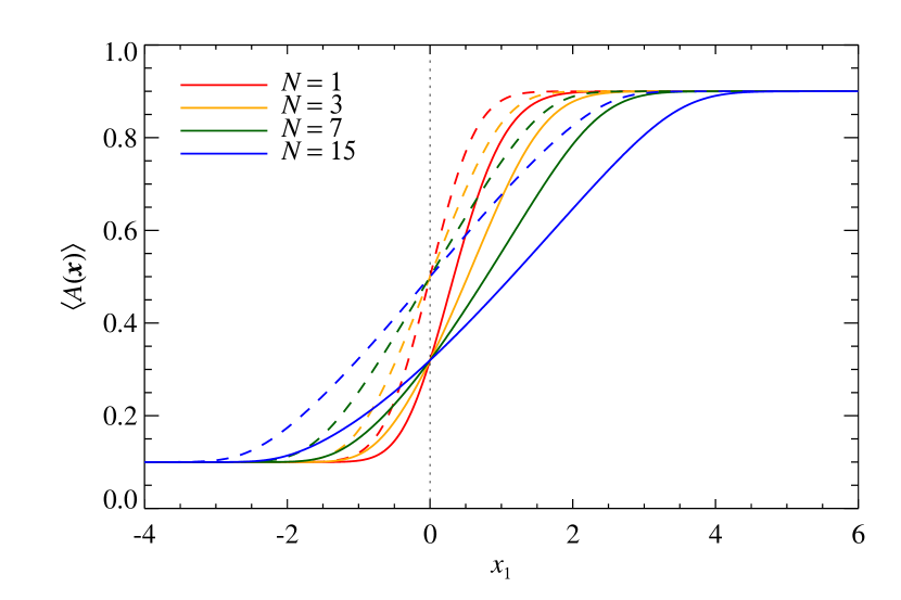
Figure 1: The bias of the nearest neighbors interpolation on a toy model where the true extinction is $A(\@vec{x})=0.1\mbox{ mag}$ for $x_{1}<0$ and $0.9\mbox{ mag}$ for $x_{1}\geq 0$. The solid lines show the average measured extinction of the nearest neighbours method, calculated using Eq. (9) for various number of neighbours $N$. The dashed lines show the extinction that one would measure if the density of stars were uniform on the whole field. Note that the solid lines are always below the dashed lines except at the extremes of this plot (where all estimators agree with the true value of $A$ there). For this plot we set $\alpha=0.34$, $k=1.55$, and $\rho_{0}=1$.

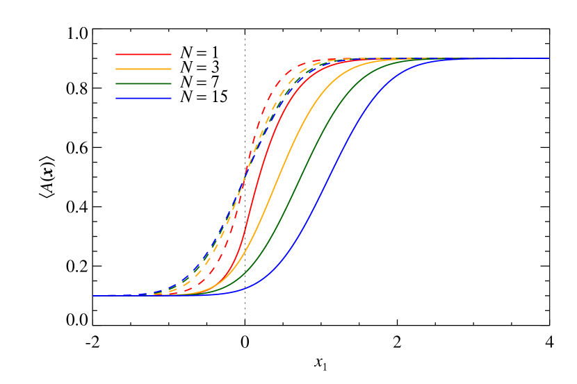
Figure 2: Similarly to Fig. 1, but for the median-nearest neighbors interpolation. Again, the solid lines, representing the expected mean measurements, are always below the dashed lines, representing the same measurements in the ideal case where the density of background stars is uniform within the whole field. Note that because of the properties of the median, for large values of $N$ the “transition” from $A=0.1\mbox{ mag}$ to $A=0.9\mbox{ mag}$ is faster than in Fig. 1.

The fact that $K(\@vec{x}^{\prime};\@vec{x})$ only depends on $\@vec{x}$ and $r=\lvert\@vec{x}-\@vec{x}^{\prime}\rvert$ (and not on the direction of the vector $\@vec{x}-\@vec{x}^{\prime}$) also implies that the nearest neighbors interpolation suffers from the bias discussed in this paper. Indeed, in the integral of Eq. (9) the kernel $K$ gives the same “weight” to all points on circles centered in $\@vec{x}$, irrespective of the specific value of $\rho$ on the various points of the circles (what matters here is only the average value of $\rho$ on a circle, and not the specific value on the various points). Hence, we do not expect that this technique can solve the bias introduced by the correlation between the extinction $A$ and the density of background stars $\rho$ expressed in Eq. (2), especially if steep gradients are present in the intrinsic cloud column density. We also expect that the bias present in the nearest neighbours interpolation increases with the number of neighbours $N$. Indeed, when $N$ increases, the “size” of the kernel $K(r;\@vec{x})$, i.e. the range in $r$ where the kernel is significantly different from 0, also increases because of the effects of the polynomial terms in Eq. (10). This, as shown by Eq. (9), implies that the kernel averages out more distant regions in the sky, where differences among the local densities can be significant.

In order to better understand the points mentioned in the previous paragraph, it is useful to look at simple example. Consider a cloud characterized by a Heaviside column density:

$$A(\@vec{x})=\begin{cases}A_{1}&\text{if $x_{1}<0\;,$}\\ A_{2}&\text{if $x_{1}\geq 0\;.$}\end{cases}$$ (14)

In this case we can basically carry out all the calculations analytically, and obtain for each value of $x_{1}$ the expected average measured extinction $\langle\hat{A}\rangle$. We do not report here the relevant equations, but rather show the results obtained in a typical case in Fig. 1. As shown by this plot, the nearest neighbours are clearly biased: for example, the various curves are not symmetric around $x_{1}=0$, and in addition

$$\langle\hat{A}\rangle=\frac{A_{1}10^{\alpha k_{\lambda}A_{1}}+A_{2}10^{\alpha k_{\lambda}A_{2}}}{10^{\alpha k_{\lambda}A_{1}}+10^{\alpha k_{\lambda}A_{2}}}<\frac{A_{1}+A_{2}}{2}\;.$$ (15)

In order to better understand the bias, we also plot in Fig. 1 the expected results in case of a uniform density, obtained assuming $\alpha=0$ in Eq. (2) (dashed lines): in this case the curves are perfectly symmetric around $x_{1}=0$ and $\langle\hat{A}\rangle=(A_{1}+A_{2})/2$. A comparison of the solid and dashed lines also confirms that curves with large $N$, being less steep, are biased on a larger interval around $x_{0}=0$. This is expected, since as shown by Eq. (10) the intrinsic size of the smoothing kernel $K$ increases with $N$.

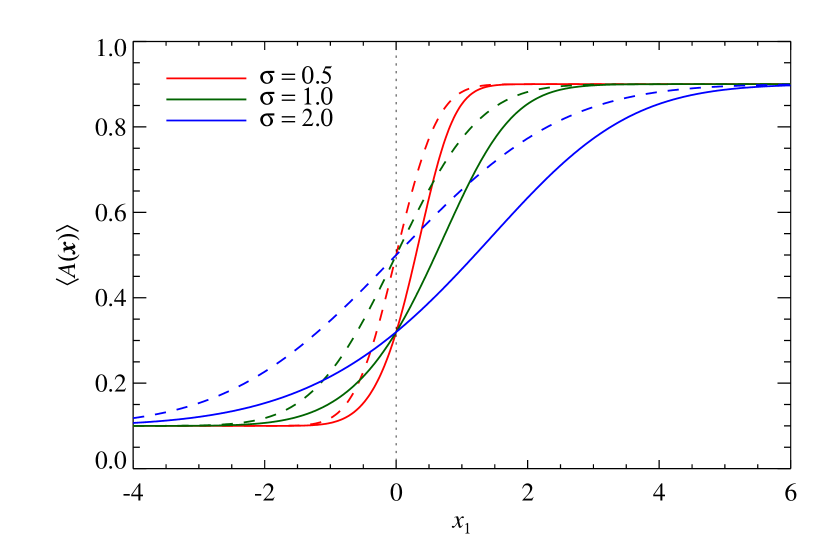
Figure 3: Similarly to Fig. 1, but for the moving average smoothing with a Gaussian window function with different dispersion parameters $\sigma$. As for Figs. 1 and 2, the solid lines, representing the expected mean measurements, are always below the dashed lines, representing the same measurements in the ideal case where the density of background stars is uniform within the whole field.

One might wanders if the bias decreases by using a median estimator instead of a simple mean, as done by Cambrésy et al. (2005, 2006). These authors still identify, for each sky position $\@vec{x}$, the $N$ nearest neighbour stars, and then evaluate a simple median of the relative extinction measurements. Luckily, it is possible to evaluate the exact statistical properties of the median estimator (see Lombardi, 2002, Appendix A). For this purpose, it is useful to evaluate the probability distribution $p_{N}(A;\@vec{x})$ that one of the $N$ neighbours around the position $\@vec{x}$ has a column density $A$:

$$p_{N}(A;\@vec{x})=\int\mathrm{d}\mu\,\mathrm{e}^{-\mu}\frac{\mu^{N-2}}{N!}\int_{B(\mu;\@vec{x})}\mathrm{d}x^{\prime}\,\rho(\@vec{x}^{\prime})\delta\bigl{(}A-A(\@vec{x})\bigr{)}\;,$$ (16)

where $B(\mu;\@vec{x})$ is the disk centered at $\@vec{x}$ and with radius $r$ defined by $\mu=\mu(r;\@vec{x})$ (note that since $\mu(r;\@vec{x})$, for $\@vec{x}$ fixed, is a monotonic function of $\@vec{x}^{\prime}$ this definition is unique). The cumulative distribution associated with $p_{N}(A;\@vec{x})$ is given by

$$P_{N}(A;\@vec{x})=\int\mathrm{d}\mu\,\mathrm{e}^{-\mu}\frac{\mu^{N-2}}{N!}\nu(\mu,A;\@vec{x})\;.$$ (17)

In this equation, $\nu(\mu,A;\@vec{x})$ is the integral of $\rho(\@vec{x})$ carried out over all points of $B(\mu;\@vec{x})$ where $A(\@vec{x}^{\prime})<A$:

$$\nu(\mu,A;\@vec{x})\equiv\int_{B(\mu;\@vec{x})\cap\{\@vec{x}^{\prime}|A(\@vec{x}^{\prime})<A\}}\rho(\@vec{x}^{\prime})\,\mathrm{d}x^{\prime}\;.$$ (18)

Note that $\nu(\mu,A;\@vec{x})\rightarrow\mu$ as $A\rightarrow\infty$. Finally, the median of the $N=2k-1$ nearest neighbours is then provided by the expression

$$p_{\mathrm{m}}(A)=k{N\choose k}p_{N}(A;\@vec{x})\bigl{[}P_{N}(A;\@vec{x})\bigr{]}^{k-1}\bigl{[}1-P_{N}(A;\@vec{x})\bigr{]}^{k-1}\;.$$ (19)

Although it is difficult to obtain a general expression for the bias introduced by the median-nearest neighbours estimator, it is clear that to first approximation the same arguments discussed above for the simple mean apply (note also that, trivially, when $N=1$ the two estimators are identical). However, for the simple example considered above, we can actually carry out the calculations using Eqs. (16–19) and show that the bias is still significant. Figure 2 summarizes the results obtained in the toy model described by Eq. (14), and proves that no real improvement is obtained from the use of a median estimator (cf. Fig. 1). In particular, a severe bias is still present, and its amount increases with $N$. For comparison, in Fig. 3 we also show the results obtained from the simple moving average smoothing discussed in Sect. 2.1: interestingly, the plot is very similar to the one for a the simple average nearest neighbors interpolation (Fig. 1). This, in reality, is not too much surprising because the expected average values $\bigl{\langle}A(x)\bigr{\rangle}$ measured with these two techniques can be described in terms of a simple convolution with some appropriate kernels [cf. Eq. (4) and (10); see also Lombardi, 2002].

In summary, a careful analysis of the nearest neighbors shows that this interpolation technique, for the specific case of extinction measurements, is still affected by a significant bias. At least for the case of a simple mean estimator, the origin of the problem can be traced to the different behaviour of the kernel $K(\@vec{x};\@vec{x}^{\prime})$ with respect to the density $\rho(\@vec{x}^{\prime})$ in Eq. (9): in particular, the kernel $K$ does not respond directly to variations of $\rho$, and instead depends only $\mu(\@vec{x}^{\prime};\@vec{x})$, i.e. on the total “mass” within a disk of radius $r=\langle\@vec{x}-\@vec{x}^{\prime}\rangle$.

3 Nicest: over-weighting high column-density measurements

As shown by Eq. (2.1), the bias discussed here strongly depends on the small-scale structure of the molecular cloud through the probability distribution $p_{A}(A)$. Although on large scales many models predict a log-normal distribution for $p_{A}$, clearly we should expect significant deviations from the theoretical expectations on the small scales often investigated in NIR studies. In addition, even at large scales the superposition of different cloud complexes, or a significant “thickness” of a cloud along the line of sight, can produce significant deviations from a log-normal distribution (Vázquez-Semadeni & García, 2001; see also Lombardi et al., 2006 for a case where the log-normal distribution is not a good approximation). Hence, we need to be able to correct for the substructure bias in a model independent way.

3.1 Statistical properties of the moving average smoothing

In order to better understand, and then fix, the bias present in Eq. (1) in the case of the moving average smoothing, we use the theory developed in Lombardi & Schneider (2001, 2002, 2003). The key equations to obtain the ensemble average of $\hat{A}(\@vec{x})$ are summarized below:

$$Q(s;\@vec{x})={} \int\bigl{[}\mathrm{e}^{-sw(\@vec{x}^{\prime};\@vec{x})}-1\bigr{]}\rho(\@vec{x}^{\prime})\,\mathrm{d}x^{\prime}$$ (20)

$$Y(s;\@vec{x})={} \exp\bigl{[}Q(s;\@vec{x})\bigr{]}\;,$$ (21)

$$C(w;\@vec{x})={} \frac{1}{1-P(x)}\int_{0}^{\infty}\mathrm{e}^{-ws}Y(s;\@vec{x})\,\mathrm{d}s\;,$$ (22)

$$\bigl{\langle}\hat{A}(\@vec{x})\bigr{\rangle}={} \int A(\@vec{x}^{\prime})w(\@vec{x}^{\prime};\@vec{x})C\bigl{(}w(\@vec{x}^{\prime};\@vec{x}),\@vec{x}\bigr{)}\rho(\@vec{x}^{\prime})\,\mathrm{d}x^{\prime}\;.$$ (23)

Let us briefly comment this set of equations:

• The equations are invariant upon the transformation $w(\@vec{x}^{\prime};\@vec{x})\mapsto qw(\@vec{x}^{\prime};\@vec{x})$, with $q$ positive constant. This is expected, since an overall multiplicative constant in the weight function does not effect Eq. (1). For simplicity, in the following we will assume, without loss of generality, that the weight function is normalized according to

  $$\int w(\@vec{x}^{\prime};\@vec{x})\rho(\@vec{x}^{\prime})\,\mathrm{d}x^{\prime}=1\;.$$ (24)

• The quantity $Q(s;\@vec{x})$ can be shown to be related to the Laplace transform of $p_{w}(w;\@vec{x})$, the probability distribution for the values of the weight function $w(\@vec{x}^{\prime};\@vec{x})$ with $\@vec{x}$ fixed.

• $P(\@vec{x})$ is the probability that no single star is present within the support $\pi_{w}(\@vec{x})$ of $w(\@vec{x}^{\prime};\@vec{x})$, defined as $\pi_{w}(\@vec{x})\equiv\{x^{\prime}\,|\,w(\@vec{x}^{\prime};\@vec{x})>0\}$. Hence, $P(\@vec{x})$ can be simply evaluated from

  $$P(\@vec{x})=\exp\left[-\int_{\pi_{w}(\@vec{x})}\rho(\@vec{x}^{\prime})\mathrm{d}x^{\prime}\right]\;.$$ (25)

  Note that $P(\@vec{x})=0$ for weight functions with infinite support (such as a Gaussian).

• $C(w;\@vec{x})$ is a simple Laplace transform of $Y(s;\@vec{x})$. This is the key quantity that enters the final result (23) together with the original smoothing function $w(\@vec{x}^{\prime};\@vec{x})$ and the star density $\rho(\@vec{x}^{\prime})$.

• A key parameter in the calculation of $C(w)$, and thus on the final result $\langle\hat{A}(\@vec{x})\rangle$, is the so-called weight number of objects $\mathcal{N}(\@vec{x})$, defined as

  $$\mathcal{N}(\@vec{x})\equiv\left[\bigl{[}1-P(\@vec{x})\bigr{]}\int\bigl{[}w(\@vec{x}^{\prime};\@vec{x})\bigr{]}^{2}\rho(\@vec{x}^{\prime})\,\mathrm{d}x^{\prime}\right]^{-1}\;,$$ (26)

  where as usual $w(\@vec{x}^{\prime};\@vec{x})$ is taken to be normalized according to Eq. (24). Informally, $\mathcal{N}(\@vec{x})$ counts the number of stars that contribute (with a weight significantly different from zero) to the average $\hat{A}(\@vec{x})$.

• In the limit $\mathcal{N}(\@vec{x})\gg 1$ it is possible to obtain a simple expression for $C(w;\@vec{x})$, which for $P(\@vec{x})=0$ takes the form

  $$C(w;\@vec{x})\simeq\frac{1}{1+w}+\frac{\bigl{[}\mathcal{N}(\@vec{x})\bigr{]}^{-1}}{(1+w)^{3}}\;.$$ (27)

  This expression shows that to lowest order $C\simeq 1-w+\mathcal{N}^{-1}$, where both terms $w$ and $\mathcal{N}^{-1}$ introduce a relative correction of order $\mathcal{N}^{-1}$ in the final result $\bigl{\langle}\hat{A}(\@vec{x})\bigr{\rangle}$.

The results summarized above rigorously prove the statements of Sect. 2.1. In particular, in the limit of a large weight number of objects $\mathcal{N}(\@vec{x})$, we have $C(w)\simeq 1$, and thus Eq. (23) together with the normalization (24) reduces to Eq. (4). In practice, numerical simulations show that Eq. (4) is already accurate for relatively small weight numbers (of the order of $\mathcal{N}\sim 10$; see Fig. 3 of Lombardi & Schneider, 2001).

3.2 A fix for the inhomogeneities bias

The bias of Eq. (1) is essentially due to a change in the density of extinction measurements as a function of $A$ [Eq. (2)]. In the framework of the moving average smoothing, it is thus reasonable to try to “compensate” this effect by including in the weights of the estimator (1) a factor $10^{\alpha k_{\lambda}A}$:

$$w_{n}=w(\@vec{x}_{n};\@vec{x})10^{\alpha k_{\lambda}\hat{A}_{n}}\;.$$ (28)

With this modification, we expect $\hat{A}$ to be unbiased provided that $\mathcal{N}$ is large (so that we can take $C\simeq 1$) and that measurement errors on $\hat{A}_{n}$ can be neglected. Instead, in presence of significant errors on the individual column density estimations, we expected $\hat{A}$ to be biased toward large extinctions. This happens because of the non-linearity of the introduced factor in $\hat{A}_{n}$: for example, $\hat{A}_{n}$ is symmetrically distributed around $A_{n}$, $10^{\alpha k_{\lambda}\hat{A}_{n}}\hat{A}_{n}$ will be skewed against values larger than $10^{\alpha k_{\lambda}A_{n}}A_{n}$. In summary, the modified weight of Eq. (28) removes (to a large degree) the bias due to the cloud substructure, but introduces a new bias related to the scatter of the individual extinction measurements. While the former is basically unpredictable, the latter can be estimated accurately provided we know the expected errors on $\hat{A}_{n}$.

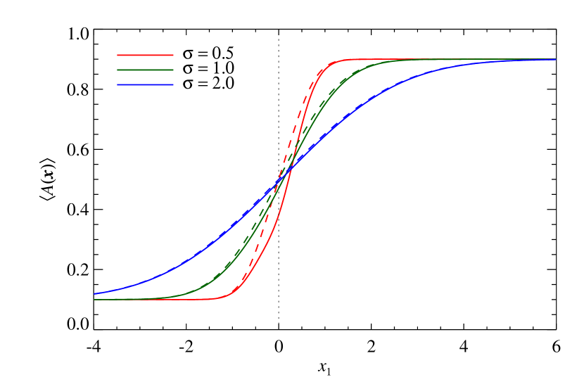
Figure 4: Similarly to Fig. 3, but for the Nicest moving average smoothing (see Sect. 3). In this case a significant bias is observed only for $\sigma=0.5$, which however correspond to a very small weight number $\mathcal{N}\simeq 2$.

In order to better understand the properties of the estimator (1) with the new weight, let us evaluate the average $\bigl{\langle}\hat{A}\bigr{\rangle}$. For simplicity, initially we will ignore measurement errors and focus on the effects introduced by a non-uniform density. We first note that Eq. (28) is equivalent to the use of a weight $w_{n}=w^{\prime}(\@vec{x}_{n};\@vec{x})$, where

$$w^{\prime}(\@vec{x}^{\prime};\@vec{x})\equiv w(\@vec{x}^{\prime};\@vec{x})/\rho(\@vec{x}^{\prime})\;.$$ (29)

We require the new weight $w^{\prime}(\@vec{x}^{\prime};\@vec{x})$ to be normalized according to Eq. (24), which implies

$$\int w(\@vec{x}^{\prime};\@vec{x})\,\mathrm{d}x^{\prime}=1\;.$$ (30)

Interestingly, the normalization condition (30) for $w$ does not depend on the density $\rho$ anymore, and it is thus possible to choose for $w$ a spatially invariant function $w(\@vec{x}^{\prime};\@vec{x})=w(\@vec{x}^{\prime}-\@vec{x})$ (a typical choice would be a Gaussian, $w\propto\mathrm{e}^{-|\@vec{x}^{\prime}-\@vec{x}|/2\sigma^{2}}$). We have then

$$\bigl{\langle}\hat{A}(\@vec{x})\bigr{\rangle}={} \int A(\@vec{x}^{\prime})w^{\prime}(\@vec{x}^{\prime};\@vec{x})\bigl{[}1-w^{\prime}(\@vec{x}^{\prime};\@vec{x})+\mathcal{N}^{-1}(\@vec{x})\bigr{]}\rho(\@vec{x}^{\prime})\,\mathrm{d}x^{\prime}$$

$${}={} \int A(\@vec{x}^{\prime})w(\@vec{x}^{\prime};\@vec{x})\bigl{[}1-w(\@vec{x}^{\prime};\@vec{x})/\rho(\@vec{x}^{\prime})+\mathcal{N}^{-1}(\@vec{x})\bigr{]}\,\mathrm{d}x^{\prime}\;.$$ (31)

After a few manipulations we can rewrite this expression in the form

$$\bigl{\langle}\hat{A}(\@vec{x})\bigr{\rangle}={} \bar{A}(\@vec{x})-\frac{1}{\rho_{0}}\int w^{2}(\@vec{x}^{\prime};\@vec{x})10^{\alpha k_{\lambda}A(\@vec{x}^{\prime})}\bigl{[}A(\@vec{x}^{\prime})-\bar{A}(\@vec{x})\bigr{]}\,\mathrm{d}x^{\prime}$$

$${}\simeq{} \bar{A}(\@vec{x})-\frac{10^{\alpha k_{\lambda}\bar{A}(\@vec{x})}}{\rho_{0}}\int w^{2}(\@vec{x}^{\prime};\@vec{x})\bigl{[}\Delta(\@vec{x}^{\prime};\@vec{x})$$

$$\phantom{\bar{A}(\@vec{x})-\frac{10^{\alpha k_{\lambda}\bar{A}(\@vec{x})}}{\rho_{0}}\int w^{2}(\@vec{x}^{\prime};\@vec{x})\bigl{[}}+\beta\Delta^{2}(\@vec{x}^{\prime};\@vec{x})\bigr{]}\,\mathrm{d}x\;,$$ (32)

where in the second equality we have expanded the exponential term to first order using the definitions following Eq. (2.1). In summary, the bias $\bigl{\langle}\hat{A}(\@vec{x})\bigr{\rangle}-\bar{A}(\@vec{x})$ of the proposed estimator is composed of two terms:

• A weighted average of $\Delta(\@vec{x}^{\prime};\@vec{x})$. Since the weighted average uses $w^{2}(\@vec{x}^{\prime};\@vec{x})$ as weight, this term is not expected to vanish identically unless the weight is a top-hat function [cf. Eq. (2.1), where instead the weighted average involves $w(\@vec{x}^{\prime};\@vec{x})$ and therefore no linear contribution in $\Delta$ is present]. Still, we do not expect any systematic bias related to this term, because on average $\Delta(\@vec{x}^{\prime};\@vec{x})$ by construction has alternating sign.

• A weighted average of $\Delta^{2}(\@vec{x}^{\prime};\@vec{x})$. This term is manifestly negative and therefore introduces a bias in the result. The bias is very similar to the original bias discussed in Eq. (2.1): it is proportional to $\beta\equiv\alpha k_{\lambda}\ln 10$, and depends on the scatter $\Delta(\@vec{x}^{\prime};\@vec{x})\equiv A(\@vec{x}^{\prime})-\bar{A}(\@vec{x})$ of the local column density with respect to its average value. However, there is a significant difference: the bias is inversely proportional to $\rho_{0}10^{-\alpha k_{\lambda}\bar{A}(\@vec{x})}$, i.e. to the local average density within the weight function; moreover, the average is taken over $w^{2}$ instead of $w$. These two differences, together, indicate that the bias of Eq. (3.2), compared to the on of Eq. (2.1), is smaller by a factor $\sim\mathcal{N}(\@vec{x})$.

In other words, the modification of the weight operated by Eq. (28) reduces the bias present in the original simple moving weight average by a factor $\mathcal{N}(\@vec{x})$, which in typical cases is significantly larger than unity. On the other hand, the fact that the method is ineffective then $\mathcal{N}$ is low is evident from the definition of $w_{n}$: in particular, as $\rho\rightarrow 0$ we expect that only a single star contributes to the averages of Eq. (1) with a weight $w_{n}=w(\@vec{x}_{n};x)10^{\alpha k_{\lambda}\hat{A}_{n}}$ significantly different from zero, but then trivially $\hat{A}=\hat{A}_{n}$ and no correction is effectively performed.

In Fig. 4 we show the effects of the proposed smoothing technique on the toy-model discussed in Sect. 2.2. A comparison with Fig. 3 shows that the Nicer interpolation is very effective in reducing the bias of the simple moving average interpolation, especially for relatively large values of the smoothing factor $\sigma$ (and thus of the weight number of objects $\mathcal{N}$).

We now consider the effects of measurement errors in the modified estimator. For simplicity, we consider the limit of a large number of stars ($\mathcal{N}\gg 1$), so that $C(w)\simeq 1$ (in any case, as shown above, the technique proposed is inefficient when $\mathcal{N}$ is of order of unity). In this case, a simple calculation shows that measurements errors introduce a bias $B_{\mathrm{err}}$ of the order

$$B_{\mathrm{err}}\simeq\beta\frac{\sum_{n}w_{n}\sigma_{n}^{2}}{\sum_{n}w_{n}}\;,$$ (33)

where $\{\sigma^{2}_{n}\}$ are the variances on $\{\hat{A}_{n}\}$. In other words, the method proposed in this paper introduces a small bias toward large extinction values. In order to estimate the order of magnitude of $B_{\mathrm{err}}$, we note that the median error in $K$ band extinctions on Nicer column density estimates from the 2MASS catalog is typically $\sigma\simeq 0.13\mbox{ mag}$, and that less than $1\%$ of stars have $\sigma>0.2\mbox{ mag}$. Taking $\sigma_{n}=0.13\mbox{ mag}$ for all stars in Eq. (33), we find a bias $\langle\hat{A}\rangle-A\simeq 0.02\mbox{ mag}$ (always in the $K$ band). Interestingly, although very small this bias, in contrast to the one described by Eq. (3.2), can be corrected to first order because its expression involves only known quantities.

In summary, we propose to replace the estimator (1) with

$$\boxed{\hat{A}=\frac{\sum_{n}w_{n}\hat{A}_{n}}{\sum_{n}w_{n}}-\beta\,\frac{\sum_{n}w_{n}\sigma^{2}_{n}}{\sum_{n}w_{n}}\;,}$$ (34)

where $w_{n}\equiv w(\@vec{x}^{\prime};\@vec{x})10^{\alpha k_{\lambda}\hat{A}_{n}}$. This new estimator, that we name Nicest, significantly reduces the bias due small-scale inhomogeneities in the extinction map and is (to first order) unbiased with respect to uncertainties on $\hat{A}_{n}$.

If one is ready to accept a small bias on $\hat{A}$ for extinction measurement uncertainties, it is also possible to use Eq. (34) without the last term. In this respect, we also note that the correcting factor present in Eq. (34) is independent of the local extinction, and only depends on the individual errors on the measurements (these typically are a combination of the photometric uncertainties and of the intrinsic scatter of colors of the stellar population considered). As a result, it is not unrealistic to expect that this factor is approximately constant within the field of observation, and that it is equally present in the control field used to fix the zero of the extinction.

Finally, we note that in Nicest a central role is played by the slope of the number counts $\alpha$, operationally defined through Eq. (2). In reality, however, it clear that Eq. (2) cannot strictly hold, because there is an upper limit on the (un-reddened) magnitude of stars. Hence, depending on the limiting magnitude of the observations, there is an upper limit to the measurable extinction of stars. As a result, in regions where the extinction is larger than this limit, the density of background stars vanishes, with the result that in these cases even Nicest cannot be unbiased. The exact value of the upper measurable extinction depends on many factors, including the waveband $\lambda$ and limiting magnitude $m_{\mathrm{max}}$ of the observations, and the distance $d$ of the molecular cloud. An approximate relation for the maximum extinction $A_{\mathrm{max}}$ is

$$A_{\mathrm{max}}\sim\frac{1}{k_{\lambda}}\left[m_{\mathrm{max}}-M_{\mathrm{max}}-5\log_{10}\left(\frac{d}{10\mbox{ pc}}\right)\right]\;,$$ (35)

where $M_{\mathrm{max}}$ is the maximum absolute magnitude of stars in the band considered. The maximum extinction $A_{\mathrm{max}}$ should be evaluated in each specific case; for example, for typical 2MASS observations, using $m_{\mathrm{max}}\simeq 15\mbox{ mag}$, $k_{H}=1.55$ (Indebetouw et al., 2005), and $M_{\mathrm{max}}\simeq-5\mbox{ mag}$ we obtain $A_{\mathrm{max}}\simeq 10\mbox{ mag}$ for a cloud located at $100\mbox{ pc}$.

3.3 Foreground stars

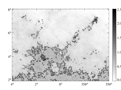
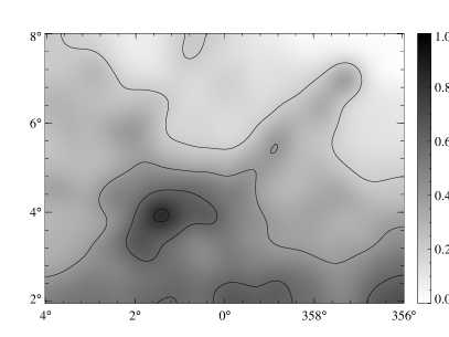
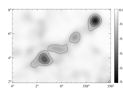
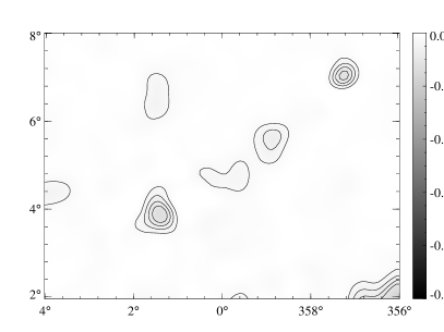
Figure 5: Top left. The original 2MASS/Nicer map of the Pipe nebula used in the simulations. Top right. The mean reconstructed map that one would obtain if the density of background star were uniform. This is basically a smoothed version of the original map in the left. Levels are spaced at $0.2\mbox{ mag}$. Bottom left. The difference between the average reconstructed maps, calculated from background stars following the density of Eq. (2), and the average map at top right. Levels are spaced at $0.02\mbox{ mag}$. Bottom right. Same map as bottom left, but using the improved method presented in this paper. Levels are spaced at $0.0025\mbox{ mag}$.

Foreground stars do not contribute to the extinction signal, but do contribute to the noise of the estimators (1) and (34), and thus whenever possible they should be excluded from the analysis. Usually, foreground stars are easily identified in high ($A_{K}>1\mbox{ mag}$) column density regions, but are almost impossible to distinguish in low and mid extinction regions. So far we assumed that all stars are background to the cloud, but clearly in real observations we should expect a fraction $f$ of foreground objects. In principle, if this fraction is known, we could correct the column density estimate $\hat{A}$ into $\hat{A}/(1-f)$: in this way, we would obtain an unbiased estimator of the column density at the price of an increased noise (due to foreground objects). In practice, the fraction of foreground stars is itself an increasing function of the local column density, i.e. $f=f(A)$, because of the decreased density of background stars in highly extincted regions. Hence, the simple scheme proposed above is not easily implemented.

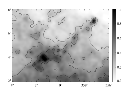
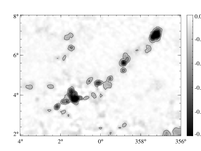
Figure 6: Left. Average reconstructed map using a 1-star ($N=1$) Voronoi method, assuming a uniform distribution of stars. Levels are spaced at $0.2\mbox{ mag}$. Right. Difference between the average reconstructed Voronoi map, obtained from background stars following the density of Eq. (2), and the average true map to the left. Levels are spaced at $0.02\mbox{ mag}$

Interestingly, Nicest perfectly adapts to the presence of foreground stars. Suppose that in regions with negligible extinction a fraction $f_{0}\equiv f(A=0)<1$ of stars is foreground to the cloud: then, in our notation, we can rephrase this by assigning a non-vanishing probability to $p_{A}(A=0)$, i.e. by treating foreground stars as a special case of substructure (much like “holes” in the cloud). As we consider higher density regions, the fraction $f(A)$ of foreground stars increases but, because of the correcting factor in $w_{n}$, we still expect to measure $(1-f_{0})A$: in other words, the estimator $\hat{A}/(1-f_{0})$, with $\hat{A}$ given by Eq. (34) is expected to be unbiased both for small-scale inhomogeneities and for foreground contamination. Note that correcting factor $(1-f_{0})^{-1}$ is usually very close to $1$ for nearby molecular clouds, and can be easily evaluated by comparing the density of foreground stars (easily measured in highly extincted regions) with the total density of stars in regions free from extinction.

4 Simulations

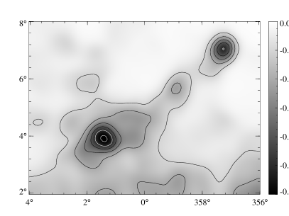
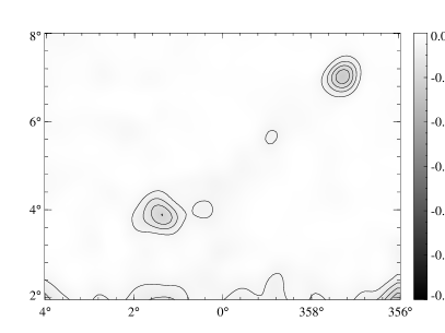
Figure 7: Same as Fig. 5 (bottom), but with a fraction of $f=0.05$ of foreground stars. The increases of relative number of foreground stars in the denser regions of the cloud makes the bias more pronounced. Still, Nicest performs very well. Contours levels are spaced at $0.02\mbox{ mag}$ in the Nicer plot (left) and at $0.005\mbox{ mag}$ in the Nicest plot (right); contours at $-0.1\mbox{ mag}$ or below are plotted in white.

In order to test the effects of substructures and the reliability of the method proposed here in a real case scenario we performed a series of simulations. We started from a 2MASS/Nicer map of the Pipe nebula (Lombardi et al., 2006), a nearby complex of molecular clouds seen in projection to the Galactic bulge, an ideal case for extinction studies (see also Alves et al., 2008; Onishi et al., 1999). We took this map as the true dust column density of a cloud complex, and simulated a set of background stars. In order to show the effects of substructures, we used a very small density of background stars ($25\mbox{ stars deg}^{-2}$ instead of the original $\sim 9.4\times 10^{5}\mbox{ stars deg}^{-2}$ used to build the 2MASS/Nicer map). This, effectively, correspond to a linear downsize of the structures of the Pipe nebula by a factor $\sim 60$.

The simulations were carried out using the following simple technique. We generated a set of background stars uniformly distributed on the field of view. The stars were characterized by exponential number counts with exponent $\alpha=0.34$ in the $K$ band and by intrinsic color and color scatters similar to the ones observed in the 2MASS catalog (see Table 2 of Lombardi, 2005 for a complete list of the parameters used). We added to each star magnitude the local value of the of the 2MASS/Nicer extinction and also some random measurement errors:

$$\hat{J}_{n}={} J_{n}+k_{K}A_{K}(\@vec{x}_{n})+\varepsilon^{(J)}_{n}\;,$$ (36)

$$\hat{H}_{n}={} H_{n}+k_{H}A_{K}(\@vec{x}_{n})+\varepsilon^{(H)}_{n}\;,$$ (37)

$$\hat{K}_{n}={} K+A_{k}(\@vec{x}_{n})+\varepsilon^{(K)}_{n}\;,$$ (38)

where $\varepsilon^{(J,H,K)}_{n}$ denote random variables used to model the photometric errors of the stars, and where as usual we used the hat to denote measured quantities. For simplicity, here, we took the errors as normal distributed random variables with constant variance $0.05\mbox{ mag}$ in all bands (the typical median variance of 2MASS magnitudes); moreover, we assumed a hard completeness limit at $15\mbox{ mag}$ in all bands (i.e., if a magnitude exceeded $15$ we took the star as not detected in the corresponding band). We then applied the Nicer algorithm to these data, thus obtaining, for each star, its measured extinction and related error. Finally, we produced smooth extinction maps by interpolating the individual extinction measurements with three different techniques: (1) simple moving average using Eq. (1); (2) modified moving average using Nicest [Eq. (34)]; (3) nearest neighbour interpolation with a single star ($N=1$).

We repeated the whole procedure $1\,000$ times, using each time a different set of random background stars, and took the average maps $\hat{A}(\@vec{x})$ obtained with the three techniques. We then compared these average maps with similar maps obtained from uniformly distributed stars (in order to produce such maps, we applied the completeness limit to un-extincted magnitudes). Figures 5 and 6 show the results obtained, which are in clear favour of Nicest. In particular, both the simple moving average and the nearest neighbor suffer from significant biases, up to $A_{K}\simeq 0.1\mbox{ mag}$ or above, particularly in the most dense regions of the Pipe nebula. As shown in various papers (e.g. Lada et al., 1994; Lombardi et al., 2006, 2008), the amount of small scale structure present in dark molecular clouds increases with the column density, and thus it is not surprising that the larger biases are observed there. In contrast, the method presented in this paper reduces the bias by $\sim 10$, a factor comparable to the weight number of stars $\mathcal{N}$ (which in our simulations is $\mathcal{N}\simeq 10$ in the higher column density regions).

The simulation performed here allows us to evaluate also the average quadratic difference between the extinction map obtained for the various methods $\hat{A}(\@vec{x})$ and the true (smoothed) map $\bar{A}(\@vec{x})$, i.e. the quantity

$$\bigl{\langle}\bigl{[}\hat{A}(\@vec{x})-\bar{A}(\@vec{x})\bigr{]}^{2}\bigr{\rangle}=\mathrm{Var}\bigl{[}\hat{A}(\@vec{x})\bigr{]}+\bigl{[}\bigl{\langle}\hat{A}(\@vec{x})-\bar{A}(\@vec{x})x\bigr{\rangle}\bigr{]}^{2}\;.$$ (39)

As shown by the above equation, the quantity considered here can be written as the sum of the variance and the square of the bias of the extinction map. Our simulations show that, although Nicest, as expected, has a slightly larger variance then Nicer, there is still a gain by a factor at least two in the squared difference of Eq. (39). In other words, the significant reduction in the bias performed by Nicest largely compensate the increase in the scatter introduced by this method. A naive comparison between the results obtained from Nicest and from the Voronoi method would provide even larger differences in favour of Nicest, but we stress that since the Voronoi method interpolates the extinctions over a fixed number of stars (typically smaller than the one employed by Nicest in our simulations) a direct comparison is not possible.

Figure 7 shows the result of simulation carried out with the presence of foreground stars. In particular, we generated stars following the same prescriptions described in the previous paragraph, but allowing for a fraction $f_{0}=0.05$ of foreground objects. Because of the effects of extinction, the effective fraction of foreground objects increases in the most dense regions of the cloud, which usually are also the ones with the larger substructures: the two biases thus add up and can be particularly severe. As shown by Fig. 7, Nicest is effectively able to cope with relatively large fractions of foreground stars while still providing a virtually unbiased column density estimate.

5 A sample application

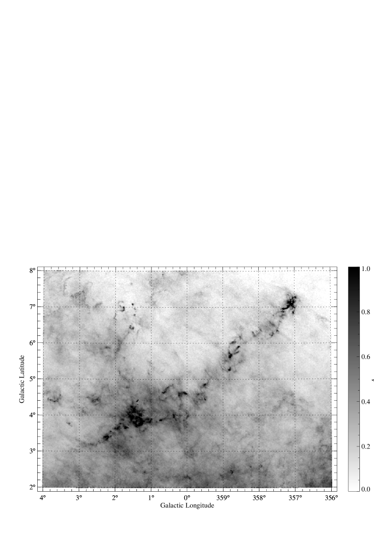
Figure 8: The Nicest extinction map of the Pipe nebula, using the modified estimator (28).

The method presented in this paper was finally applied to the whole 2MASS point source catalog for the Pipe nebula region. We used the 4.5 million stars of the 2MASS catalog located in the window

$$-4^{\circ}<{} l<4^{\circ}\;, +2^{\circ}<{} b<+8^{\circ}\;.$$ (40)

The analysis was carried out following the prescriptions of Lombardi & Alves (2001), but using the modified estimator (34) to evaluate $\hat{A}$. In particular, we generated the final extinction map, shown in Fig. 8, on a grid of about $1000\times 750$ points, with scale $30\mbox{ arcsec}$ per pixel, and with Gaussian smoothing characterized by $\mbox{FWHM}=1\mbox{ arcmin}$. The slope of the number counts was estimated to be $\alpha=0.32\pm 0.02$ in the $H$ band.

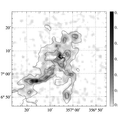
Figure 9: The difference between the modified extinction estimates [Eq. (28)] and the standard ones [Eq. (1)] around Barnard 59. The contour levels are at $A=\{0.5,1.0,1.5,2.0\}\mbox{ mag}$ of the map of Fig. 8.

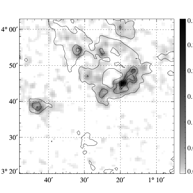
Figure 10: The difference between the modified extinction estimates [Eq. (28)] and the standard ones [Eq. (1)] around the peak ID 3 of Lombardi et al. (2006). The contour levels are at $A=\{0.5,1.0,1.5,2.0\}\mbox{ mag}$ of the map of Fig. 8.

The final, effective density of stars of about $8$ stars per pixel guarantees that the approximation used to derive the unbiased estimator (34) is valid, and that a significant improvement over the standard Nicer method can be expected. The largest extinction was measured close to Barnard 59, where $\hat{A}\simeq 2.68\mbox{ mag}$ (a value that is $0.41\mbox{ mag}$ larger than what obtained in (Lombardi et al., 2006)).

Figures 9 and 10 show a comparison between dense regions mapped using Nicer and Nicest. We note that, as expected, the two methods are equivalent in low-density regions, while the new one consistently estimates larger column densities as $A$ increases. The same effect can be appreciated more quantitatively from Fig. 11, where we plot the relationship between the average estimates $\hat{A}$ obtained in Lombardi et al. (2006) and here.

Figure 11: The average difference $\Delta A$ between the estimators (28) and (1) as a function of the estimated column density $A$. The lower, solid line is relative to the Pipe nebula map at $\mbox{FWHM}=1\mbox{ arcmin}$ resolution; the upper dashed line is at for a resolution $\mbox{FWHM}=1.5\mbox{ arcmin}$. The latter plot is essentially what we would obtain at a $\mbox{FWHM}=1\mbox{ arcmin}$ if the distance of the Pipe nebula increases by a factor $1.5$.

Finally, we argue that the plot of Fig. 11 is strongly related to Fig. 9 of Lombardi et al. (2006) where we show the increase in the scatter of $\hat{A}_{n}$ for the different stars used in each point of the extinction map as a function of the average $\hat{A}$ in the point. This $A$-$\sigma$ relation is most likely due to unresolved substructures in the cloud, that are expected to be more prominent in high-density regions. Recently, we reconsidered the $A$-$\sigma$ relation and defined a quantity called $\Delta^{2}(\@vec{x})$ (Lombardi et al., 2008). This quantity is simply related to the local scatter of measured extinctions, but also properly takes into account the contribution of measurement errors to the observed scatter. Interestingly, this quantity can be defined in terms of simple observables, and can be shown to be directly related to the local scatter of column densities:

$$\Delta^{2}(\@vec{x})=\frac{\sum_{n}w_{n}\Delta_{n}^{2}}{\sum_{n}w_{n}}\;,$$ (41)

where $\Delta_{n}\equiv A(\@vec{x}_{n})-\bar{A}(\@vec{x})$ is the difference between the column extinction at the position of the $n$-th star and the local average column extinction. A comparison of Eq. (41) with Eq. (2.1) clearly shows that, except for a numerical factor $\beta$, the bias expected in the standard Nicer method is simply proportional to the $\Delta^{2}(\@vec{x})$ of (Lombardi et al., 2008).

6 Discussion

The numerical simulations and a first sample application of Nicest have shown that the method presented in this paper can significantly alleviate the bias introduced by small-scale structures and by foreground stars in extinction studies. Of course, Nicest too has some limitations, which however are largely unavoidable (and thus inherent to any extinction-based method).

First, we note that in order for Nicest to work effectively, the weight number of background stars $\mathcal{N}$ must be significantly larger than unity: as shown in Sect. 3.2, $\mathcal{N}$ is directly related to the reduction in the bias provided by Nicest with respect to Nicer, and thus having $\mathcal{N}\sim 1$ does not give any benefit. This point is also important when correcting for foreground star contamination. For example, if $\mathcal{N}\sim 1$ and the local fraction $f$ of foreground stars is large (e.g., because we are in a particularly dense core), on average we do not expect any background star, and we will thus consistently measure a vanishing extinction. Hence, Nicest, like any other extinction based method, only works if there are a sizable number of background stars that can be used for reliable extinction measurements.

The above point might be interpreted as an exceedingly stringent requirement for the smoothing window used in Nicest. In fact, if a weight function $w(\@vec{x}^{\prime};\@vec{x})=w(\@vec{x}^{\prime}-\@vec{x})$ invariant upon translation is used, this function should be taken broad enough to guarantee that the weight number of background stars $\mathcal{N}(\@vec{x})$ is significantly larger than unit everywhere. This, in turn, would imply that $\mathcal{N}\gg 1$ in the intermediate extinction regions, i.e. that the extinction map in these regions has a poor resolution, well below the limits imposed by the density of background stars. In reality, the whole derivation of the statistical properties of the Nicest technique is still valid for weight functions which are not spatially invariant. Hence, one does not need to use a fixed window size for $w(\@vec{x}^{\prime};\@vec{x})$, but rather this function could be taken to change shape for different locations $\@vec{x}$. For example, a simple scheme could be the use of a Gaussian shape for $w(\@vec{x}^{\prime};\@vec{x})$ with the typical scale chosen according to a local estimate of the density of background stars, in a way such that $\mathcal{N}(\@vec{x})\sim\mbox{const}\sim 10$. This choice would guarantee an optimal resolution everywhere, and would still allow one to make use of the Nicer technique to reduce the inhomogeneity bias.

Another point to keep in mind is that Nicest gives a large weight to red sources. This has two potential unwanted consequences. First, it introduces a small bias, that has been corrected to first order in Eq. (34). Second, as shown also by the numerical simulations described in Sect. 5, it slightly increases the noise in the final map. Again, since the noise in final map $\hat{A}(\@vec{x})$ is proportional to $1/\mathcal{N}$, the solution is to make sure that $\mathcal{N}$ is sufficiently large. We believe that a small increase in the noise is a fair price to pay for the significant reduction in the bias provided by Nicest over Nicer (see also Eadie et al., 1971).

A potentially more severe problem can be young stellar objects (YSOs) with infrared excess. These sources can be present in the most dense star-forming cores of molecular clouds, where they can severely bias our method. We note, however, that since these sources have peculiar colors and are not usually present in the control field used for the calibration, they represent anyway a problem for all extinction based methods, including Nicer and the nearest neighbours ones. A median estimator is in principle safer to use in these cases, as long as the YSOs present in the core are a minority of the total number of background stars observed in the region; unfortunately, the tendency of YSOs to appear in clusters does not help here (note also that a median is usually more noisy than the simple average). In any case, the obvious solution is thus to exclude as much as possible YSOs from the list of sources used in the extinction maps.

Finally, let us briefly mention alternative possibilities to reduce the bias considered in this paper. Since the substructure bias is due to a relationship between the local density $\rho(\@vec{x})$ and the extinction map $A(\@vec{x})$ [Eq. (2)], one could try to use a tracer of the local density to perform the correction. We discussed already a method based on this concept, the nearest neighbours interpolation. However, as shown in Sect. 4, this method fails (see also Sect. 2.2). In general, a problem with methods based on the local estimate of the density of background stars is that one needs to be able to obtain $\rho(\@vec{x})$ on scales smaller than the ones that characterize the weight $w(\@vec{x}^{\prime};\@vec{x})$, or otherwise it is not possible to give different weights to the different stars that contribute significantly to the weighted average of Eq. (1). However, if the density of background stars is large enough to have a good handle on the local density $\rho(\@vec{x})$, one basically does not need to care about substructures, because it is always possible to make extinction maps at the same resolution as the density map. Hence, the only effective way to deal with substructures involves a use of the local extinction measurements, as done in Nicest. Note also that any density-based correction will be completely ineffective with foreground stars, in contrast to the method presented here.

7 Conclusions

The main results obtained in this paper can be summarized in the following points:

• We discussed the effects of small scale inhomogeneities in the NIR extinction maps based on color excess methods, and showed that large inhomogeneities can significantly bias standard extinction maps toward low column densities.

• We proposed a new estimator for $\hat{A}$, Nicest, and we showed that it is (i) equivalent to the usual estimator in low-density regions, (ii) unbiased and robust for any value of $A$, i.e. insensitive to the actual form and amount of substructure present in the cloud.

• We showed that the new estimator is also suitable in presence contamination by foreground stars.

• We tested Nicest against numerical simulations, and showed that it effectively reduces by a large factor the biases due to substructures and to foreground stars. We also tested an alternative approach, the nearest neighbor, and showed that the results obtained from this interpolation are still severely biased.

• We applied Nicest to the Pipe nebula and showed a few preliminary properties of the resulting extinction map. We also noted a direct connection between the bias of the Nicer and the $\Delta^{2}$ map defined by (Lombardi et al., 2008).