A record-driven growth process

Abstract

We introduce a novel stochastic growth process, the Record-driven growth process, which originates from the analysis of a class of growing networks in a universal limiting regime. Nodes are added one by one to a network, each node possessing a quality. The new incoming node connects to the preexisting node with best quality, that is, with record value for the quality. The emergent structure is that of a growing network, where groups are formed around record nodes (nodes endowed with the best intrinsic qualities). Special emphasis is put on the statistics of leaders (nodes whose degrees are the largest). The asymptotic probability for a node to be a leader is equal to the Golomb-Dickman constant $\omega=0.624\,329\dots$, which arises in problems of combinatorical nature. This outcome solves the problem of the determination of the record breaking rate for the sequence of correlated inter-record intervals. The process exhibits temporal self-similarity in the late-time regime. Connections with the statistics of the cycles of random permutations, the statistical properties of randomly broken intervals, and the Kesten variable are given.

,

1 Introduction

In the present work we introduce and study a novel stochastic growth process, the Record-driven (RD) growth process, which originates from the analysis of a class of growing networks in a universal limiting regime. As we shall see, this process is also related to three other fields, namely the statistics of the cycles of random permutations, the statistical properties of randomly broken intervals, and the Kesten variable.

The RD growth process originates from a class of growing networks with a preferential attachment rule, amongst which the most well known representative is the model of Barabási and Albert (BA) [1]. The latter provides a natural explanation for the main features observed in real networks [2, 3, 4, 5], and chiefly their scale-freeness, testified by the power-law fall-off of their degree distribution. Relevant for our purpose are networks where the attachment rule involves both the degree of the nodes and their intrinsic quality or fitness, an extension of the original BA model which is due to Bianconi and Barabási (BB) [6]. The BB model has the remarkable feature that it exhibits a continuous condensation transition, analogous to the Bose-Einstein condensation.

A general definition of this class of networks is as follows. The network being initially empty, at each integer time step, $n=1,2,\dots$, a new node, labeled by its birth date $n$, is added. Node $n$ is endowed once and for all with an intrinsic quality $\eta_{n}$, modeled by a quenched random variable drawn from some given distribution. This node (except for the first one) connects by one link to any of the earlier nodes ($i=1,\dots,n-1$) with probability

$$p_{i,n}=\frac{\eta_{i}\,h(k_{i})}{Z_{n-1}},$$ (1.1)

where $h(k_{i})$ is a function of the degree $k_{i}$ of node $i$, i.e., the number of nodes already connected to node $i$ at time $n-1$. The denominator

$$Z_{n-1}=\sum_{i=1}^{n-1}\eta_{i}\,h(k_{i})$$ (1.2)

is a normalization factor. The probability $p_{i,n}$ is thus proportional to an intrinsic factor, the quality $\eta_{i}$ of node $i$, and to a dynamical one, represented by $h(k_{i})$. Preferential attachment to nodes whose degree is already larger is realized whenever the function $h(k_{i})$ is an increasing function of the degree $k_{i}$. Finally, temperature $T$ is introduced into the model by considering the qualities as activated variables, i.e., by setting

$$\eta_{n}=\exp(-\varepsilon_{n}/T),$$ (1.3)

and assuming that the activation energies $\varepsilon_{n}$ are drawn from a given temperature-independent continuous distribution.

The BA and BB models in their original forms both correspond to the linear function $h(k)=k$. The BA model corresponds to the limiting case of infinite temperature.

After time step $n$ is completed the network consists of $n$ nodes connected by $n-1$ links. It therefore has the topology of a tree. In the rest of the paper we use a slightly modified definition of the degree, keeping abusively the same notation, $k_{i}$. We define the degree of a given node as the number of incoming links on this node, taking aside its unique outgoing link, except for the first node, which has no outgoing link. This new definition corresponds to shifting by one unit the former quantity, $k_{i}\to k_{i}-1$, except for the first node. The degrees thus defined sum up to the number of links, i.e.,

$$\sum_{i=1}^{n}k_{i}=n-1.$$ (1.4)

As we now explain, the RD growth process is the zero-temperature limit of the class of models described above. In this limit, at any time $n$ the node $i$ with the lowest energy:

$$\varepsilon_{i}=\min(\varepsilon_{1},\dots,\varepsilon_{n-1}),$$ (1.5)

i.e., with the highest quality, has an attachment probability $p_{i,n}$ which is overwhelmingly larger than all the other ones, since the ratio $p_{i,n}/p_{j,n}$ grows exponentially at low temperature, as $\exp((\varepsilon_{j}-\varepsilon_{i})/T)$. Every new node $n$ therefore connects to the earlier node $i$ with best quality at time $n$, given by (1.5). The successive best qualities are known as records [7, 8, 9, 10]. The corresponding nodes, that we term record nodes, are therefore the only ones whose degree grows. This process is universal in a very strong sense. It is independent of the function $h(k)$ and of the distribution of the node energies, provided the latter is continuous, so that the event $\varepsilon_{i}=\varepsilon_{j}$ with $i\neq j$ has zero probability. In particular, the RD growth process is independent of whether the model has a condensation transition or not.

Let us summarize the definition of the process and give a pictorial interpretation of it. Nodes (or individuals) arrive one by one to form a network of relationships. The network being initially empty, at each integer time step, $n=1,2,\dots$, a new node, labeled by its birth date $n$, is added, and endowed once and for all with an intrinsic quality $\eta_{n}$. This node connects by one link to the earlier node with best quality. This directed link can be pictorially described as “being a disciple of”. Thus groups are formed around record nodes (or pictorially “masters”). The size of a group, or the degree of a record node, is the number of incoming links to it (i.e., the number of disciples). Times at which a node appears with a quality that breaks the previous record are record times. Finally, there is another, yet simpler description of the process relying on records only: the record times are the dates of birth of the record nodes; the degree of the newly born record node grows linearly in time, then stops growing when the next record node is born.

In the present work the main emphasis will be put on the interplay between records and leaders. While a node is a record if its quality (an intrinsic property) is better than those of all the earlier nodes, a node will be said to be a leader at a given time if its degree (a dynamical, time-dependent quantity) is larger than those of all the other nodes. Investigating the interplay between records and leaders is natural in the low temperature regime of the BB model because the question is whether the best fitted node will or will not be the leader in the course of time. The statistics of leaders and of lead changes has been addressed previously for the BA and related models in [11]. In the present case these subtle questions can be analytically approached and given a comprehensive quantitative answer.

The main outcomes of this paper are the following. We first determine the invariant measure associated with the dynamical system (3.17). This measure gives the asymptotic distribution of the fraction of nodes connected to a leader, or alternatively that of the longest inter-record interval. The knowledge of the invariant measure allows the computation of the probability for a node to be a leader, or equivalently the probability of a record breaking for the sequence of inter-record intervals. We find that this probability is equal to the Golomb-Dickman constant $\omega=0.624\,329\dots$, eq. (4.28). We then perform the analysis of the statistics of the difference of the labels of two successive leaders (equivalently, of two successive records for the sequence of inter-record intervals), as well as a thorough study of the statistics of the lengths of time associated with the reign of a leader. We finally explain the connections of this process with the statistics of the cycles of random permutations, the statistical properties of randomly broken intervals, and the Kesten variable.

The bulk of the paper begins at section 3. In the next section we first establish the needed background knowledge on records, since the latter play a fundamental role in the definition of the process under study.

2 Statistics of records

The discrete theory of records is classical [7, 8, 9, 10]. The continuum theory, which is instrumental in our work, is less documented, as is its relationship to a renewal process.

2.1 Discrete theory

Given a sequence of numbers, $q_{1},q_{2},\dots$, the value $q_{i}$ is a record if it is larger than all previous ones:

$$q_{i}>\max(q_{1},\dots,q_{i-1}).$$ (2.1)

These numbers are for example the successive observations of a random signal, or the successive drawings of a random variable, modeled as a sequence of independent identically distributed (i.i.d.) random variables. In order to avoid ambiguities due to ties, the distribution of the latter is taken continuous. In the present context, the $q_{i}$ stand for the qualities $\eta_{i}$ of the nodes.

Referring to the label $i=1,2,\dots$ as time, the time $i$ of the occurrence of a record is a record time. The definition of a record involving only inequalities between the variables $q_{i}$, the statistics of record times is independent of the underlying distribution of these variables.

The first value $q_{1}$ is always a record. The occurrence of a record at any subsequent time $i\geq 2$ has probability $1/i$:

$$\mathop{\rm Prob}\nolimits(q_{i}>\max(q_{1},\dots,q_{i-1}))=\frac{1}{i}.$$ (2.2)

This holds independently of the occurrence of any other record, either at earlier times $(j<i)$ or at later times $(j>i)$. Indeed, $q_{1}$ is a record with probability 1. The probability that $q_{2}$ be a record, i.e., be larger than $q_{1}$, is obviously equal to $1/2$. The probability that $q_{3}$ be a record is equal to $1/3$ because it can be smaller, intermediate or larger than the two previous values $q_{1}$ and $q_{2}$, with equal probability, and so on. Eq. (2.2) can alternatively be recovered by noticing that, amongst the $i!$ permutations of $q_{1},\dots,q_{i}$, there are $(i-1)!$ permutations where $q_{i}$ is the largest.

Eq. (2.2) means that the rate of record breaking is equal to $1/i$, or otherwise stated that the occurrence of a record is a Bernoulli process with success probability equal to $1/i$. The indicator variables $I_{i}$, equal to 1 if $q_{i}$ is a record and to 0 otherwise, will be the building blocks for the derivation of the results of this section. It is easy to convince oneself that they are independent (for a proof, see [7, 8, 9, 10]). We will first determine the distribution of the number of records up to time $n$, then that of the record times.

The number $M_{n}$ of records up to time $n$ is a random variable taking the values $1,\dots,n$, which can be expressed as

$$M_{n}=I_{1}+I_{2}+\cdots+I_{n}.$$ (2.3)

Its average and variance read

$$\langle M_{n}\rangle=\sum_{i=1}^{n}\langle I_{i}\rangle=\sum_{i=1}^{n}\frac{1}{i}\approx\ln n+\gamma,$$ (2.4)

$$\mathop{\rm var}\nolimits M_{n}=\sum_{i=1}^{n}\langle I_{i}(1-I_{i})\rangle=\sum_{i=1}^{n}\left(\frac{1}{i}-\frac{1}{i^{2}}\right)\approx\ln n+\gamma-\frac{\pi^{2}}{6}.$$ (2.5)

where $\gamma=0.577\,215\dots$ is Euler’s constant. More generally, the generating function of $M_{n}$ reads

$$\langle x^{M_{n}}\rangle=\prod_{i=1}^{n}\langle x^{I_{i}}\rangle=\prod_{i=1}^{n}\left(1+\frac{x-1}{i}\right)=\frac{x(x+1)\dots(x+n-1)}{n!}.$$ (2.6)

The ‘rising power’ appearing in the right-hand side of (2.6) is known to be the generating function of the Stirling numbers of the first kind [12]:

$$x(x+1)\dots(x+n-1)=\frac{\Gamma(x+n)}{\Gamma(x)}=\sum_{m=1}^{n}\left[n\atop m\right]x^{m}.$$ (2.7)

The Stirling number of the first kind $\left[n\atop m\right]$ is the number of ways of arranging $n$ objects in $m$ cycles, or the number of permutations of $n$ objects having $m$ cycles, hence

$$\sum_{m=1}^{n}\left[n\atop m\right]=n!,$$ (2.8)

consistently with (2.7), setting $x=1$. The distribution of $M_{n}$ is therefore given by

$$\mathop{\rm Prob}\nolimits(M_{n}=m)=\frac{\left[n\atop m\right]}{n!}.$$ (2.9)

In other words, the number $M_{n}$ of records up to time $n$ is distributed as the number of cycles in a random permutation on $n$ elements (see section 6.1 for further developments on the connection of records with random permutations).

The asymptotic form of the Stirling numbers

$$\left[n\atop m\right]\approx\frac{(n-1)!\,(\ln n)^{m-1}}{(m-1)!},$$ (2.10)

is readily derived from (2.7) by simplifying the gamma functions for large $n$ and small $x$ as $\Gamma(x+n)\approx(n-1)!\,n^{x}$ and $\Gamma(x)\approx 1/x$. As a consequence, the asymptotic form of the distribution of $M_{n}$ reads

$$\mathop{\rm Prob}\nolimits(M_{n}=m)\approx\frac{1}{n}\frac{(\ln n)^{m-1}}{(m-1)!}.$$ (2.11)

The bulk of the distribution of $M_{n}$ is thus, up to a shift by one unit, asymptotically given by a Poissonian law of parameter $\ln n$. This holds only to leading order in $\ln n$. The exact large-$n$ behavior of the mean and variance of $M_{n}$, eqs. (2.4) and (2.5), differs by additive constants from the predictions of (2.11), $\langle M_{n}\rangle_{\rm Poisson}=\ln n+1$, $(\mathop{\rm var}\nolimits{M_{n}})_{\rm Poisson}=\ln n$.

Let us denote by $N_{1},N_{2}\dots,N_{m},\dots$ the successive record times. Thus $N_{1}=1$, since $q_{1}$ is always a record. Then, if $q_{i_{2}}$ is the next record after $q_{1}$, the second record time is $N_{2}=i_{2}$, etc. The distribution of the $m$–th record time $N_{m}$ follows from (2.9):

$$\mathop{\rm Prob}\nolimits(N_{m}=k)=\frac{\left[k-1\atop m-1\right]}{k!}\quad(k=m,m+1,\ldots),$$ (2.12)

and $m\geq 2$. We have indeed the equivalence of events

$$\{N_{m}=k\}=\{M_{k-1}=m-1,M_{k}=m\}=\{M_{k-1}=m-1,I_{k}=1\},$$ (2.13)

where the two events appearing inside the rightmost brackets are independent. Using the asymptotic form (2.10) one gets

$$\mathop{\rm Prob}\nolimits(N_{m}=k)\approx\frac{1}{k^{2}}\frac{(\ln k)^{m-2}}{(m-2)!}$$ (2.14)

for large values of $k$ and $m$.

The sequence $N_{1},N_{2}\dots,N_{m},\dots$ of record times can be generated recursively. We have

$$\mathop{\rm Prob}\nolimits(N_{m}=k|N_{m-1}=j)\equiv p_{k|j}=\frac{j}{k(k-1)},$$ (2.15)

independently of $m$, i.e., independently of the occurrence of earlier records. Indeed,

$$p_{k|j} = \mathop{\rm Prob}\nolimits(I_{j+1}=\cdots=I_{k-1}=0,I_{k}=1)$$ (2.16)

$$= \mathop{\rm Prob}\nolimits(I_{j+1}=0)\dots\mathop{\rm Prob}\nolimits(I_{k-1}=0)\mathop{\rm Prob}\nolimits(I_{k}=1)$$

$$= \frac{j}{j+1}\,\frac{j+1}{j+2}\cdots\frac{k-2}{k-1}\,\frac{1}{k},$$

because of the statistical independence of the elementary events. The product of fractions simplifies to (2.15). Consequently,

$$\mathop{\rm Prob}\nolimits(N_{m}\geq k|N_{m-1}=j)=\sum_{l\geq k}p_{l|j}=\frac{j}{k-1},$$ (2.17)

or else

$$\mathop{\rm Prob}\nolimits(N_{m}\geq k|N_{m-1})=\frac{N_{m-1}}{k-1}.$$ (2.18)

This expression can be recast in the form of the random recursion

$$N_{m}=1+\mathop{\rm Int}\nolimits\frac{N_{m-1}}{U_{m}},$$ (2.19)

where $\mathop{\rm Int}\nolimits x$ denotes the integer part of the real number $x$, and $U_{m}$ is a uniform random variable between 0 and 1, independent of $N_{m-1}$.

We now look at the distribution of record times from a different viewpoint. For a fixed instant of time $n\geq 1$, we consider the time $N_{M}$ of occurrence of the last record before $n$ ($n$ being included), that is the $M_{n}$–th record. The time $N_{M}$ is a discrete random variable uniformly distributed between 1 and $n$:

$$\mathop{\rm Prob}\nolimits(N_{M}=k)=\frac{1}{n}\quad(1\leq k\leq n).$$ (2.20)

Indeed, the joint distribution of $N_{M}$ and $M_{n}$ reads

$$\mathop{\rm Prob}\nolimits(N_{M}=k,M_{n}=m) = \mathop{\rm Prob}\nolimits(I_{k+1}=\dots=I_{n}=0)\mathop{\rm Prob}\nolimits(N_{m}=k)$$ (2.21)

$$= \frac{k}{n}\,\mathop{\rm Prob}\nolimits(N_{m}=k).$$

for $m\leq k\leq n$. Using (2.12), (2.8) and summing (2.21) over $m$ yields the result. Eq. (2.20) can be alternatively recovered by noticing that the time $N_{M}$ is entirely characterized by the property that the signal $q_{i}$ takes its maximal value over $i=1,\dots,n$ at time $i=N_{M}$. These $n$ possible values of $N_{M}$ are clearly equally probable.

Similarly, consider the time $N_{M+1}$ of occurrence of the $(M_{n}+1)-$st record, i.e., of the first record after a given time $n$. It is easily found, by the same reasoning leading to (2.15), that

$$\mathop{\rm Prob}\nolimits(N_{M+1}=k)=\frac{n}{k(k-1)}\quad(k\geq n+1).$$ (2.22)

Therefore

$$\mathop{\rm Prob}\nolimits\left(\frac{n}{N_{M+1}}<\frac{n}{k}\right)=\frac{n}{k},$$ (2.23)

from which one can infer that, when $n\to\infty$, $n/N_{M+1}$ is uniformly distributed between 0 and 1. This will be proved below, by another method.

2.2 Continuum theory

At large times, the discrete theory of records has an asymptotically exact description in terms of continuous variables. This description stems from the recursion, inherited from (2.19),

$$N_{m}=\frac{N_{m-1}}{U_{m}},$$ (2.24)

where the $N_{m}$ are now considered as real numbers. The product structure of this recursion suggests to introduce a logarithmic scale of time. In this time scale the process of record times is transformed into a very simple renewal process [13, 14, 15], as shown below. This remark allows an easy access to the determination of the asymptotic distributions of the observables needed in the sequel ($M_{n}$, $N_{m}$, $N_{M}$).

We set

$$t=\ln n,\quad t_{m}=\ln N_{m+1},\quad\tau_{m}=-\ln U_{m+1}.$$ (2.25)

The $U_{m}$ being uniformly distributed between 0 and 1, the increments $\tau_{m}$ are i.i.d. random variables with density $\rho(\tau)={\rm e}^{-\tau}$. The recursion (2.24) becomes

$$t_{m}=t_{m-1}+\tau_{m},$$ (2.26)

which defines the time of occurrence of the $m$–th renewal,

$$t_{m}=\tau_{1}+\cdots+\tau_{m}.$$ (2.27)

Its probability density $f_{t_{m}}$ is therefore equal to the $m$–th convolution product of $\rho$, corresponding to the gamma distribution:

$$f_{t_{m}}(T)={\rm e}^{-T}\frac{T^{m-1}}{(m-1)!},$$ (2.28)

from which we formally deduce the density of $N_{m+1}=\exp(t_{m})$

$$f_{N_{m+1}}(N)=\frac{1}{N^{2}}\frac{(\ln N)^{m-1}}{(m-1)!},$$ (2.29)

in agreement with the asymptotic form (2.14) of the law of $N_{m}$. This is the law of the inverse of the product of $m$ uniform random variables between 0 and 1.

The number of records up to time $n$, $M_{n}$, translates into the number ${\cal N}_{t}$ of renewals up to time $t$, up to a shift by one unit between the two quantities,

$$M_{n}={\cal N}_{t}+1.$$ (2.30)

In the present case of exponentially distributed increments, the distribution of ${\cal N}_{t}$ is Poissonian:

$$\mathop{\rm Prob}\nolimits({\cal N}_{t}=m)={\rm e}^{-t}\frac{t^{m}}{m!},$$ (2.31)

in agreement with the asymptotic form (2.11) of the law of $M_{n}$.

Consider finally the ratios

$$X_{n}=\frac{N_{M}}{n}=\exp(-B_{t}),\quad Y_{n}=\frac{N_{M+1}}{n}=\exp(E_{t}),$$

$$Z_{n}=\frac{N_{M+1}}{N_{M}}=\frac{Y_{n}}{X_{n}}=\exp(B_{t}+E_{t}),$$ (2.32)

where the backward and forward recurrence times are respectively defined as

$$B_{t}=t-t_{\cal N},\quad E_{t}=t_{{\cal N}+1}-t.$$ (2.33)

For a renewal process with exponentially distributed increments, the latter quantities are statistically independent of each other and have the same exponential distribution as the increments [16], i.e.,

$$f_{B_{t}}(B)={\rm e}^{-B},\quad f_{E_{t}}(E)={\rm e}^{-E}.$$ (2.34)

We can thus conclude that $X_{n}$ is uniform between 0 and 1, consistently with (2.20), that $Y_{n}$ is equal to the inverse of such a uniform random variable, consistently with what was suggested by (2.23), and that $Z_{n}$ is therefore equal to the inverse of a product of two such uniform random variables, namely

$$f_{X}(x)=1\quad(0<x<1),\qquad f_{Y}(y)=\frac{1}{y^{2}}\quad(y>1),$$

$$f_{Z}(z)=\frac{\ln z}{z^{2}}\quad(z>1).$$ (2.35)

3 The Record-driven growth process

The definition of the process given in the Introduction can now be made more quantitative, first at the level of the discrete formalism, then in the continuum limit.

3.1 Discrete description

Let $k_{i}(n)$ denote the degree of node $i$ (defined as the number of incoming links on this node) at the later time $n\geq i$. We have clearly $k_{i}(i)=0$. Then:

$\bullet$ If $\eta_{i}$ is not a record, i.e., if the time $i$ is not a record time, the degree of node $i$ does not grow any further:

$$k_{i}(n)=0\;\;\hbox{for all}\;\;n\geq i.$$ (3.1)

$\bullet$ If $\eta_{i}$ is a record, i.e., if the time $i=N_{m}$ belongs to the sequence of record times, the degree of node $i$ grows linearly with time until the subsequent record is born at time $N_{m+1}$. It then stays constant. Setting

$$i=N_{m},\quad k_{i}(n)=K_{m}(n),$$ (3.2)

one has therefore for the degree of the $m$–th record node

$$K_{m}(n)=\left\{\matrix{n-N_{m}\hfill&(N_{m}\leq n\leq N_{m+1}),\cr N_{m+1}-N_{m}\quad&(n\geq N_{m+1}).\hfill}\right.$$ (3.3)

The limit value of $K_{m}(n)$, that is $K_{m}(N_{m+1})$, is simply given by the inter-record interval, which we denote by

$${\Delta}_{m+1}=N_{m+1}-N_{m}.$$ (3.4)

Figure 1 illustrates these definitions.

Figure 1: Schematic plot of the time dependence of the degrees $K_{m}(n)$ of the first few record nodes ($m=1,\dots,4$) in the RD growth process. The thick line shows the part of its history where the second record node ($m=2$) is the leader.

At any given instant of time $n$, there is a node whose degree is larger than that of all existing nodes at this time. We term this node the leader at time $n$. We will also say that a given node is a leader if it leads for some period of time during its history. For instance, on Figure 1, the record nodes 1, 2 and 4 are leaders, but 3 is not. If $m$ denotes the number of record nodes before time $n$, i.e., $N_{m}\leq n<N_{m+1}$, the degree of the leader at time $n$ reads

$$L(n) =\max(K_{1}(n),K_{2}(n),\dots,K_{m}(n))$$ (3.5)

$$=\max({\Delta}_{2},\dots,{\Delta}_{m},n-N_{m})$$

$$=\max(L_{m},n-N_{m}),$$

where

$$L_{m}=\max({\Delta}_{2},\dots,{\Delta}_{m})$$ (3.6)

is the degree of the leader, $L(N_{m})$, at the record time $N_{m}$ ($m\geq 2$).

For the time being we focus our attention onto the degree of the leader at record times. We will return to the case of a generic time in section 4.3. Eq. (3.5) yields the fundamental recursion relation

$$L_{m+1}=\max(L_{m},{\Delta}_{m+1}).$$ (3.7)

The meaning of this recursion is as follows.

$\bullet$ If ${\Delta}_{m+1}>L_{m}$, the $m$–th record node is the leader at time $N_{m+1}$. One has therefore $L_{m+1}={\Delta}_{m+1}=K_{m}(N_{m+1})$.

$\bullet$ If ${\Delta}_{m+1}\leq L_{m}$, the $m$–th record node is not the leader at time $N_{m+1}$. The degree of the leader is left unchanged, i.e., $L_{m+1}=L_{m}$. It turns out that the $m$–th record node will never be a leader (see (3.15)). This node is said for short to be a subleader.

The condition ${\Delta}_{m+1}>L_{m}$ is equivalent to saying that ${\Delta}_{m+1}$ is larger than all the previous ${\Delta}_{k}$ for $k=2,\dots,m$, i.e., is a record for the sequence of inter-record times ${\Delta}_{2},{\Delta}_{3},\dots$ Leaders therefore correspond to records for this sequence. On the example of Figure 1 we have $L_{2}=\Delta_{2}<L_{3}=L_{4}=\Delta_{3}<L_{5}=\Delta_{5}$, but $\Delta_{3}>\Delta_{4}$. Thus the record nodes 1, 2, and 4 are leaders, and $\Delta_{2}$, $\Delta_{3}$ and $\Delta_{5}$ are records.

Let

$$\omega_{m}=\mathop{\rm Prob}\nolimits({\Delta}_{m+1}>L_{m})$$ (3.8)

denote the probability for the $m$–th record node be a leader, or as mentioned above, the probability of a record breaking at step $m+1$ for the sequence of inter-record intervals ${\Delta}_{2},{\Delta}_{3},\dots$ In section 4 we will determine the limit $\omega$ of $\omega_{m}$ when $m\to\infty$, that is, the probability for a record node to be a leader, in the limit of long times. At this stage we can give the expression of this quantity in the first two steps of the process. One has clearly $\omega_{1}=1$. Furthermore it is easy to see that the joint distribution of the record times $N_{2}$ and $N_{3}$ reads

$$\mathop{\rm Prob}\nolimits(N_{2}=j,N_{3}=k)=p_{j|1}\,p_{k|j}=\frac{1}{(j-1)(k-1)k}\quad(k>j>1).$$ (3.9)

For $N_{2}=j$ and $N_{3}=k$, we have $L_{1}=0$, $L_{2}={\Delta}_{2}=j-1$, and ${\Delta}_{3}=k-j$. The first record node, born at time $N_{1}=1$, is always a leader. The second record node, born at time $N_{2}=j$, is a leader if ${\Delta}_{3}>L_{2}$, i.e., $k\geq 2j$. This occurs with probability

$$\omega_{2} = \sum_{j\geq 2}\sum_{k\geq 2j}\frac{1}{(j-1)(k-1)k}=\sum_{j\geq 2}\frac{1}{(j-1)(2j-1)}$$ (3.10)

$$= 2(1-\ln 2)=0.613\,705\dots$$

The expressions of $\omega_{m}$ become increasingly complex as $m$ becomes larger and larger. Let us mention the following result without proof:

$$\omega_{3} = {\rm Li}_{2}\left(\frac{1}{4}\right)-\frac{7\pi^{2}}{36}-\frac{\pi\sqrt{3}}{12}+3(\ln 2)^{2}-\frac{3\ln 3}{4}-2\ln 2+\frac{7}{2}$$ (3.11)

$$= 0.626\,218\dots,$$

where the first term involves the dilogarithm function.

We performed an accurate numerical evaluation of the $\omega_{m}$ by a simulation of the process based on a generation of records using eqs. (2.19), (3.4) and (3.7). Figure 2 demonstrates the very fast convergence of the $\omega_{m}$ to the limit $\omega$, known as the Golomb-Dickman constant (see (4.28)). In contrast with the case of i.i.d. random variables, the record breaking rate of the sequence of $\Delta_{m}$ goes to a non-trivial constant.

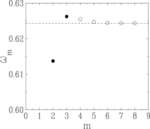
Figure 2: Plot of the probability $\omega_{m}$ that the $m$–th record node is a leader, against $m$. Full symbols: exact values (3.10) and (3.11). Empty symbols: data for higher $m$, obtained by a numerical simulation based on the recursions (2.19), (3.4) and (3.7). Dashed line: asymptotic limit given by the Golomb-Dickman constant $\omega$, eq. (4.28).

Denoting by $\nu=1,2,\dots$ the difference of the labels of any two successive leaders, say $m$ and $m+\nu$, the “reign” of the leader born at $N_{m}$, i.e., the period of time during which it stays a leader, begins at time

$$a_{m}=N_{m}+L_{m}$$ (3.12)

and ends at time

$$b_{m}=a_{m+\nu}=N_{m+\nu}+L_{m+\nu}.$$ (3.13)

The reign therefore has a duration

$$l_{m}=b_{m}-a_{m}=a_{m+\nu}-a_{m}.$$ (3.14)

The statistics of these times is addressed in section 5.

Finally, the inequalities

$$a_{m}<N_{m+1}<b_{m}$$ (3.15)

prove that the $m$–th record node is a leader (for some period of time) if and only if it leads at time $N_{m+1}$, i.e., if and only if ${\Delta}_{m+1}>L_{m}$.

3.2 Continuum theory

As stated previously, the statistics of records is faithfully described in the regime of long times by a continuum approach. The late stages of the RD growth process have a similar asymptotically exact continuum description.

In the continuum theory the key quantity is the ratio

$$R_{m}=\frac{L_{m}}{N_{m}},$$ (3.16)

which is the fraction of nodes which are connected to the leader at that time. Indeed the numerator $L_{m}$ is the degree of the leader at time $N_{m}$, while $N_{m}$ is equal to the number of nodes in the system. According to (3.6), $R_{m}$ is also the scaled maximal inter-record interval. The values taken by $R_{m}$ are clearly between 0 and 1. Recalling (2.24), the recursion (3.7) becomes

$$R_{m+1}=\max(U_{m+1}R_{m},\,1-U_{m+1}),$$ (3.17)

where $U_{m+1}$ is uniformly distributed between 0 and 1 and independent of $R_{m}$. The branches of (3.17) correspond respectively to the events

$${\cal L}_{m}=\{m\hbox{ leader}\}\hfill = \left\{U_{m+1}<\frac{1}{1+R_{m}}\right\}\Rightarrow R_{m+1}=1-U_{m+1},$$

$$\SS_{m}=\{m\hbox{ subleader}\} = \left\{U_{m+1}>\frac{1}{1+R_{m}}\right\}\Rightarrow R_{m+1}=U_{m+1}R_{m}.$$

The stochastic dynamical system defined by (3.17) plays a central role in the following. It is reminiscent of the recursions introduced by Dyson [17], then used extensively in the study of one-dimensional disordered systems [18].

4 Statistics of the leader: one-time quantities

4.1 Invariant distribution

There is an invariant distribution

$$f_{R}=\lim_{m\to\infty}f_{R_{m}}$$ (4.1)

associated with the random recursion (3.17). The latter implies a recursion between the probability densities of $R_{m}$ and $R_{m+1}$:

$$f_{R_{m+1}}=(L+S)f_{R_{m}},$$ (4.2)

where we have introduced the linear operators $L$ (leader) and $S$ (subleader), acting on a function $f(x)$ defined for $0<x<1$ as

$$Lf(x)=\int_{0}^{\min(1,x/(1-x))}\,{\rm d}uf(u),\quad Sf(x)=\int_{x}^{\min(1,x/(1-x))}\,\frac{{\rm d}u}{u}f(u).$$ (4.3)

The invariant distribution therefore obeys the fixed-point equation

$$\ f_{R}=(S+L)f_{R}.$$ (4.4)

Defining the variable $V=1/R$, with density $f_{V}(v)$ for $v>1$, eq. (4.4) can be recast as the integral equation

$$v^{2}\,f_{V}(v)=\left\{\matrix{\displaystyle\int_{1}^{v}{\rm d}u\,uf_{V}(u)+1\hfill&(1<v<2),\cr\cr\displaystyle\int_{v-1}^{v}{\rm d}u\,uf_{V}(u)+\int_{v-1}^{\infty}{\rm d}uf_{V}(u)\quad&(v>2),\hfill}\right.$$ (4.5)

which simplifies to the differential equation

$$\frac{{\rm d}}{{\rm d}v}(vf_{V}(v))=f_{V}(v)+vf_{V}^{\prime}(v)=\left\{\matrix{0\hfill&(1<v<2),\cr-f_{V}(v-1)\quad&(v>2).\hfill}\right.$$ (4.6)

We readily obtain both the explicit result

$$f_{V}(v)=\frac{1}{v}\quad(1<v<2),$$ (4.7)

and the integral relation

$$f_{V}(v)=\frac{1}{v}\int_{v-1}^{\infty}{\rm d}u\,f_{V}(u)\quad(v>2).$$ (4.8)

Transforming back to the variable $R$, we find

$$f_{R}(x)=\frac{1}{x}\int_{0}^{\min(1,x/(1-x))}\,{\rm d}uf_{R}(u).$$ (4.9)

Using (4.7) as an input, the second line of (4.6) can be solved iteratively. We thus obtain more and more complex analytic expressions for the invariant density $f_{V}(v)$ on the intervals delimited by the integers. We have $f_{V}(v)=(1-\ln(v-1))/v$ for $2<v<3$, whereas the expression for $3<v<4$ involves the dilogarithm function ${\rm Li}_{2}(2-v)$. The corresponding expressions in terms of the variable $R$ are $f_{R}(R)=1/R$ for $1/2<R<1$ and $f_{R}(R)=[1+\ln(R/(1-R))]/R$ for $1/3<R<1/2$. The invariant density $f_{V}(v)$ has weaker and weaker singularities at integer values of $v$. Using (4.6) it is readily found that the $n$–th derivative of $f_{V}(v)$ has a discontinuity at $v=n+1$ of the form

$${\Delta}f_{V}^{(n)}(n+1)=f_{V}^{(n)}(n+1^{+})-f_{V}^{(n)}(n+1^{-})=\frac{(-1)^{n}}{(n+1)!}.$$ (4.10)

Figure 3 shows a plot of the invariant density $f_{R}(R)$, obtained by a direct numerical simulation of the recursion (3.17). This procedure is more accurate than for example a numerical inversion of the explicit form (4.16) of the Laplace transform. The leading singularity at $R=1/2$ is clearly visible as the maximum of a symmetric cusp. The above expressions for the invariant density indeed yield $f^{\prime}_{R}(R=1/2\pm 0)=\mp 4$. The other singularities at $R=1/3$, $R=1/4$, etc., are not visible.

Figure 3: Plot of the invariant probability density $f_{R}(R)$. The dashed line emphasizes the symmetric cusp at $R_{\rm cusp}=1/2$.

Another consequence of the differential equation (4.6) is as follows. Multiplying both sides of these equations by $v^{p}$, where $p$ is any complex number, and integrating over $v$ gives

$$\langle V^{p}\rangle+\int_{1}^{\infty}{\rm d}v\,v^{p+1}f_{V}^{\prime}(v)=-\langle(V+1)^{p}\rangle.$$ (4.11)

An integration by parts using the initial value $f_{V}(1)=1$ coming from (4.7) leads to the identity

$$\langle(V+1)^{p}\rangle=1+p\langle V^{p}\rangle,$$ (4.12)

which holds for any complex $p$. It translates into an identity for the invariant distribution of the variable $R$ (up to a change of $p$ into its opposite)

$$\left\langle\left(\frac{R}{1+R}\right)^{p}\right\rangle=1-p\langle R^{p}\rangle.$$ (4.13)

The explicit computation of the invariant distribution is more easily performed by introducing the Laplace transform

$$\widehat{f}_{V}(s)=\langle{\rm e}^{-sV}\rangle=\int_{1}^{\infty}{\rm d}v\,f_{V}(v)\,{\rm e}^{-sv}.$$ (4.14)

Eq. (4.6) yields, using again the initial value $f_{V}(1)=1$,

$$s\,\frac{{\rm d}\widehat{f}_{V}(s)}{{\rm d}s}={\rm e}^{-s}(\widehat{f}_{V}(s)-1).$$ (4.15)

The solution of this equation reads

$$\widehat{f}_{V}(s)=1-{\rm e}^{-E(s)}=1-s\,{\rm e}^{\gamma-F(s)},$$ (4.16)

where we have introduced the functions

$$E(s) = \int_{s}^{\infty}{\rm d}u\,\frac{{\rm e}^{-u}}{u}=-{\rm Ei}(-s)=-\gamma-\ln s+F(s),$$

$$F(s) = \int_{0}^{s}{\rm d}u\,\frac{1-{\rm e}^{-u}}{u}=\sum_{k\geq 1}\frac{(-1)^{k+1}}{k\,k!}\,s^{k}$$ (4.17)

and Ei is the exponential integral function. The second expression of the function $F(s)$ shows that it is an entire function of the complex variable $s$. The moments of $V$ are readily obtained by expanding the second expression of (4.16) in powers of $s$. They are rational multiples of ${\rm e}^{\gamma}$:

$$\langle V\rangle={\rm e}^{\gamma},\quad\langle V^{2}\rangle=2\,{\rm e}^{\gamma},\quad\langle V^{3}\rangle=\frac{9}{2}\,{\rm e}^{\gamma},\quad\hbox{etc.}$$ (4.18)

Let us finally determine the behavior of $f_{V}(v)$ as $v\to\infty$, or equivalently that of $f_{R}(x)$ as $x\to 0$. This analysis is conveniently done along the lines of [19]. Anticipating a fast decay in the regime under consideration, we set

$$f_{V}(v)\sim{\rm e}^{-\phi(v)},$$ (4.19)

and approximate the integral in the right-hand side of (4.8) by

$$\int_{v-1}^{\infty}{\rm d}u\,f_{V}(u)\approx\frac{{\rm e}^{-\phi(v-1)}}{\phi^{\prime}(v-1)},$$ (4.20)

obtaining thus

$$\phi(v)-\phi(v-1)\approx\ln v+\ln\phi^{\prime}(v-1).$$ (4.21)

Setting

$${\lambda}=\ln v,\quad\phi(v)=v\,a({\lambda}),\quad b({\lambda})=a({\lambda})+\frac{{\rm d}a({\lambda})}{{\rm d}{\lambda}},$$ (4.22)

we obtain

$$b({\lambda})\approx{\lambda}+\ln b({\lambda}).$$ (4.23)

The latter equation is correct up to terms of relative order $1/v$, i.e., exponentially small in ${\lambda}$. It is therefore exact to all orders in $1/{\lambda}$. Its solution yields the asymptotic expansion

$$a={\lambda}+\mu+\frac{\mu}{{\lambda}}-\frac{(\mu-1)^{2}}{2{\lambda}^{2}}+\frac{2\mu^{3}-9\mu^{2}+12\mu-13}{6{\lambda}^{3}}+\cdots,$$ (4.24)

with the shorthand notation $\mu=\ln{\lambda}-1=\ln(\ln v)-1$. We thus obtain

$$f_{V}(v)\sim\exp\left\{-v\left(\ln v+\ln(\ln v)-1+\frac{\ln(\ln v)-1}{\ln v}+\cdots\right)\right\}.$$ (4.25)

The invariant density therefore decays faster than exponentially. It can be said to decay factorially, as the leading behavior of (4.25) is identical to that of $1/v!$.

4.2 Probability for a record node to be a leader

The knowledge of the invariant distribution $f_{R}$ allows the determination of one-time quantities in the late time regime of the process. In particular, consider the asymptotic probability $\omega$ for a record node to be a leader (for some period of time):

$$\omega=\lim_{m\to\infty}\omega_{m}=\lim_{m\to\infty}\mathop{\rm Prob}\nolimits({\cal L}_{m})=\lim_{m\to\infty}\mathop{\rm Prob}\nolimits\left(U_{m+1}<\frac{1}{1+R_{m}}\right).$$ (4.26)

Thus, using the identity (4.13) for $p=1$,

$$\omega=\left\langle\frac{1}{1+R}\right\rangle=\langle R\rangle=\int_{0}^{\infty}{\rm d}s\widehat{f}_{V}(s).$$ (4.27)

Finally, using (4.16), we obtain

$$\omega=\int_{0}^{\infty}{\rm d}s\,{\rm e}^{-s-E(s)}=\int_{0}^{1}{\rm d}x\,\exp\left(\int_{0}^{x}\frac{{\rm d}y}{\ln y}\right)=0.624\,329\,988\dots$$ (4.28)

This number is known as the Golomb-Dickman constant [20]. It first appeared in the framework of the decomposition of an integer into its prime factors [21], then in the study of the longest cycle in a random permutation of order $n$ [22, 23, 24]. The connection of the present study to the statistics of cycles of permutations will be given in section 6.1.

Eq. (4.27) shows that $\omega$ is also the mean scaled maximal inter-record interval.

4.3 Degree of the leader at a generic instant of time

The invariant distribution $f_{R}$ associated with the recursion (3.17) gives the probability distribution of the fraction of nodes which are connected to the leader at a record time, in the late-time regime. We now solve the same question when the time of observation is a generic late time.

Let an instant of time $n\gg 1$ be given. Eq. (3.5) now reads

$$L(n)=\max(L_{M},n-N_{M}),$$ (4.29)

where $M\equiv M_{n}$ is the fluctuating number of records before time $n$, and $L_{M}=\max({\Delta}_{2},\dots,{\Delta}_{M})$. Setting

$$R(n)=\frac{L(n)}{n},$$ (4.30)

equation (4.29) leads to

$$R(n)=\max(R_{M}X_{n},1-X_{n}),$$ (4.31)

where the ratio $X_{n}$, defined in (2.32), is uniformly distributed between 0 and 1 and independent of $R_{M}$ (see (2.35)). The recursion (4.31) therefore maps $R_{M}$ onto $R(n)$ in exactly the same way as the recursion (3.17) maps $R_{m}$ onto $R_{m+1}$. As a consequence, the distribution of the ratio $R(n)$ at a generic late time is also given by the invariant distribution $f_{R}$. Stated otherwise, the fraction of nodes which are connected to the leader at a record time and at a generic time are identically distributed.

4.4 Probabilities for the current record node to be a leader

Consider first the probability that the current record node at time $n$, that is, the record node number $M_{n}$, is the leader at the current time $n$. This event requires that $n-N_{M}>L_{M}$, which implies $1-X_{n}>R_{M}X_{n}$, or finally $X_{n}<1/(1+R_{M})$. The variable $R_{M}$ is asymptotically distributed according to the invariant distribution $f_{R}$, while $X_{n}$, uniformly distributed between 0 and 1, is independent of $R_{M}$. As a consequence, we find that the probability under consideration is again equal to the Golomb-Dickman constant $\omega$.

Consider now the probability that the current record node at time $n$, that is, the record node number $M_{n}$, is a leader (for some period of time). This is a different quantity, larger than the previous one. Recall that by “a given node is a leader” we mean that it leads for some duration of time. It does not necessarily lead at time $n$, but will surely lead at time $N_{M+1}$ (see (3.15)). Now the inequality to be satisfied is $N_{M+1}-N_{M}>L_{M}$, implying $Z_{n}>1+R_{M}$, where the time ratio $Z_{n}$, defined in (2.32), with probability density (2.35), is independent of $R_{M}$. The probability under consideration therefore reads

$$\Omega=\int_{0}^{1}{\rm d}R\,f_{R}(R)\int_{1+R}^{\infty}{\rm d}z\,\frac{\ln z}{z^{2}}=\left\langle\frac{1+\ln(1+R)}{1+R}\right\rangle=0.914\,063\dots$$ (4.32)

As expected, we have $\Omega>\omega$. This inequality has yet another interpretation. The probability $\Omega$ for the current record node to be a leader is larger than the probability $\omega$ for any record node to be a leader. This is so because, for a fixed time $n$, larger intervals $N_{M+1}-N_{M}$ have a higher probability to be sampled. And the later the successor of a record node is born, the higher its probability to be a leader.

5 Statistics of the leader: two-time quantities

This section is devoted to a study of two-time quantities in the process, focusing our attention onto the main characteristics of the reign of a leader, defined in section 3.1, i.e., the difference $\nu$ of the labels of two successive leaders (section 5.1), and the time ratios $N_{m+\nu}/N_{m}$, $a_{m}/N_{m}$, $b_{m}/N_{m}$, $l_{m}/N_{m}$ (section 5.2). All these quantities have limit distributions in the late-time regime.

5.1 Statistics of the difference of the labels of two successive leaders

Let us first consider the distribution of the random integer $\nu=1,2,\dots$, which is the difference of the labels of two successive leaders in the sequence of record times, $m$ and $m+{\nu}$. Hereafter we consider $m$ as being large enough, so that the process is described by the continuum formalism. We shift the record labels by $m$, so that the two leaders now have labels 0 and $\nu$. We consistently denote the invariant density $f_{R}$ by $f_{0}$. The probability for a record node to be a leader reads

$$\mathop{\rm Prob}\nolimits({\cal L}_{0})=\omega.$$ (5.1)

The distribution of ${\nu}$ is encoded in the probabilities

$$P_{n}=\mathop{\rm Prob}\nolimits(\nu=n)=\frac{1}{\omega}\,\mathop{\rm Prob}\nolimits({\cal L}_{0}\SS_{1}\dots\SS_{n-1}{\cal L}_{n}),$$

$$Q_{n}=\mathop{\rm Prob}\nolimits(\nu\geq n)=\frac{1}{\omega}\,\mathop{\rm Prob}\nolimits({\cal L}_{0}\SS_{1}\dots\SS_{n-1}).$$ (5.2)

The following relationships hold:

$$P_{n}=Q_{n}-Q_{n+1},\quad Q_{n}=\sum_{m\geq n}P_{m},$$

$$\sum_{n\geq 1}P_{n}=Q_{1}=1,\quad\langle\nu\rangle=\sum_{n\geq 1}n\,P_{n}=\sum_{n\geq 1}Q_{n}.$$ (5.3)

In order to compute the $P_{n}$ and $Q_{n}$ we consider the sequence of functions $f_{n}(x)$ defined by

$$f_{n}=S^{n-1}Lf_{0}\quad(n\geq 1),$$ (5.4)

obtained as the result of the action, upon the invariant density $f_{0}$, of the operator $L$, followed by $n-1$ successive actions of the linear operator $S$. We have

$$Q_{n}=\frac{1}{\omega}\int_{0}^{1}{\rm d}u\,f_{n}(u).$$ (5.5)

Similarly,

$$P_{n}=\frac{1}{\omega}\int_{0}^{1}{\rm d}u\,f_{n}(u)\,\frac{1}{1+u},$$ (5.6)

the factor $1/(1+u)$ being due to the last event ${\cal L}_{n}$ in the definition (5.2).

We have

$$\sum_{n\geq 1}f_{n}=(1-S)^{-1}Lf_{0}=f_{0}$$ (5.7)

since $(1-S)f_{0}=Lf_{0}$ by (4.4), or $(1-S)^{-1}Lf_{0}=f_{0}$. Eq. (5.7) has a simple interpretation: the distribution of the variable $R$ of the next leader is identical to that of the variable $R$ of the current leader. Inserting the sum rule (5.7) into (5.5) yields, using (5.3),

$$\langle\nu\rangle=\sum_{n\geq 1}Q_{n}=\frac{1}{\omega}.$$ (5.8)

This result, too, has a simple interpretation: the mean distance $\langle\nu\rangle$ between two consecutive leaders along the sequence of record times is the inverse of the probability $\omega$ for a given record to be a leader, or the inverse record breaking rate for the sequence of inter-record intervals.

We now perform the computation of the cumulative probabilities $Q_{n}$. Let

$$f_{1}=Lf_{0},$$ (5.9)

i.e., using (4.3),

$$f_{1}(x)=\left\{\matrix{1\hfill&\mbox{for }1/2\leq x\leq 1,\hfill\cr\displaystyle\int_{0}^{x/(1-x)}{\rm d}u\,f_{0}(u)\quad&\mbox{for }0\leq x\leq 1/2,\hfill}\right.$$ (5.10)

or finally, using (4.9),

$$f_{1}(x)=xf_{0}(x).$$ (5.11)

The function $f_{1}(x)$ is the initial condition for the recursion

$$f_{n+1}(x)=Sf_{n}(x)=\int_{x}^{\min(1,x/(1-x))}\,\frac{{\rm d}u}{u}f_{n}(u).$$ (5.12)

We make the change of variable $y=1/x$ and define $g_{n}(y)=f_{n}(x)$. These functions obey the recursion

$$g_{n+1}(y)=\int_{\max(1,y-1)}^{y}\,\frac{{\rm d}v}{v}g_{n}(v),$$ (5.13)

which assumes a simpler form in terms of Laplace transforms:

$$\widehat{g}_{n}(s)=-\frac{{\rm d}}{{\rm d}s}\left(\frac{s}{1-{\rm e}^{-s}}\widehat{g}_{n+1}(s)\right).$$ (5.14)

Consider the generating function of the $\widehat{g}_{n}(s)$,

$$G(x,s)=\sum_{n\geq 2}\widehat{g}_{n}(s)x^{n-1}.$$ (5.15)

From (5.14) we obtain the differential equation

$$x(G(x,s)+\widehat{g}_{1}(s))=-\frac{{\rm d}}{{\rm d}s}\left(\frac{s}{1-{\rm e}^{-s}}\,G(x,s)\right),$$ (5.16)

whose solution reads

$$G(x,s)=x\,\frac{1-{\rm e}^{-s}}{s}\,{\rm e}^{-xF(s)}\int_{s}^{\infty}{\rm d}t\,{\rm e}^{xF(t)}\,\widehat{g}_{1}(t).$$ (5.17)

Furthermore, from (5.11) it is easily found that

$$\widehat{g}_{1}(s)=-\frac{{\rm d}}{{\rm d}s}\widehat{f}_{V}(s)={\rm e}^{\gamma-s-F(s)}.$$ (5.18)

Coming back to the $Q_{n}$, we have

$$Q_{n}=\frac{1}{\omega}\int_{0}^{1}{\rm d}uf_{n}(u)=\frac{1}{\omega}\int_{1}^{\infty}{\rm d}v\,\frac{g_{n}(v)}{v^{2}}=\frac{1}{\omega}\int_{0}^{\infty}{\rm d}s\,s\,\widehat{g}_{n}(s).$$ (5.19)

Introducing the generating function of the $Q_{n}$,

$$\Sigma(x)=\sum_{n\geq 1}Q_{n}x^{n-1},$$ (5.20)

we obtain

$$\Sigma(x)=1+\frac{1}{\omega}\int_{0}^{\infty}{\rm d}s\,s\,G(x,s).$$ (5.21)

The expressions (5.17) and (5.18) yield the explicit result

$$\Sigma(x)=\frac{{\rm e}^{\gamma}}{\omega}\int_{0}^{\infty}{\rm d}s\,{\rm e}^{-xF(s)}\int_{s}^{\infty}{\rm d}t\,{\rm e}^{-t+(x-1)F(t)}.$$ (5.22)

Several results of interest can be derived from this exact expression. First of all, taking the derivative at $x=0$, we obtain

$$Q_{2}=\Sigma^{\prime}(0)=\frac{1}{\omega}\int_{0}^{\infty}\frac{{\rm d}t}{t}(t-1+{\rm e}^{-t})\,{\rm e}^{-t-E(t)}.$$ (5.23)

The integral can be evaluated to yield

$$Q_{2}=\frac{2\omega-1}{\omega},\quad\hbox{i.e.,}\quad P_{1}=\frac{1-\omega}{\omega}.$$ (5.24)

This can alternatively be obtained using (5.6) and (5.11). The probability that two successive records are leaders therefore reads $\mathop{\rm Prob}\nolimits({\cal L}_{0}{\cal L}_{1})=\omega P_{1}=1-\omega=0.375\,670\dots$ This value is close to what it would be in the absence of any correlation, namely $\omega^{2}=0.389\,788\dots$

The moments of $\nu$ can be derived by expanding (5.22) around $x=1$. We thus recover the result (5.8) for $\langle\nu\rangle$, as $\Sigma(1)=1/\omega$. For the second moment $\langle\nu^{2}\rangle$, we find

$$\langle\nu^{2}\rangle = \sum_{n\geq 1}n^{2}P_{n}=\sum_{n\geq 1}(2n-1)Q_{n}=\frac{1}{\omega}+2\Sigma^{\prime}(1)$$ (5.25)

$$= \frac{1}{\omega}\left[1+2\int_{0}^{\infty}\frac{{\rm d}s}{s}\,{\rm e}^{-E(s)}\int_{s}^{\infty}\frac{{\rm d}t}{t}\,{\rm e}^{-t}(1-{\rm e}^{-t})\right]$$

$$= 3.383\,695\dots$$

The expression (5.22) also shows that $\Sigma(x)$ has no singularity at any (finite) value of $x$. In other words, it is an entire function of the complex variable $x$. As a consequence, the $Q_{n}$ fall off at large $n$ faster than exponentially. This means that $Q_{n+1}/Q_{n}\to 0$, so that $P_{n}\approx Q_{n}$. From a quantitative viewpoint, the fall-off of the $Q_{n}$ (i.e., of the $P_{n}$) can be derived from the asymptotic behavior of $\Sigma(x)$ as $\mathop{\rm Re}\nolimits x\to+\infty$. In this regime, the double integral in (5.22) is dominated by small values of $s$, where $F(s)\approx s$, and large values of $t$, where $F(t)\approx\ln t+\gamma$. We thus obtain

$$\Sigma(x)\approx\frac{{\rm e}^{\gamma x}}{\omega x}\,\Gamma(x)\approx\frac{1}{\omega}\,\sqrt{\frac{2\pi}{x^{3}}}\,{\rm e}^{x(\ln x+\gamma-1)}\quad(\mathop{\rm Re}\nolimits x\to+\infty).$$ (5.26)

The contour integral representation of $Q_{n}$,

$$Q_{n}=\oint\frac{{\rm d}x}{2\pi{\rm i}}\,\frac{\Sigma(x)}{x^{n}},$$ (5.27)

can then be evaluated by the saddle-point method. Parametrizing the saddle-point as $x_{c}=n/a$, we are left with the estimate

$$P_{n}\approx Q_{n}\approx\frac{a}{\omega n\sqrt{a+1}}\,{\rm e}^{-n(a-\gamma-1+1/a)},$$ (5.28)

where $a$ obeys the implicit equation

$$a=\ln(n/a)+\gamma.$$ (5.29)

Setting $\lambda=\ln n+\gamma$ and $\mu=\ln\lambda=\ln(\ln n+\gamma)$, we obtain the asymptotic expansions

$$a=\lambda-\mu+\frac{\mu}{\lambda}+\frac{\mu(\mu-2)}{2\lambda^{2}}+\cdots$$ (5.30)

and

$$P_{n}\approx Q_{n}\sim\exp\left\{-n\left(\ln n-\mu-1+\frac{\mu+1}{\lambda}+\frac{\mu^{2}}{2\lambda^{2}}+\cdots\right)\right\}.$$ (5.31)

The above expansions are very similar to (4.24) and (4.25). The $P_{n}$ can again be said to decay factorially, as their leading behavior coincides with that of $1/n!$.

The accuracy of the estimate (5.28) is demonstrated in Figure 4, showing a surprisingly good agreement between this prediction and numerical data for the probability distribution $P_{n}$, obtained by a direct numerical simulation of the recursion (3.17).

Figure 4: Probability distribution of the difference of labels $\nu$ between two successive leaders. The logarithm of $P_{n}=\mathop{\rm Prob}\nolimits(\nu=n)$ is plotted against the integer $n$. Symbols: data obtained by a direct numerical simulation of the random recursion (3.17). Line: value of the asymptotic estimate (5.28), obtained by means of a numerical solution of the implicit equation (5.29).

5.2 Statistics of the lengths of time associated with the reign of a leader

We now turn to the statistics of the time ratios

$$\rho_{m}=\frac{N_{m+\nu}}{N_{m}},\quad\alpha_{m}=\frac{a_{m}}{N_{m}},\quad\beta_{m}=\frac{b_{m}}{N_{m}},\quad\lambda_{m}=\frac{l_{m}}{N_{m}},$$ (5.32)

where $N_{m}$ and $N_{m+\nu}$ are the birth times of the current leader and of the next one, and where the beginning and ending times, $a_{m}$ and $b_{m}$, and the duration of the reign $l_{m}$ of the current leader are defined in (3.12), (3.13) and (3.14).

We again shift the record labels by $m$, so that the two leaders under consideration have labels 0 and $\nu$, whereas the intermediate record nodes, labeled $m=1,\dots,\nu-1$, are not leaders. We have therefore, using (3.17)

$$R_{1}=1-U_{1},$$

$$R_{2}=(1-U_{1})U_{2},\quad\dots,$$

$$R_{\nu}=(1-U_{1})U_{2}\dots U_{\nu}.$$ (5.33)

The above time ratios can therefore be expressed in terms of the variables $R_{0}$, $R_{1}$ and $R_{\nu}$ as

$$\alpha_{0} = 1+R_{0},$$ (5.34)

$$\rho_{0} = \frac{R_{1}}{(1-R_{1})R_{\nu}},\quad\beta_{0}=\frac{R_{1}(1+R_{\nu})}{(1-R_{1})R_{\nu}}=(1+R_{\nu})\rho_{0},\quad$$ (5.35)

$$\lambda_{0} = \beta_{0}-\alpha_{0}.$$ (5.36)

These time ratios have well-defined limit distributions $f_{\alpha}$, $f_{\rho}$, $f_{\beta}$, $f_{\lambda}$ in the late-time regime. This reflects the temporal self-similarity of the process.

Figure 5 shows plots of the probability distributions $f_{\rho}$, $f_{\beta}$, $f_{\lambda}$ of the three time ratios $\rho_{0}$, $\beta_{0}$ and $\lambda_{0}$, and of the distributions $f_{1/\rho}$, $f_{1/\alpha}$, $f_{1/\lambda}$ of their inverses. The data have been obtained by a direct simulation of the recursion (3.17). The plots emphasize the following characteristics. The three distributions $f_{\rho}$, $f_{\beta}$, $f_{\lambda}$ share with the invariant distribution $f_{R}$ the property that their maxima correspond to cusps. The values at which these cusps occur, namely $\rho_{\rm cusp}=2$, $\beta_{\rm cusp}=3$ and $\lambda_{\rm cusp}=1$, are readily obtained by replacing in (5.35), (5.36) both variables $R_{1}$ and $R_{\nu}$ by $R_{\rm cusp}=1/2$. The lower plot in Figure 5 demonstrates that the distributions of the inverse time ratios have well-defined limits at zero:

$$f_{1/\rho}(0)={\cal A},\quad f_{1/\beta}(0)=f_{1/\lambda}(0)={\cal B}.$$ (5.37)

In other words, the distributions of these three time ratios fall off as $1/x^{2}$:

$$f_{\rho}(x)\approx\frac{{\cal A}}{x^{2}},\quad f_{\beta}(x)\approx f_{\lambda}(x)\approx\frac{{\cal B}}{x^{2}}.$$ (5.38)

The exact values of the amplitudes ${\cal A}$ and ${\cal B}$ will be evaluated below (see (5.49)–(5.51)). The fact that $f_{\beta}$ and $f_{\lambda}$ share the same fall-off amplitude ${\cal B}$ is simply due to the fact that the difference $\beta_{0}-\lambda_{0}=\alpha_{0}$ is bounded in the range $1\leq\alpha_{0}\leq 2$ (see (5.34)).

Figure 5: Top: plot of the probability distributions $f_{\rho}$, $f_{\beta}$, $f_{\lambda}$ of the time ratios introduced in (5.35), (5.36). Bottom: plot of the probability distributions of their inverses. Symbols: exact values ${\cal A}$ and ${\cal B}$ of the densities at the origin (see (5.49)–(5.51)). The dashed lines emphasize the cusps at $\rho_{\rm cusp}=2$, $\beta_{\rm cusp}=3$ and $\lambda_{\rm cusp}=1$.

The actual evaluation of the joint distribution of the variables $R_{1}$ and $R_{\nu}$ is now performed. The starting point is to consider the probability

$$P(r_{1},r) =\mathop{\rm Prob}\nolimits(R_{1}<r_{1},R_{\nu}<r,{\cal L}_{0}),$$ (5.39)

$$=\sum_{n\geq 1}\mathop{\rm Prob}\nolimits(R_{1}<r_{1},R_{n}<r,{\cal L}_{0}\,,{\nu}=n),$$

$$=\sum_{n\geq 1}\mathop{\rm Prob}\nolimits(R_{1}<r_{1},R_{n}<r,{\cal L}_{0}\,\SS_{1}\dots\SS_{n-1}\,{\cal L}_{n}).$$

Note that $P(1,1)=\mathop{\rm Prob}\nolimits({\cal L}_{0})=\omega$. The normalized joint density that we are looking for is thus

$$f_{R_{1},R_{\nu}}(r_{1},r)=\frac{1}{\omega}\frac{\partial}{\partial r_{1}}\frac{\partial}{\partial r}P(r_{1},r).$$ (5.40)

As in section 5.1, we start from the invariant distribution $f_{0}$. Acting on it with the operator $L$ yields $f_{1}$ (see (5.9)). We then fix the value of $R_{1}$ to $r_{1}$, thus obtaining the density $(1/\omega)f_{1}(r_{1})\delta(r-r_{1})$. We then define

$$\varphi_{1}(r_{1},r)=\delta(r-r_{1}),$$ (5.41)

and introduce the functions

$$\varphi_{n}(r_{1},r) = S^{n-1}\varphi_{1}(r_{1},r),$$

$$\varphi(r_{1},r) = \sum_{n\geq 1}\varphi_{n}(r_{1},r)=(1-S)^{-1}\varphi_{1}(r_{1},r),$$ (5.42)

where the operator $S$ acts on the variable $r$.

We are thus left with the result

$$f_{R_{1},R_{\nu}}(r_{1},r)=\frac{1}{\omega}\,f_{1}(r_{1})\varphi(r_{1},r)\,\frac{1}{1+r},$$ (5.43)

where the factor $1/(1+r)$ comes from the last event ${\cal L}_{n}$. We now make the change of variable $y=1/r$, $y_{1}=1/r_{1}$, and define $\psi_{n}(y_{1},y)=\varphi_{n}(r_{1},r)$ and $\psi(y_{1},y)=\varphi(r_{1},r)$. The Laplace transform of $\psi_{1}(y_{1},y)$ is $\widehat{\psi}_{1}(y_{1},s)=y_{1}^{2}\,{\rm e}^{-sy_{1}}$. Therefore, in analogy with (5.17), the Laplace transform of $\psi(y_{1},y)$ reads

$$\widehat{\psi}(y_{1},s)=y_{1}^{2}\left({\rm e}^{-sy_{1}}+\frac{1-{\rm e}^{-s}}{s}\,{\rm e}^{-F(s)}\int_{s}^{\infty}{\rm d}t\,{\rm e}^{F(t)-ty_{1}}\right).$$ (5.44)

The expression (5.43) of the normalized joint probability density of the variables $R_{1}$ and $R_{\nu}$ therefore contains two non-trivial factors: $f_{1}(r_{1})=g_{1}(y_{1})$, whose Laplace transform with respect to $y_{1}$ is given by (5.18), and $\varphi(r_{1},r)=\psi(y_{1},y)$, whose Laplace transform with respect to $y$ is given by (5.44). The knowledge of this distribution allows one, at least in principle, to compute the distribution of the time ratios $\rho_{0}$, $\lambda_{0}$, $\beta_{0}$ and of similar quantities. Analytical expressions thus obtained are however very cumbersome, and therefore of little use, either theoretically or practically, except for some simple examples, such as the amplitudes ${\cal A}$ and ${\cal B}$, which will now be evaluated explicitly.

Consider first the amplitude ${\cal A}$. The probability density $f_{1/\rho}$ can be expressed as

$$f_{1/\rho}(x) = \int_{0}^{1}{\rm d}r_{1}\int_{0}^{1}{\rm d}r\,f_{R_{1},R_{\nu}}(r_{1},r)\;\delta\!\left(x-\frac{(1-r_{1})r}{r_{1}}\right)$$ (5.45)

$$= \int_{0}^{1}{\rm d}r\,\frac{r}{(r+x)^{2}}\,f_{R_{1},R_{\nu}}\left(\frac{r}{r+x},r\right).$$ (5.46)

This expression simplifies in the $x\to 0$ limit to yield

$${\cal A}=f_{1/\rho}(0)=\int_{0}^{1}{\rm d}r\,f_{R_{1},R_{\nu}}(1,r)\,\frac{1}{r}=\frac{1}{\omega}\,\left\langle\frac{1}{R_{\nu}}\right\rangle_{R_{1}=1}.$$ (5.47)

We obtain similarly

$${\cal B}=f_{1/a}(0)=\int_{0}^{1}{\rm d}r\,f_{R_{1},R_{\nu}}(1,r)\,\frac{r+1}{r}=\frac{1}{\omega}\,\left\langle 1+\frac{1}{R_{\nu}}\right\rangle_{R_{1}=1},$$ (5.48)

hence the relation

$${\cal B}={\cal A}+\frac{1}{\omega}.$$ (5.49)

The explicit form of ${\cal B}$ is

$${\cal B}=\frac{1}{\omega}\int_{0}^{1}\frac{{\rm d}r}{r}\,\varphi(1,r)=\frac{1}{\omega}\int_{0}^{\infty}{\rm d}s\,\widehat{\psi}(1,s)=\frac{1}{\omega}\int_{0}^{\infty}{\rm d}t\,{\rm e}^{-t+F(t)},$$ (5.50)

where the double integral resulting from the insertion of the expression (5.44) of $\widehat{\psi}(1,s)$ has been simplified by an integration by parts. We thus obtain the numerical values

$${\cal A}=2.127\,451\dots,\quad{\cal B}=3.729\,168\dots$$ (5.51)

6 Connections to other fields

6.1 Records and cycles of permutations

As noted above, the asymptotic probability for a record node to be a leader is equal to the Golomb-Dickman constant, a number which appears in problems of combinatorical nature. It is for example the limit, when $n\to\infty$, of $\langle\Lambda_{n}\rangle/n$, where $\Lambda_{n}$ is the length of the longest cycle in a random permutation of order $n$ [22, 23, 24]. This number also appears in the framework of the decomposition of an integer into its prime factors [21].

Furthermore, as shown by Goncharov [23] and Shepp and Lloyd [24], $\Lambda_{n}/n\to\cal{R}$, where the distribution of the limiting random variable $\cal{R}$ coincides with the invariant distribution $f_{R}$ found in the present work. The identity of the asymptotic probability for a record node to be a leader and of the Golomb-Dickman constant is just the identity of $\langle R\rangle$ (see eq. (4.27)) and $\langle\cal{R}\rangle$.

We now explain the origin of the coincidences between features of the statistics of records and the cycle structure of permutations. The existence of connections between the two fields is well known [7, 25]. In particular, $M_{n}$, the number of records up to time $n$, has the same distribution as the number of cycles $C_{n}$ in a random permutation of order $n$ [7], as mentioned in section 2.1. There is actually a deeper relationship between the sequence of record times on the one hand, and the cycles of a random permutation on the other hand, which is due to the fact that the latter can be generated by the same set of indicator variables as the former.

For records, these variables are the $I_{i}$ defined in section 2.1. For cycles of permutations the construction is due to Feller [13], as we now recall. A permutation of order $n$ is constructed by a succession of $n$ decisions. Let $a_{1}$, $a_{2}$, $\ldots$, $a_{n}$ be the $n$ letters of the permutation. The position of $a_{1}$ is first chosen, with $n$ possibilities: $1\to i$. Then the position of $a_{i}$ is chosen, with $n-1$ possibilities: $i\to j$, and so on, until a cycle is formed. For example [13], with $n=8$, choosing

$$1\to 3\to 4\to 1$$

$$2\to 5\to 6\to 8\to 2$$

$$7\to 7,$$ (6.1)

generates the permutation $a_{4}\,a_{8}\,a_{1}\,a_{3}\,a_{2}\,a_{5}\,a_{7}\,a_{6}$. Define the indicator variable $J_{k}$, equal to 1 if a cycle is formed at the $k-$th step, else to 0. For this example we have $J_{3}=1$, $J_{7}=1$, $J_{8}=1$. Clearly, in general,

$$\mathop{\rm Prob}\nolimits(J_{k}=1)=\frac{1}{n-k+1},$$ (6.2)

and the $J_{k}$ are independent. Here the sequence of $J_{k}$ reads $0\,0\,1\,0\,0\,0\,1\,1$, with $\mathop{\rm Prob}\nolimits(J_{3}=1)=1/6$, $\mathop{\rm Prob}\nolimits(J_{7}=1)=1/2$, $\mathop{\rm Prob}\nolimits(J_{8}=1)=1$. Reverting the sequence of steps, we obtain $1\,1\,0\,0\,0\,1\,0\,0$ for the new indicator variable, that we denote by $I_{i}$ say, such that $\mathop{\rm Prob}\nolimits(I_{1}=1)=1$, $\mathop{\rm Prob}\nolimits(I_{2}=1)=1/2$, $\mathop{\rm Prob}\nolimits(I_{6}=1)=1/6$. One recognizes the construction of a sequence of records.

6.2 Random breaking of an interval

We have been, up to now, mainly interested in the statistics of leaders. We now address the full statistics of node degrees, within the continuum approach. Consider a fixed late record time $N_{m}$. The degrees of the earlier records read $K_{j-1}(N_{m})=N_{j}-N_{j-1}=\Delta_{j}$ for $j=2,\dots,m$. These degrees sum up to $N_{m}$, each of them representing a finite fluctuating fraction of the total, or “weight” $\Delta_{j}/{N_{m}}$. We have

$$\frac{\Delta_{m}}{N_{m}}=1-U_{m},$$

$$\frac{\Delta_{m-1}}{N_{m}}=U_{m}(1-U_{m-1}),$$

$$\frac{\Delta_{m-2}}{N_{m}}=U_{m}U_{m-1}(1-U_{m-2}),\quad\dots$$ (6.3)

Relabeling the indices $j\to k=m-j+1$, and denoting the weights by $W_{k}$, we have

$$W_{1}=1-U_{1},$$

$$W_{2}=U_{1}(1-U_{2}),$$

$$W_{3}=U_{1}U_{2}(1-U_{3}),\quad\dots$$ (6.4)

We recognize the sequence of weights obtained by randomly breaking an interval of unit length into two pieces, and iterating the process [26].

A convenient tool to investigate this kind of fluctuating weights consists in introducing the reduced moments

$$Y^{(p)}_{m}=\sum_{j=2}^{m}\left(\frac{\Delta_{j}}{N_{m}}\right)^{p}=\sum_{k=1}^{m-1}W_{k}^{p},$$ (6.5)

where the order $p=1,2,\dots$ is any integer [26]. These moments obey the random recursion

$$Y^{(p)}_{m+1}=U_{m+1}^{p}Y^{(p)}_{m}+(1-U_{m+1})^{p}.$$ (6.6)

The latter can be viewed as a generalization of the recursion (3.17) to any finite integer order $p$. Eq. (3.17) is formally recovered in the $p\to\infty$ limit, where the sum in (6.5) is dominated by its largest term, that is by the contribution of the leader. The $Y^{(p)}_{m}$, which keep fluctuating in the late-time regime, have non-trivial limit distributions, invariant under the dynamical system (6.6). A plot of $Y^{(2)}_{m}$, obtained by iterating (6.6) numerically, as well a plot of the invariant measure $f_{R}$ of the largest weight can be found in [26]. In the framework of the random breaking of an interval, $\omega$ is either the probability that the first weight $W_{1}$ be the largest, or the mean maximal weight.

6.3 Relation to the Kesten variable

It turns out that the invariant distribution of the random variable $R$ can be worked out more generally for a one-parameter family of problems containing the above as a special case. Consider the recursion (3.17) where the i.i.d. random variables $U_{m+1}$ have an arbitrary distribution between 0 and 1, with density $\rho(u)$. The invariant distribution still obeys the fixed-point equation (4.4), with the definitions

$$Sf(x) = \int_{x}^{\min(1,x/(1-x))}\,\frac{{\rm d}u}{u}\,\rho\!\left(\frac{x}{u}\right)\,f(u),$$

$$Lf(x) = \rho(1-x)\int_{0}^{\min(1,x/(1-x))}\,{\rm d}uf(u).$$ (6.7)

The integral equation thus obtained cannot be solved in closed form in general. It nevertheless leads to a differential equation similar to (4.6), and is therefore solvable, whenever the density of the variables $U_{m+1}$ is a power law. More precisely, if

$$\rho(u)=bu^{b-1},$$ (6.8)

where $b$ is an arbitrary positive parameter, one has

$$\frac{{\rm d}}{{\rm d}v}\left(\frac{v^{b}}{(v-1)^{b-1}}f_{V}(v)\right) = \frac{v^{b-1}}{(v-1)^{b}}\left[(v-b)f_{V}(v)+v(v-1)f_{V}^{\prime}(v)\right]$$ (6.9)

$$= \left\{\matrix{0\hfill&(1<v<2),\cr-bf_{V}(v-1)\quad&(v>2).\hfill}\right.$$

Consider the modified Laplace transform

$$\widetilde{f}_{V}(s)=\langle V^{b}\,{\rm e}^{-sV}\rangle=\int_{1}^{\infty}{\rm d}v\,v^{b}\,{\rm e}^{-sv}\,f_{V}(v).$$ (6.10)

This quantity obeys the differential equation

$$s\,\frac{{\rm d}\widetilde{f}_{V}(s)}{{\rm d}s}=-(s+b(1-{\rm e}^{-s}))\widetilde{f}_{V}(s),$$ (6.11)

whose normalized solution reads

$$\widetilde{f}_{V}(s)=\frac{\Gamma(b+1)}{s^{b}}\,{\rm e}^{-s-bE(s)}=\Gamma(b+1)\,{\rm e}^{b\gamma}\,{\rm e}^{-s-bF(s)}.$$ (6.12)

The probability $\omega$ (see eq. (4.26)) generalizes to

$$\omega(b)=\lim_{m\to\infty}\mathop{\rm Prob}\nolimits(1-U_{m+1}>U_{m+1}R_{m})=\left\langle\left(\frac{1}{1+R}\right)^{b}\right\rangle,$$ (6.13)

that is

$$\omega(b)=\left\langle\left(\frac{V}{V+1}\right)^{b}\right\rangle=\frac{1}{\Gamma(b)}\int_{0}^{\infty}{\rm d}s\,s^{b-1}\,{\rm e}^{-s}\,\widetilde{f}_{V}(s),$$ (6.14)

i.e., finally

$$\omega(b)=\int_{0}^{\infty}{\rm d}s\,{\rm e}^{-s-bE(s)}.$$ (6.15)

The original problem with a uniform distribution of the variables $U_{m+1}$ is recovered by setting $b=1$ in the above results. One has indeed $\widetilde{f}_{V}(s)=-{\rm d}\widehat{f}_{V}(s)/{\rm d}s$, and an integration by parts shows that (6.12) is equivalent to (4.16). Finally, the expression (6.15) for $\omega(1)$ coincides with the expression (4.28) of the Golomb-Dickman constant.

It can be checked that $\omega(b)=\langle R\rangle$ for all values of $b$. This identity generalizes (4.27). However, $\lim_{m\to\infty}\mathop{\rm Prob}\nolimits(1-U_{m+1}>U_{m+1}R_{m})$ and $\langle R\rangle$ are not equal for an arbitrary distribution $\rho(u)$.

The above family of exactly solvable invariant densities is in correspondence with the following problem. Consider the Kesten variable [27, 28], defined as

$$Z=1+x_{1}+x_{1}x_{2}+x_{1}x_{2}x_{3}+\cdots,$$ (6.16)

where the $x_{m}$ are i.i.d. positive random variables with probability density $\rho^{({\rm Kes})}(x)$. If this distribution is such that $\langle\ln x\rangle<0$, the sum in (6.16) is convergent and $Z$ has a well-defined probability density $f_{Z}^{({\rm Kes})}(z)$, solution of the integral equation

$$f_{Z}^{({\rm Kes})}(z)=\int_{0}^{\infty}\frac{{\rm d}x}{x}\,\rho^{({\rm Kes})}(x)\,f_{Z}^{({\rm Kes})}\!\left(\frac{z-1}{x}\right),$$ (6.17)

This equation again cannot be solved in closed form in general. It is however known [28, 29] that the problem can be solved whenever the density of the variables $x_{m}$ is a power law on an interval $[0,a]$. In the marginal situation ($a=1$) where the $x_{m}$ are between 0 and 1, with density

$$\rho^{({\rm Kes})}(x)=bx^{b-1},$$ (6.18)

where $b$ is again an arbitrary positive parameter, the Laplace transform $\widehat{f}_{Z}^{({\rm Kes})}(s)=\langle{\rm e}^{-sZ}\rangle$ has the closed-form expression

$$\widehat{f}_{Z}^{({\rm Kes})}(s)={\rm e}^{-s-bF(s)}.$$ (6.19)

The similarity between the two problems is now patent by comparing (6.12) and (6.19). The probability densities of the variable $V=1/R$ and of the Kesten variable $Z$ are related to each other by the equation

$$x^{b}\,f_{V}(x)=\Gamma(b+1)\,{\rm e}^{b\gamma}\,f_{Z}^{({\rm Kes})}(x).$$ (6.20)

7 Conclusion

The main goal of this work has been to put forward the Record-driven growth process. This ballistic growth model entirely based on the record process has been met as the zero-temperature limit of a class of network growth models with preferential attachment. Its simplicity and its minimality however suggest that the RD growth process might be relevant to a wider class of situations, besides the realm of complex networks. The main emphasis has been put on the interplay between records (i.e., nodes endowed with the best intrinsic qualities) and leaders (i.e., nodes whose degrees are the largest). The RD growth process provides a natural playground where subtle questions related to the statistics of leaders and of lead changes can be addressed in a quantitative way.

The RD growth process inherits from the record process some relationships with combinatorical problems related to permutations. Relationships with fragmentation models and with one-dimensional disordered systems have also been underlined. A key feature of the RD growth process is its temporal self-similarity in the late-time regime, inherited from the underlying record process, which manifests itself in that various time ratios have non-trivial limiting distributions in the regime of late times. This regime is also characterized by the very fast fall-off of temporal correlations.

Let us point out the recent work [30], which addresses the statistics of records for the successive positions of a random walk. The mean longest duration of a record scales with the number of steps, the ratio defining a non-trivial constant $0.626\,508\dots$ This parallels the scaling of the mean maximal inter-record interval of the present work, resulting in the occurrence of the Golomb-Dickman constant $0.624\,329\dots$

To close up, it is worth looking back to our starting point, namely the growing networks with preferential attachment considered in the Introduction. The self-similar growth regime of the RD process can be shown to be unstable against thermal fluctuations. This regime crosses over to a complete freeze-out at a time scale which usually diverges at a power-law at low temperature, as $\tau\sim T^{-b}$. The model-dependent exponent $b$ can be evaluated by generalizing the line of thought of the recent work [31], whether or not the model has a finite-temperature condensation transition.

Acknowledgments

It is a pleasure for us to thank Ginestra Bianconi for stimulating discussions.

References

References

- [1] Barabási A L and Albert R, 1999 Science 286 509
- [2] Albert R and Barabási A L, 2002 Rev. Mod. Phys. 74 47
- [3] Dorogovtsev S N and Mendes J F F, 2003 Evolution of Networks (Oxford: Oxford University Press)
- [4] Boccaletti S, Latora V, Moreno Y, Chavez M and Hwang D U, 2006 Phys. Rep. 424 175
- [5] Barrat A, Barthélemy M and Vespignani A, 2008 Dynamical Processes on Complex Networks (Cambridge: Cambridge University Press)
- [6] Bianconi G and Barabási A L, 2001 Europhys. Lett. 54, 439 Bianconi G and Barabási A L, 2001 Phys. Rev. Lett. 86 5632
- [7] Renyi A, 1962 Proceedings Coll. Combinatorial Methods in Probability Theory (Math. Inst. Aarhus Univ., Aarhus, Denmark)
- [8] Glick N, 1978 Amer. Math. Month. 85 2
- [9] Arnold B C, Balakrishnan N and Nagaraja H N, 1998 Records (New York: Wiley)
- [10] Nevzorov V B, 2001 Records: Mathematical Theory Translation of Mathematical Monographs 194 (Providence, RI: American Mathematical Society)
- [11] Krapivsky P L and Redner S, 2002 Phys. Rev. Lett. 89 258703
- [12] Graham R L, Knuth D E and Patashnik O, 1994 Concrete Mathematics (Reading, MA: Addison-Wesley)
- [13] Feller W, 1968 An Introduction to Probability Theory and its Applications (New York: Wiley)
- [14] Cox D R, 1962 Renewal theory (London: Methuen)
- [15] Cox D R and Miller H D, 1965 The Theory of Stochastic Processes (London: Chapman & Hall)
- [16] Godrèche C and Luck J M, 2001 J. Stat. Phys. 104 489
- [17] Dyson F J, 1953 Phys. Rev. 92 1331
- [18] Luck J M, 1992 Systèmes désordonnés unidimensionnels (in French) (Collection Aléa-Saclay)
- [19] Luck J M and Nieuwenhuizen T M, 1988 J. Stat. Phys. 52 1
- [20] Finch S R, 2003 Mathematical Constants (Cambridge: Cambridge University Press) Weisstein W E, Golomb-Dickman constant Mathworld http://mathworld.wolfram.com
- [21] Dickman K, 1930 Arkiv för Mat., Astron. och Fys. 22 1
- [22] Golomb S W, 1963 Bull. Amer. Math. Soc. 70 747
- [23] Goncharov W, 1944 Izv. Akad. Nauk SSSR 8 3 English translation: 1962 Amer. Math. Soc. Transl. 19 1
- [24] Shepp L A and Lloyd S P, 1966 Trans. Amer. Math. Soc. 121 340
- [25] Goldie C M, 1989 Math. Proc. Camb. Phil. Soc. 106 169
- [26] Derrida B and Flyvbjerg H, 1987 J.Phys. A 20 5273
- [27] Kesten H, 1973 Acta Math. 131 208
- [28] de Calan C, Luck J M, Nieuwenhuizen T M and Petritis D, 1985 J. Phys. A 18 501
- [29] Vervaat W, 1979 Adv. Appl. Prob. 11 750
- [30] Majumdar S N and Ziff R M, 2008 Phys. Rev. Lett. 101 050601
- [31] Ferretti L and Bianconi G, 2008 arXiv:0804.1768 to appear in Phys. Rev. E