Finding rare objects and building pure samples: Probabilistic quasar classification from low resolution Gaia spectra

Abstract

We develop and demonstrate a probabilistic method for classifying rare objects in surveys with the particular goal of building very pure samples. It works by modifying the output probabilities from a classifier so as to accommodate our expectation (priors) concerning the relative frequencies of different classes of objects. We demonstrate our method using the Discrete Source Classifier, a supervised classifier currently based on Support Vector Machines, which we are developing in preparation for the Gaia data analysis. DSC classifies objects using their very low resolution optical spectra. We look in detail at the problem of quasar classification, because identification of a pure quasar sample is necessary to define the Gaia astrometric reference frame. By varying a posterior probability threshold in DSC we can trade off sample completeness and contamination. We show, using our simulated data, that it is possible to achieve a pure sample of quasars (upper limit on contamination of 1 in 40 000) with a completeness of 65% at magnitudes of G=18.5, and 50% at G=20.0, even when quasars have a frequency of only 1 in every 2000 objects. The star sample completeness is simultaneously 99% with a contamination of 0.7%. Including parallax and proper motion in the classifier barely changes the results. We further show that not accounting for class priors in the target population leads to serious misclassifications and poor predictions for sample completeness and contamination. We discuss how a classification model prior may, or may not, be influenced by the class distribution in the training data. Our method controls this prior and so allows a single model to be applied to any target population without having to tune the training data and retrain the model.

1 Introduction

Finding rare objects is hard, for two reasons. First, we expect to have to look at many objects before we encounter one, and second, we may not even recognise it even when we do. The reason for this is that the prior probability that any one object is of the rare class, $P(C_{\rm rare})$, is very small. So even if it has very characteristic features, i.e. the likelihood of the data given the rare object, $P({\rm Data}\,|\,C_{\rm rare})$, is high, the posterior probability, $P(C_{\rm rare}\,|\,{\rm Data}$), could still be low.

A survey for rare objects obviously requires a very discriminating classifier, but we could assist it by modifying the class probabilities. If we raised the prior, $P(C_{\rm rare})$, we are more likely to find the rare objects, but it is inevitable that we will then incorrectly classify other objects as being of the rare class. Depending on our goals, there may be a satisfactory balance between maximizing the expected number of true positives (sample completeness) and minimizing the expected number of false positives (sample contamination). Here we present a method for achieving an optimal balance and a correct prediction of this balance which, although simple, is not trivial and has important implications.

We illustrate our method in the context of the problem of detecting quasars in the Gaia survey based on their low resolution ($R\simeq 30$) optical spectra. Gaia is an all-sky astrometric and spectrophotometric survey complete to $G=20$, expecting to observe some $10^{9}$ stars, a few million galaxies and half a million quasars. Its primary mission is to study Galactic structure by measuring the 3D spatial distribution and 2D kinematic distribution of stars throughout the Galaxy and correlating these with stellar properties (abundances, ages etc.) derived from the spectra. With astrometric accuracies as good as 10 $\mu$as, Gaia cannot be externally calibrated with an existing catalogue. Instead it must observe a large number of quasars over the whole sky with which to define its own reference frame. This quasar sample must be very clean (low contamination). (The quasar sample is also, of course, of intrinsic interest.)

We present our Gaia classification model, the Discrete Source Classifier (DSC), and report its classification performance using simulated data. We will show how, using our probabilty modification approach, we can use this to build pure quasar samples, at the (acceptable) loss of sample completeness.

Related work. One of the most comprehensive search for quasars to date is that done with the SDSS. Richards et al. richards02 (2002) defined a colour locus in the ugriz space to identify objects for spectroscopic follow up and estimated the contamination rate of their photometric selection to be 34%. Using the spectroscopy of all point sources taken in SDSS stripe 82, Vanden Berk et al. vandenberk05 (2005) assessed the completeness of the Richards et al. selection at 95.7% for sources brighter than $i=19.1$. Later, Richards et al. richards04 (2004) trained a photometric classifier (based on kernel density estimation) on a set of 22,000 spectroscopically identified quasars and used this to build a sample of 100 000 quasars brighter than $g=21.0$. For the unresolved UV excess quasars in this sample, they estimated the completeness to be 94.7% down to $g$=19.5, with a contamination of just 5% down to $g$=21.0. Suchkov et al. suchkov05 (2005) and Ball et al. ball06 (2006) both use decision trees to classify objects in the SDSS photometric catalogue, by training on objects with spectroscopic classifications from SDSS. Gao et al. gao08 (2008) used support vector machines and Kd-tree nearest neighbours to classify spectroscopically-confirmed SDSS and 2MASS objects as quasars or stars using just the photometry, with stars and quasars present in equal proportions. With both methods they obtained contamination rates of a few percent (averaged across both classes).

Outline. We start in section 2 by presenting our general prior modification method. In section 3 we present the Gaia-DSC classifier and the data used to train and test it. The performance of this and the application of our method are given in section 4 and discussed in section 5, where we also discuss the interpretation of the probabilities and some of the limitations of this work. We conclude in section 6.

Definitions and notation. We use the term class fractions to mean the relative numbers of objects of each class in a data set. The nominal model refers to the classifier “as is”, i.e. the output probabilities without any modifications. In contrast, in the modified model we have modified these outputs to be appropriate to a situation in which there would be very different class fractions, e.g. quasars very rare (section 2.4). The subscript $i$ refers to true classes and the subscript $j$ to model output classes. $f^{train}_{i}$, $f^{test}_{i}$ and $f^{mod}_{i}$ refer to the class fractions of class $i$ for the training data, test data and effective test data respectively. They are normalized, $\sum_{i}f^{train}_{i}=\sum_{i}f^{test}_{i}=\sum_{i}f^{mod}_{i}=1$. This effective test data set is one which we don’t actually have, but reflects a target population with different class fractions, e.g. quasars very rare. We make predictions of the performance on this by using the actual test data but by modifying the performance equations (section 2.5). In the figures especially, lower case class names, e.g. quasar, denote estimated classes and upper case names, e.g. STAR, true classes. Thus $P({\tt quasar}|{\tt STAR})$ means “the DSC-assigned quasar probability given that the source is truly a STAR”. This refers to DSC outputs for objects with known classes (e.g. in a test set). This is not to be confused with the notation for the DSC outputs in the general case, $P(C_{j}|x_{n},\theta)$, which means “the probability which DSC model $\theta$ assigns to class $C_{j}$ for object $x_{n}$”. “C&C” stands for “completeness and contamination”.

2 Using and modifying probabilities for classification

2.1 The issue of priors

The probabilities and assigned classes from any classifier depend not only on the evidence in the data, but also on the prior probabilities. In this context, the prior is the class probabilities before you look at the data. Priors are always present (whether you accept the Bayesian philosophy or not), but they are not explicit in many models, so we may not know what they are. This is a problem, because if the model priors are inappropriate (e.g. equal probability of star and quasar) this will translate into poor posterior probabilities and thus class assignments. The method we present here allows us to replace priors (even if implicit) with something more appropriate, e.g. quasars much rarer than stars.

2.2 Building samples and assessing completeness and contamination

DSC assigns to every data vector (e.g. spectrum), $x_{n}$, a probability, $P({\tt quasar})$, that it is a quasar, and likewise for the other classes. The classes are exclusive and exhaustive, so the probabilities sum to unity. The classifier is not perfect, so generally $P({\tt quasar}|{\tt QUASAR})<1$ and $P({\tt quasar}|not\,{\tt QUASAR})>0$.

We could simply assign an object to that class for which the DSC output is largest (the most probable class). However, if the different output probabilities for an object were all similar this would not be a confident classification. A more secure basis for building pure samples is to select objects only if their probability is above some threshold: the higher this is, the lower the sample contamination, but the smaller also its completeness.

We assess the performance using a labelled test set. To build a sample for class ${\tt class}$, we select objects which have a DSC output $P({\tt class})>P_{\rm t}$, where $P_{\rm t}$ is a user-defined threshold (and may be different for each class). The sample completeness is the number of objects in the sample which are truly of that class divided by the total number of objects of that class in the test set. The contamination is the number of objects in the sample which are truly of other classes divided by the total number of objects in the sample. For ${\tt class}=j$

$${\mathrm{c}ompleteness}_{j} = \frac{n_{i=j,j}}{N_{i}}$$

$${\mathrm{c}ontamination}_{j} = \frac{\sum_{i\neq j}n_{i,j}}{\sum_{i}n_{i,j}}$$ (1)

where $n_{i,j}$ is the number of objects of (true) class $i$ in the sample selected for (output) class $j$, and $N_{i}$ is the total number of objects of (true) class $i$ in the test set. (There are various other diagnostics one could use, such as the ROC curve or precision rate.) These equations give us predictions of the completeness and contamination for a new (unlabelled) data set, insofar as we believe it to have the same class fractions as the training data (that’s our prior).

2.3 Model-based class priors

All classifiers include a prior, whether explicit or not. We need to know this prior for two reasons. First, we would like to know what assumption our model is actually making (and not what we suspect it is making). Second, we would like to change this prior to something which is appropriate to the problem at hand. Here we discuss what the prior is, how the training data may influence it, and how to calculate it post hoc from a trained model.

2.3.1 Bayes and priors

The outputs from a trained classifier when presented with data $x_{n}$ are $P(C_{j}|x_{n},\theta)$, the probability that the data is of class $C_{j}$ given the data and the model, $\theta$. This latter quantity reflects both the architecture of the model and the training data set used to fix its internal parameters. We can think of this output as a posterior probability and write it using Bayes’ theorem

$$P(C_{j}|x_{n},\theta)=\frac{P(x_{n}|C_{j},\theta)P(C_{j}|\theta)}{P(x_{n}|\theta)}$$ (2)

The term $P(x_{n}|C_{j},\theta)$ is the likelihood of the data given the class and model. The term $P(C_{j}|\theta)$ is the prior probability that, given our model, an object is of class $C_{j}$. Bayesian statistics deals with updating probabilities based on new data: the prior reflects our knowledge (based on some other data) before we look at the new data. In the present context, the prior $P(C_{k}={\tt quasar}|\theta)$ is the probability that any one object in our survey is a quasar, before we look at its spectrum. We always have some prior information, e.g. with Gaia the fact that it is an all sky survey to G=20.0. If we know them, we could even treat the magnitude and Galactic latitude as prior information.

2.3.2 What are the classifier priors and how does the training data influence them?

Given that we can make the decomposition in equation 2, it follows that all classification models must possess a prior on the class probabilities. In some models, for example linear discriminant analysis or Gaussian mixture models, this prior is explict and so can be controlled. But in many others, such as neural networks or support vector machines, it is not explicit. (See a standard text on machine learning for details of these methods, e.g. Hastie et al. hastie01 (2001).) In particular, it may depend on the class fractions in the training data.

Take, for example, a standard neural network regression model which is trained by minimizing an error function over the whole data set. If we trained this on 1000 stars and just one quasar, it will learn to recognise stars much better than quasars, because in minimizing the error it hardly has to worry about fitting the lone quasar. If we changed the training data (class fractions), the model and thus the classifications would change. Other regression models are influenced by the class fractions in different ways, or not at all. Given this dependence on the model and data, we refer to the priors as model-based priors, and the notation $P(C_{j}|\theta)$ reminds us of this.

This issue of class fractions influencing the model performance is well-known in the machine learning literature, where it is referred to as the problem of “class imbalance” or “imbalanced data sets”. It has been demonstrated to influence neural networks, support vector machines and classification trees (e.g. Shin & Cho 2003, Visa & Ralescu 2005, Weiss 2004). But how, exactly, do the class fractions affect the classifications and, more specifically, the model-based priors? We might think that in the above example the ratio of the star to quasar prior probabilities implicit in the model is 1000 to 1, but this is generally not the case, because it depends on the model and how it is trained. The bottom line is that, in general, the model-based prior is not equal to the class fractions in the training data.

2.3.3 Calculating the model-based priors

We can calculate the model-based priors, $P(C_{j}|\theta)$, directly from the trained model via the marginalization equation

$$P(C_{j}|\theta)=\sum_{n=1}^{n=N_{test}}P(C_{j}|x_{n},\theta)P(x_{n}|\theta)$$ (3)

where the sum is taken over all $N_{test}$ objects in the test data set. The first term in the sum is the posterior probability. The second term is the probability that we draw object $x_{n}$ from the test data set, which is $1/N_{test}$. Hence the prior is simply the average of the posterior probabilities. It might seem strange that the prior can be calculated from the posterior. Yet because the sum is over all objects in the test set, regardless of their true class, we can think of this summation as eliminating information on individual objects, leaving us with what the model probability is for class $C_{j}$ in the absence of specific data. This is the prior. If we had three classes equally represented in the data, and the classifier were perfect, the prior for each class would be $1/3$. Different class fractions and non-perfect classifiers will give different results.

In section 4 we will compare the model-based priors with the training data class fractions.

2.4 Modifying the posterior probabilities to account for modified class fractions or priors

Typically we train a classification algorithm on more or less equal class fractions, because this helps the algorithm to reliably identify the class boundaries. This is our nominal model, $\theta^{nom}$. Yet the target population to which we want to apply our classifier may have different class fractions (e.g. quasars very rare), in which case the classifier may make poor predictions. The underlying issue here is that the model-based priors of our nominal model differ from our target priors.

To correct for this we would ideally just replace the original (nominal) prior with our modified prior. But we cannot do this directly because the model priors are not explicit. Instead we modify the output (posterior) probabilities to give us the “modified model”, $\theta^{mod}$. From inspection of equation 2 we see we may achieve this by dividing the posterior by the nominal prior and then multiplying it by the modified prior. The nominal priors can be calculated using equation 3. But we cannot use this equation to calculate the modified priors because we don’t yet have the posteriors from the modified model. We therefore approximate the modified priors using the class fractions. Let $P^{nom}(C_{j}|x,\theta^{nom})$ be the output (posterior) probability from the nominal model, i.e. that trained on the data set with class fractions ${f^{train}_{i}}$. The modified probability appropriate for a target population with class fractions $f^{mod}_{i}$ we define as

$$P^{mod}(C_{j}|x_{n},\theta^{mod})=a_{n}\,P^{nom}(C_{j}|x_{n},\theta^{nom})\,\frac{f^{mod}_{i=j}}{f^{train}_{i=j}}$$ (4)

where $a_{n}$ is a normalization factor which ensures that $\sum_{j}P^{mod}(C_{j}|x_{n},\theta^{mod})=1$ for each object $n$. The factor ${f^{mod}_{i=j}}/{f^{train}_{i=j}}$ is equivalent to changing the prior in equation 2 and has the expected impact on the posterior.

Following the discussion in section 2.3 we do not necessarily expect the class fractions to be a good proxy for the priors, but for now it’s the best we can do. (We will later check how good the approximation is.)

We illustrate the above with a simple example, a two-class model trained on equal numbers of stars and quasars, i.e. $f^{train}=(0.5,0.5)$. Let’s suppose an object is classified with the nominal model to give $P^{nom}(C_{star}|x_{n},\theta^{nom})=0.2$ and therefore $P^{nom}(C_{quasar}|x_{n},\theta^{nom})=0.8$. If we want $f^{mod}=(0.9,0.1)$ (stars nine times more common than quasars), then from equation 4 we get

$$P^{mod}(C_{star}|x_{n},\theta^{mod})=a_{n}\,0.2\times 0.9/0.5=a_{n}\,0.36=0.69$$

$$P^{mod}(C_{quasar}|x_{n},\theta^{mod})=a_{n}\,0.8\times 0.1/0.5=a_{n}\,0.16=0.31$$

the final values being those after normalization. We see how the prior can have a significant effect on our inference.

It is tempting to think of these modified probabilites as those we would have obtained if we had trained the model on the modified class fractions. But this is generally not true, because what we are doing in equation 4 is changing the priors (via the proxy of the class fractions) and this is not equivalent to changing the training data (as we will demonstrate later).

2.5 Predicting performance and model-based priors for an effective test set using the nominal test set

2.5.1 The completeness and contamination calculation

The equations for the completeness and contamination (eqn. 1) depend on the actual number of objects correctly and incorrectly classified and were calculated from the test data set, which by definition has class fractions $f^{test}_{i}$. However, we expect to apply the modified model to a target population with different class fractions (this was the whole point of modifying it). To estimate the C&C, it is not necessary to create a new test data set. Instead, we can modify the equations to reflect the target class fractions, $f^{mod}$, namely

$${\mathrm{c}ompleteness}_{j} = \frac{\left(\frac{f^{mod}_{i=j}}{f^{test}_{i=j}}\right)n_{i=j,j}}{\left(\frac{f^{mod}_{i=j}}{f^{test}_{i=j}}\right)N_{i}}=\frac{n_{i=j,j}}{N_{i}}$$

$${\mathrm{c}ontamination}_{j} = \frac{\sum_{i\neq j}\left(\frac{f^{mod}_{i}}{f^{test}_{i}}\right)n_{i,j}}{\sum_{i}\left(\frac{f^{mod}_{i}}{f^{test}_{i}}\right)n_{i,j}}$$ (5)

This effectively changes the number of objects in each true class. The quantities $n_{i,j}$ and $N_{i}$ refer to the number of objects in samples obtained from the modified model applied to the actual test data set. Note that the equation for the completeness remains unchanged, yet the value of the completeness will generally change because the posterior probabilities have changed and so $n_{i=j,j}$ changes. We emphasise that the above equation is independent of the procedure to modify the probabilities described in section 2.4. It is only to be used to make predictions for an effective test set. To calculate the completeness and contamination for an actual test set which already has the modified class fractions, we use equation 1.

2.5.2 The model-based prior calculation

Once we have the posteriors from the modified model we can calculate its model-based priors from the test set using equation 3. But just as for the C&C calculation, we must change the effective number of objects in each true class to represent the modified class fractions. Thus in equation 3 we should use

$$P(x_{n}|\theta^{mod})=\left(\frac{f^{mod}_{i}}{f^{test}_{i}}\right)\frac{1}{N_{test}}$$ (6)

where $x_{n}$, being an object in the (labelled) test set, has known true class, $i$. If a class is ten times rarer in the modified population, then $P(x_{n}|\theta^{mod})$ is reduced by a factor of ten compared to before.

In principle we could now use these model-based priors to recalculate the posteriors for the modified model (without using the approximation in equation 4), but we don’t do this in the present article. Rather we just report them as a check on what the prior really is.

3 The Discrete Source Classifier

The Discrete Source Classifier (DSC) is the algorithm we are developing as part of our work in the Gaia Data Processing and Analysis Consortium (DPAC) (O’Mullane et al. omullane07 (2007)). DSC will classify objects based primarily on low resolution prism spectra (so-called “BP/RP” spectra), but supplemented with parallaxes and proper motions and photometric variability where available. Here we restrict ourselves to the three classes “star”, “galaxy” and “quasar”. After DSC in the pipeline come several algorithms for estimating astrophysical parameters, e.g. stellar parameters. For more details of the classification system, see Bailer-Jones cbj05 (2005).

Gaia detects objects in a very broad band, G, which has roughly the same wavelength range as the BP/RP instrument. In common with the Gaia detection strategy, DSC only operates on point sources (i.e. makes no use of morphological information). In this paper we present results for simulations at both G=20.0 and G=18.5.

Here we describe the underlying classifier, the source libraries and the Gaia simulated data used to train and test DSC.

3.1 The SVM classification algorithm

DSC is presently based on a Support Vector Machine (SVM) (e.g. Cortes & Vapnik cortes95 (1995), Burges burges98 (1998)), using the libSVM implmentation (Chang & Lin libsvm (2001)). An SVM is a supervised learning algorithm which finds the boundary which “optimally” separates two classes of objects. In contrast to many other classifiers, SVMs are defined only by those training objects which lie close to the boundary, the so-called support vectors. The basic algorithm is linear, but by using the “kernel trick” to implicitly map data into a higher dimensional space, it achieves a nonlinear mapping between the input data (the spectrum) and the output classes. The SVM is trained by minimizing the number of misclassifications and using a regularizer for complexity control.

SVMs are fundamentally non-probabilistic: they simply define a boundary and assign a class ($C_{1}$ or $C_{2}$) depending on which side of the boundary an object falls. Probabilities may be derived from the distance, $f$, of an object from the boundary, in the present case by fitting a sigmoidal function to $P(C_{j}=C_{1}|f)$ (Platt platt99 (2000)).

The basic SVM is a two-class classifier. libSVM actually trains $K(K-1)/2$ one-against-one classifiers (for a $K$ class problem) and uses the pairwise coupling method described in Wu et al. wu04 (2004) (their algorithm 2) to produce normalized probabilities for $K$ classes.

One of the advantages of SVMs over many other nonlinear classifiers (e.g. neural networks) is that the SVM objective function is convex, so the training has a unique solution. However, the model has two hyperparameters, the regularization parameter (the “cost”) and the scale length in the radial basis function (RBF) kernel we use. We optimize these (“tune”) using a Nelder-Mead algorithm. As this involves retraining the SVM for each combination of hyperparameters, it is a time-consuming process.

The main concepts presented in this paper are not dependent on the choice of classifier. SVM is not perfect, not least because its underlying philosophy of not modelling the data distribution means that probabilties do not arise naturally. It is, nonetheless, a competitive model in terms of classification error, and in tests we have done it has performed as well as or better than several alternatives, including multilayer perceptrons, RBF networks, boosted trees and mixture models (Elting & Bailer-Jones elting07 (2007)).

3.2 Source spectral libraries

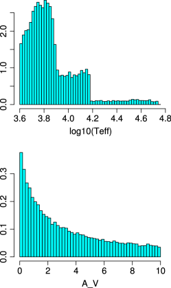
Libraries of spectra are being assembled or created for Gaia purposes. Our stellar libraries are based on the Basel (Lejeune et al. lejeune97 (1997)) and MARCS (e.g. Gustafsson et al. gustafsson08 (2008)) libraries plus an OB star library from J.-C. Bouret. Together these span the full range of effective temperature, metallicity and surface gravity. The galaxy library is described by Tsalmantza et al. tsalmantza08 (2008) (see also Tsalamantza et al. tsalmantza07 (2007)). It is based on synthetic spectra derived from galaxy evolution models with several astrophysical parameters, in particular those which describe the star formation history and the redshift. The quasar library is also synthetic, with each spectrum uniquely defined by the three parameters continuum slope, $\alpha$, emission line equivalent width, EW, and redshift, $z$ (Claeskens et al. claeskens06 (2006)). Their values are chosen at random from a distribution which is flat in redshift over the range 0–5.5, flat in $\alpha$ from $-4$ to $+3$ and exponentially decreasing in EW from 0 to 100 000 Å. We further simulated the galaxy and stellar spectra at random values of interstellar extinction over the range $A_{V}=$ 0–10 (with fixed extinction law $R_{V}=3.1$). The main stellar parameters which influence the potential contamination with the quasars are ${\rm T}_{\rm eff}$ and $A_{\rm V}$; their distribution is plotted in Fig. 1. The distributions may be a little artificial (the three “steps” reflect the three libraries), but they are sufficient for the purpose of this article.

Figure 1: The distribution of stellar parameters in the training and testing data sets

This data set is obviously rather limited (e.g. purely synthetic data, no extinction in the quasars, no emission line stars, no strong galaxy emission). Our main goal at this stage is not to produce a data set tuned to the real Gaia sky. We discuss the issue of training sets more in section 5.

3.3 Gaia simulated spectra

To build and test the processing pipeline, the DPAC has built a sophisticated data simulator (Luri et al. luri05 (2005)). For each object in the spectral libraries we simulate its BP/RP spectrum, parallax and proper motion, including all sources of random error. Gaia observes every part of the sky between 40 and 200 times over five years (depending on ecliptic latitude). The average number of spectra for an object in an end-of-mission stack is 72, which we use here. Our simulated data are the so-called cycle 3 data (Sordo & Vallenari sordo08 (2008)).

Figure 2: Random selection of five stars (blue solid lines) and five quasars (red dashed lines) (G=18.5, noise included). The first 46 pixels are the blue channel (Blue Prism, BP), the remaining 40 the red channel (Red Prism, RP), separated by a dashed line.

Figure 3: The (noise-free) library spectra for the stars (top panel) and quasars (bottom panel) shown in Fig. 2. The photon flux has been normalized in each case to have a maximum of 1.0.

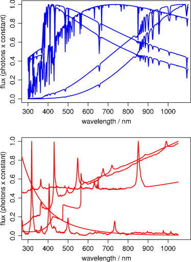
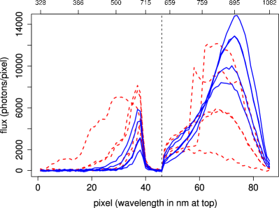
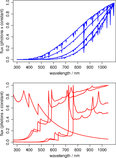
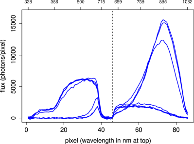
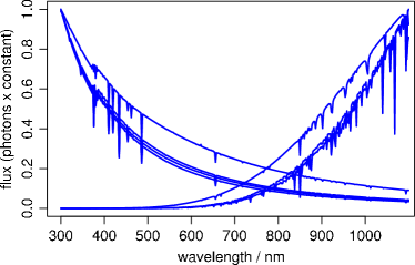
Gaia prism spectra are obtained in two channels, one for the blue called BP and one for the red called RP, with cut-offs defined by the (silver) mirror response in the blue, CCD QE in the red, and bandpass filters in the middle. After removal of low sensitivity regions, BP ranges from 338 to 998 nm over 46 pixels and RP from 646 to 1082 nm over 40 pixels. We use all 86 pixels as separate inputs to the classifier (we do not attempt to combine the wavelength overlapped region). The dispersion varies strongly with wavelength from 3 nm/pixel (blue end) to 30 nm/pixel (red end). The instrumental point spread function (PSF) is significantly broader than the pixel size, and in one conservative estimate there are are only 18 independent measures in BP/RP (Brown brown06 (2006)). Example spectra are shown in Fig. 2. The dominant noise source is Poisson noise from the source, so the SNR is approximately the square root of the flux. (At G=20, the fluxes are four times smaller and the SNR is about half.) The corresponding library spectra (i.e. prior to being put through the Gaia instrument simulator) are shown in Fig. 3. The original stellar library spectra are calculated at a resolution of 0.1 nm and show many absorption lines, so to avoid confusion, we just plot every 20^th pixel. Note how much information is lost – especially concerning the spectral lines – in BP/RP.

3.4 Simulated astrometry

Figure 4: Distribution of the simulated astrometry. Blue/solid=star, red/dashed=quasar, black/dotted=galaxy (which is indistinguishable from the quasars).

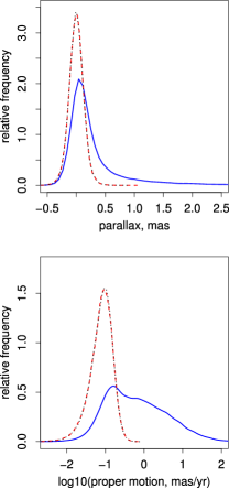
We included the astrometry in our classifiers in the expectation that it could help distingiush galactic and extragalactic objects. Fig. 4 shows the distribution of the simulated astrometry (with noise) for G=18.5. Astrometry for the extragalactic objects is just zero plus noise. Note that this causes negative parallaxes (which are preserved in the Gaia astrometric data processing for model fit assessment purposes). Stellar parallaxes, $\varpi$, are simulated in a way to ensure consistency with the apparent and absolute magniutudes and stellar parameters. The stellar proper motions are drawn at random from a zero mean Gaussian with standard deviation $10\varpi$/yr, which simiulates a distance-independent space velocity distribution with a standard deviation of 50 km/s.

At G=18.5, the Gaia parallax error is typically 0.1 mas and the proper motion error around 0.14 mas/yr (both dominated by source photon statistics). The errors are twice as large at G=20.0.

3.5 Train and test data

The input data for our classifiers is BP/RP plus astrometry (although it turns out that inclusion of astrometry hardly improves the results). Models are trained and tested on noisy data and a single G-band magnitude is used in each experiment.

Train and test data are drawn at random (without replacement) from a common data set. Unless stated otherwise, the training data set comprises 5000 objects from each of the three classes and the test data 60 000 objects of each class. The reason for the large number in the test set will become clear in section 4.3.

4 Results

4.1 Overview of the experiments and explanation of the figures

We present results for three experiments

1. objects at G=18.5,

2. as (1), but in which quasars with emission line equivalent widths less than 5000 Å have been removed from the training data set, leaving 2901 quasars (the test set is unchanged),

3. as (2), but for G=20.0.

We show results for both the “nominal” and “modified” cases. In the nominal cases, the class fractions are those given by the data sets themselves, namely $f^{train}=f^{test}=(1,1,1)$ for (star, quasar, galaxy) respectively, except for the training data in cases 2 and 3 which has $f^{train}=(1,0.58,1)$. (We list here the class fractions prior to normalization.) In the modified cases, the DSC output probabilities are modified (as described in section 2.4) to accommodate different expected class fractions (priors). Quasars are made 1000 times rarer, so $f^{mod}=(1,1/1000,1)$. This is the order of the star/quasar ratio we expect for Gaia at G=20. (In comparison, a larger ratio is found in SDSS – as high as 0.015 at $g=18.5$ depending on Galactic latitude – although this estimate probably suffers from stellar incompleteness (Bailer-Jones & Smith 2008a ).) Galaxies will also be rare, so in reality we should also modify their class fraction. Yet we intentionally modify the class fractions just for a single class here in order to better illustrate our prior modification method.

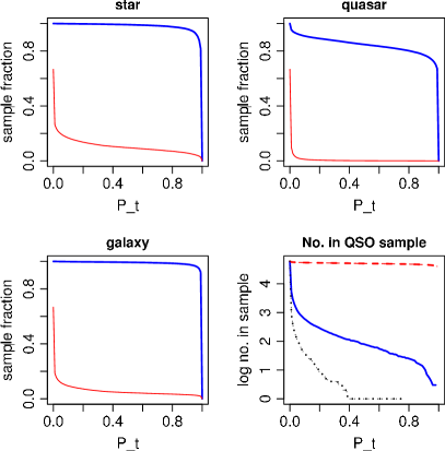
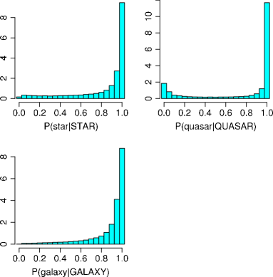
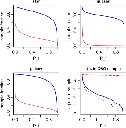
Results are presented in three ways. The first is a confusion matrix, in which an object is assigned to the class with the largest DSC output (most probable class) and the table shows the correct classifications (on-diagonal values) and misclassification values (off-diagonal values) as percentages. Second, we show histograms of the posterior probabilities. All histograms are density estimates with unit area and always show the actual test data sets (no adjustment in the number of plotted objects for the modified cases). We then set thresholds, $P_{t}$, on the posterior probabilities in order to build samples (section 2.2). The third method of illustration shows how the sample completeness and contamination varies with this threshold for each output class.

4.2 G=18.5 with all quasars in the training data

We report only briefly on this case, primarily in order to motivate the removal of the low EW quasars in experiments (2) and (3).

Table 1: Confusion matrix for class assignments from maximum probability. Each row corresponds to a true class and sums to 100%. Nominal priors, G=18.5

	galaxy	quasar	star
GALAXY	99.36	0.19	0.45
QUASAR	1.03	96.04	2.94
STAR	0.49	0.88	98.63

Figure 5: Histograms of DSC outputs for each class showing how confident DSC is of identifying each class. Nominal priors, G=18.5

Figure 6: Completeness (blue/thick line) and contamination (red/thin line) of a sample as a function of the probability threshold. The bottom right panel shows the (logarithm) of the actual number of different types of class in the quasar sample: stars (blue/solid line); quasars (red/dashed lines); galaxies (black/dotted line). Nominal priors, G=18.5

Figure 7: Completeness (blue/thick line) and contamination (red/thin line) of a sample as a function of the probability threshold. The bottom right panel shows the (logarithm) of the actual number (thick lines) of different types of class in the quasar sample (i.e. in the test set): stars (blue/solid line); quasars (red/dashed lines). The thin lines show the corresponding effective number of objects for the modified case. Modified priors, G=18.5

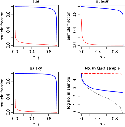
The confusion matrix (Table 1) shows that good classification accuracy is achieved with the nominal model. The histograms of the posterior probabilities (Fig. 5) further show that these classifications are achieved with high confidence. This translates into a satisfactory trade-off in sample completeness and contamination at thresholds between 0.5 and 0.9 (Fig. 6). The bottom right-hand panel shows that stars rather than galaxies are the main contaminant in the quasar sample. If we now proceed to the modified model, the C&C curves are very different (Fig. 7). While we would expect higher contamination for a given completeness level for quasars (because they are now very rare), we see that it is impossible to get a low contamination quasar sample at all. The bottom right-hand panel of that plot explains why: The effective number of stars in the sample (366) is much higher than the effective number of quasars (63), so the contamination is high, $366/(366+63)=0.85$ (To recall: the effective number is the number we would have in a data set which had the modified class fractions.)

Figure 8: Examples of low EW quasars (red/dashed lines) and those stars (blue/solid lines) which are the contaminants in the quasar sample in the modified G=18.5 model

Figure 9: The (noise-free) input spectra for the stars (top panel) and quasars (bottom panel) shown in Fig. 8. The photon flux has been normalized in each case to have a maximum of 1.0.

Inspection of the contaminants shows that they are predominantly cool, highly-reddened stars, with ${\rm T}_{\rm eff}$ between 4000 and 8000 K and $A_{\rm V}$ mostly between 8 and 10 mag. While the full stellar data set is dominated by stars in this temperature range, the extinction distribution peaks towards lower extinctions (Fig. 1), so this tendency for highly extincted contaminants is significant. Figs. 8 and 9 plot a random selection of these stellar contaminants along with a random selection of quasars with lower values of the emission line EW parameter. Note how the very broad PSF of BP/RP is smoothing out the sharp features in the quasar spectra, especially at the red of the two channels where the dispersion is lower. The narrower quasar emission lines are not resolved, and these objects look more like the smoother stellar spectra. We hypothesize that if we remove such quasars from our training set, and thus from our definition of quasars, then the SVM should not so readily confuse these stars with our quasar class. We test this in the next experiment (section 4.3).

Table 2: Model-based priors for the nominal, $P(C_{j}|\theta^{nom})$, and modified, $P(C_{j}|\theta^{mod})$, cases for the full training data and the case in which low EW quasars have been removed (“nlEW”). For comparison we show the class fractions relevant to he nominal models, $f^{train}_{i}$, and the modified models $f^{mod}_{i}$

	data	$G$	star	quasar	galaxy
$P(C_{j}|\theta^{nom})$	full	18.5	0.3380	0.3279	0.3341
$f^{train}_{i}$	full	18.5	0.3333	0.3333	0.3333
$P(C_{j}|\theta^{mod})$	full	18.5	0.4965	0.002514	0.5010
$f^{mod}_{i}$	full	18.5	0.4998	0.000500	0.4998
$P(C_{j}|\theta^{nom})$	nlEW	18.5	0.367	0.283	0.350
$P(C_{j}|\theta^{nom})$	nlEW	20.0	0.368	0.260	0.372
$f^{train}_{i}$	nlEW	both	0.388	0.225	0.388
$P(C_{j}|\theta^{mod})$	nlEW	18.5	0.4983	0.000328	0.5013
$P(C_{j}|\theta^{mod})$	nlEW	20.0	0.4762	0.000277	0.5234
$f^{mod}_{i}$	nlEW	both	0.4998	0.000500	0.4998

Table 2 lists the model-based priors (section 2.3). The first line is for the nominal model. The second row gives, for comparison, the fraction of objects in each true class, $i$, in the training data. These we may consider as frequentist estimates of the model priors, insofar as the frequency distribution of the classes dicates these. At least for this SVM model with equal class fractions, the model-based priors are close to the class fractions.

The third and fourth lines give the same but for the modified model. Now we see that the modified class fraction, $f^{mod}_{i}$, for the quasars is not a good proxy for the model-based prior. This implies that its use in equation 4 will give poor estimates for the true posterior probabilities. We could attempt to improve this by an iterative procedure: Now that we have the model-based priors, we can recalculate the model posteriors directly from Bayes’ equation (2) – rather than our approximation (equation 4) – and then recalculate the model-based priors with equation 3. However, we don’t do this because in our main experiments (next), the discrepancy is not as large.

4.3 G=18.5 with low EW quasars removed from the training data

Motivated by the results of the previous experiment, we removed the low equivalent width quasars (EW$<5000$ Å) from the training data set (2099 of 5000) and re-tuned and re-trained the SVM. (The choice of $5000$ Å is somewhat arbitrary.) The test set is unchanged.

4.3.1 The nominal model

Table 3: Confusion matrix for class assignments from maximum probability. Each row corresponds to a true class and sums to 100%. Nominal priors, G=18.5, no low EW quasars in training data

	galaxy	quasar	star
GALAXY	99.37	0.00	0.63
QUASAR	4.22	85.59	10.19
STAR	0.68	0.13	99.19

Comparing the confusion matrix (Table 3) to that in the previous experiment, we now see that fewer quasars are correctly classified, with 10% being misclassified as stars. Yet this loss of quasars is balanced by the fact that six times fewer stars are now misclassified as quasars (0.13% rather than 0.88% previously, or 78 stars rather than 528). This is what we wanted to achieve by modifying the training sample.

Note how few galaxies are misclassified as stars and quasars, and how this has hardly changed from the previous experiment. In all experiements we have performed with these data (including many not reported here), the galaxies are always classified with high confidence. As we are not changing the class fractions for galaxies – they are acting mostly to make the classification problem for the SVM harder – we focus on the stars and quasars from now on.

Figure 10: Histograms of the DSC class posterior probabilities, shown for each output class (columns) split for objects of each true class (rows). Nominal priors, G=18.5, no low EW quasars in training data

Figure 11: Completeness (blue/thick line) and contamination (red/thin line) of a sample as a function of the probability threshold. The bottom right panel shows the (logarithm) of the actual number of different types of class in the quasar sample: stars (blue/solid line); quasars (red/dashed lines); galaxies (black/dotted line). Nominal priors, G=18.5, no low EW quasars in training data

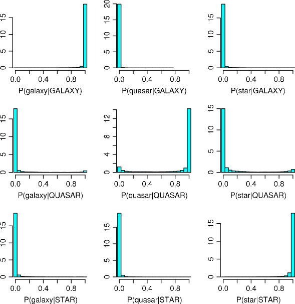
We summarze the model confidence (posterior probabilties) in the histograms in Fig. 10. We can read several things from this: the leading diagonal shows $P({\tt class}|{\tt CLASS})$, how confident the true positives are; the central row shows $P({\tt class}|{\tt QUASAR})$, the probabilities assigned to each class for true quasars; the central column shows $P({\tt quasar}|{\tt CLASS})$, the quasar probabilities assigned to objects of each true class. We see that the confidences for the correct classes are still high. However, comparing with the results of the previous experiment (Fig. 5), we now see a set of true quasars which are now assigned very low probabilities, $P({\tt quasar}|{\tt QUASAR})$. These are predominantly (but not exclusively) the low EW quasars that were removed from the training data. These low probability cases are reflected as a dip in the quasar completeness curve (Fig. 11) at low $P_{t}$. These quasars show up in the star sample and we correspondingly see a higher contamination for the stars. Yet the positive trade off from this is a lower quasar sample contamination. To give numbers: At $P_{t}=0.8$ the completeness and contamination fractions for stars are 0.976 and 0.071 respectively and for quasars are 0.8020 and 0.0005. So we see that even with the nominal model we can get a very pure quasar sample, but at the cost of a rather unpure stellar one.

4.3.2 The modified model

Figure 12: Histograms of the DSC class posterior probabilities, shown for each output class (columns) split for objects of each true class (rows). Modified priors, G=18.5, no low EW quasars in training data

Figure 13: Completeness (blue/thick line) and contamination (red/thin line) of a sample as a function of the probability threshold. The bottom right panel shows the (logarithm) of the actual number (thick lines) of different types of class in the quasar sample (i.e. in the test set): stars (blue/solid line); quasars (red/dashed lines). The thin lines show the corresponding effective number of objects for the modified case. There are no galaxy contaminants. Modified priors, G=18.5, no low EW quasars in training data

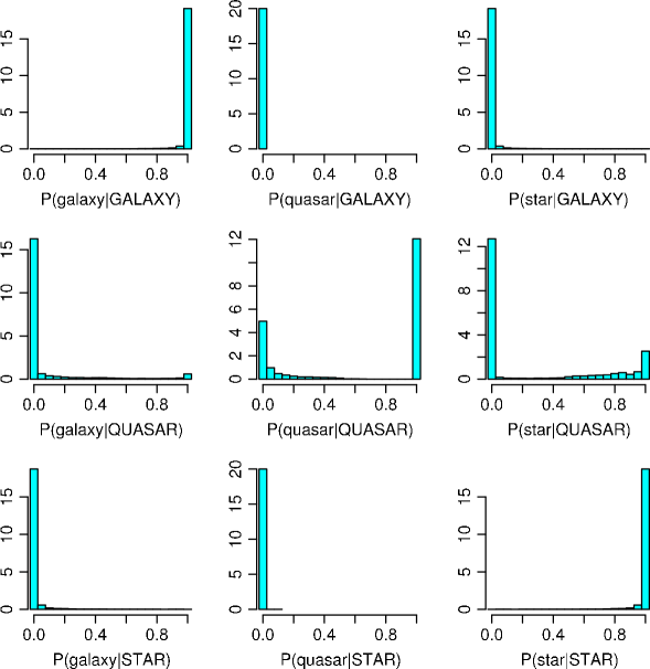
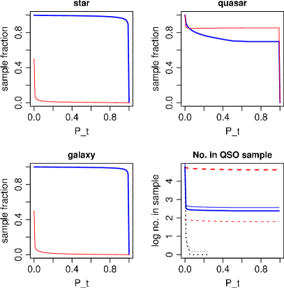
We turn now to the modified model in which our prior is that quasars are 1000 times rarer. The histograms of the posteriors are show in Fig. 12 which we may compared to the nominal case in Fig. 10. The main difference can be seen in the central plot, where we now observe a significant peak around zero probability for $P({\tt quasar}|{\tt QUASAR})$: the modified model has a high barrier to classifying anything as a quasar. This is the result of the probability remapping, equation 4 (whereby the impact of the normalization should not be ignored). This provides more discrimination between those quasars which, in the nominal case, were all assiged an output probability of almost 1.0.

Fig. 13 shows the C&C for the modified model. It is significantly different from the nominal case. The quasar completeness is slightly reduced, but we win a much lower contamination. Indeed, at $P_{t}=0.11$ the contamination drops to zero for a sample completeness of 65%. This translates to a contamination of less than 1 in $0.65\times 60000=$ 39 000. Not only is this better than for the nominal model (where the contamination only drops to zero at $P_{t}=1.0$), but now the star and galaxy contaminations are also much lower.

The bottom right-hand plot of Fig. 13 shows the actual (solid line) and effective (thin line) number of objects in the quasar sample. At $P_{t}=0.8$ these are 36149 ($=10^{4.56}$) and 54 ($=10^{1.73}$) respectively. If we had done this experiment with a test set containing, say, only 2000 quasars, then the effective number of quasars in the resultant sample would only have been $54\times(2000/60\,000)=1.8$. This is not enough to draw results of any significance and explains why we need large test sets for evaluating the modified model.

Table 4: Confusion matrix for class assignments achieved by applying a probability threshold. Each row gives the percentage of objects of each true class assigned to the different output classes (columns). As an object may now be assigned to more than one class, the values in a row no longer sum to 100%, plus some objects may remain unclassified. The thresholds applied are $P_{t}=0.2$ for quasars and $P_{t}=0.8$ for stars and galaxies. Modified priors, G=18.5

	galaxy	quasar	star	unclassified	Effective
					fraction
GALAXY	98.97	0.00	0.64	0.73	1.0
QUASAR	6.82	62.00	26.37	8.73	0.001
STAR	0.78	0.00	98.69	1.09	1.0

The confusion matrix for this modified case is shown in Table 4. As class assignments are now based on thresholds rather than maximum probability, and because we can set these thresholds independently of one another, a given object may be assigned to more than one class or it may remain unclassified. Therefore the values in a row no longer sum to 100%. Here we use thresholds of $0.8,0.2,0.8$ for galaxy, quasar and star respectively. The quasar threshold is chosen to give zero quasar contamination and delivers a good completeness of 62%. The star and galaxy threholds were also chosen from inspecting the C&C curves in Fig. 13, and yield high completeness (around 99%) and about 0.7% cross contamination. From a first glance at the table we might think that this star sample is heavily contaminated by quasars (26.37%). Yet we must remember that quasars are effectively rare, so the fraction of quasar contaminants expressed as percentage of objects in the star output is

$$100\%\times\frac{26.37\times 0.001}{26.37\times 0.001+98.69\times 1.0+0.64\times 1.0}=0.03\%$$

(The quasar contamination of the galaxy sample is even smaller). Recall also that the histograms, such as Fig. 12, show the actual number of objects in the test set, not the effective number. So what looks like a relatively large number of quasars confidently classified as stars corresponds to a far smaller number in the target population.

Figure 14: Spectra of stars which are most confused as quasars, namely those 7 stars which have the highest values of $P^{mod}({\tt quasar}|{\tt STAR})$. G=18.5, modified priors, no low EW quasars in training data.

Figure 15: The (noise-free) input spectra for the stars shown in Fig. 14. The photon flux has been normalized in each case to have a maximum of 1.0.

It is again interesting to identify the misclassifications. Those true stars which are most confused as quasars are show in Fig. 14. As can be seen from the plot of the corresponding library spectra (Fig. 15), four of these are hot stars with ${\rm T}_{\rm eff}$ $\simeq$ 40 000 K. The other three are cooler (two around 4000 K, one around 7000 K) but have very high extinctions (8–9 magnitudes $A_{\rm V}$). This gives rise to the much larger flux in the red which DSC confuses with a quasar-like broad emission line feature.

We recall that in this experiment we removed the low EW quasars from the training set, but not the test set. We may, therefore, expect this model to perform particularly badly on these objects. However, if we plot Fig. 12 just for these objects it turns out to be broadly similar, although with about half as many objects in the $P({\tt quasar}|{\tt lowEWQUASAR})=1$ bin and twice as many in the $P({\tt quasar}|{\tt lowEWQUASAR})=0$ bin. So while this model doesn’t do as well on the objects omitted from the training data, it is still able to assign many a high probability. That is, DSC has been able to extend its recognition of quasars to lower EW cases than it was trained on.

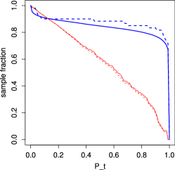
4.3.3 Testing the predictions of the modified model

Figure 16: Comparison of the completeness (blue/thick lines) and contamination (red/thin lines) obtained with the modified model at G=18.5 (no low EW quasars in training data). The solid lines are the predictions (same as those in the the top right panel of Fig. 13) and the dashed lines are the measurements from a data set in which quasars really are rare (class fractions of (1,1/1000,1))

The C&C plots for the modified model are of course just predictions of what the C&C would be if we applied the modified model to a real data set which has the modified population fractions. We can test these predictions by building a new test data set in which the population fractions really are (1,1/1000,1). To do this we took the original test data set but retained just a random selection of 1/1000 of the quasars (i.e. 60 quasars). We applied the modified model and calculated the C&C (now using equation 1 of course, not equation 5). As there are only 60 quasars in this set, the predictions have high variance, so we bootstrapped the selection 20 times. Fig. 16 shows that the measured C&C are very close to the predictions, thus validating our approach.

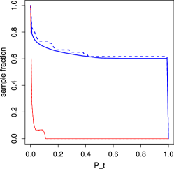
4.3.4 The nominal model yields high contamination when quasars are rare

Figure 17: As Fig. 16 but now for the nominal model

Theoretical arguments aside, could we nonetheless use the nominal model to classify data sets in which quasars are rare? To assess this, we applied the nominal model to the few-quasar data set from the above test (section 4.3.3). The measured C&C are plotted in Fig. 17 as the dashed lines. These agree well with the C&C we would predict on the effective test data set (i.e. using equation 5) but using the nominal model, which are shown as the solid lines in Fig. 17. While they agree, this figure shows that the sample contamination is far higher when using the nominal model than the modified model (Cf. Fig. 16). That is, the modified model is superior at obtaining pure quasar samples. This demonstrates that we must take into account the expected class fractions (i.e. use a suitable prior) when applying a classifier to a data set in which we expect a class to be rare.

Finally for this experiment, we note that the model-based priors agree quite well with the training data class fraction or the modified class fraction for the nominal and modified models respectively (Table 2).

4.4 G=20.0 with low EW quasars removed from the training data

Table 5: Confusion matrix for class assignments from maximum probability. Each row corresponds to a true class and sums to 100%. Nominal priors, G=20.0, no low EW quasars in training data

	galaxy	quasar	star
GALAXY	93.53	0.12	6.66
QUASAR	7.40	77.13	15.47
STAR	13.92	0.21	85.87

Figure 18: Histograms of DSC outputs for each class showing how confident DSC is of identifying each class. Nominal priors, G=20.0, no low EW quasars in training data

Figure 19: Completeness (blue/thick line) and contamination (red/thin line) of a sample as a function of the probability threshold. The bottom right panel shows the (logarithm) of the actual number (thick lines) of different types of class in the quasar sample (i.e. in the test set): stars (blue/solid line); quasars (red/dashed lines). Nominal priors, G=20.0, no low EW quasars in training data

Figure 20: Completeness (blue/thick line) and contamination (red/thin line) of a sample as a function of the probability threshold. The bottom right panel shows the (logarithm) of the actual number (thick lines) of different types of class in the quasar sample (i.e. in the test set): stars (blue/solid line); quasars (red/dashed lines). The thin lines show the corresponding effective number of objects for the modified case. There are no galaxy contaminants. Modified priors, G=20.0, no low EW quasars in training data

At G=20 the noise is higher, so we expect DSC to perform less well. The basic class assignment based on maximum posterior class probability is indeed worse (Table 5). Comparing with Table 3 we see that the stars suffer in particular, with only 86% being correctly classified, as opposed to 99% at G=18.5. This is reflected by the lower confidence the model gives to its classifications (Fig. 18). Likewise, the completeness is lower and the contamination higher at a given threshold (Fig. 19).

If we now modify the priors and recalculate the posterior probabilities then we see a similar shift in the distributions that we did for the G=18.5 case (histograms not shown). The C&C plot with the modified model is shown in Fig. 20. What stands out immediately is that we are still able to get a clean (zero contamination) quasar sample. This occurs once $P_{t}=0.07$, at which point the completeness is 58% (and remains at above 50% if we choose to take a larger threshold). This compares to a completeness of 65% at $P_{t}=0.11$ for zero contamination at $G=18.5$. Thus we see that the higher noise in the data can be translated into a lower completeness (which is acceptable) rather than a raised contamination (which is not). Notice that there is no guarantee that the contamination should drop to zero before $P_{t}=1$ (cf. section 4.2), so this is an important result.

4.5 The impact of using astrometry in classification

We may expect parallaxes and proper motions to provide a good discriminant between Galactic and extragalactic objects. Yet it turns out that if we remove astrometry from the DSC, the performance hardly degrades (accuracy decreases by no more than 1%). This observation may not be surprising, because the majority of objects with astrometry consistent with zero (within the measurement errors) are actually stars, and that is because our training sample is dominated by distant stars. It is also not specific to the SVM. We also built a two-stage classifier, in which (1) an SVM predicts classes based only on photometry and (2) Gaussian mixtures are used to model the density in the 2D astrometric space and predict classes. The probabilities are then combined to give a single posterior (Bailer-Jones & Smith 2008b ). The results are no better than an SVM using BP/RP and astrometry (although the two-stage classifier offers more flexibility and interpretability).

4.6 The effect of reducing the fraction of quasars in the training data

In section 2.3.2 we argued that the model class priors are not necessarily dictated by the class fractions in the training data. Moreover, in attempting to match the training data distribution to that in the target population for a rare object, we may end up with very few objects in the training data, such that the classifier does not learn to classify them well.

Figure 21: Quasar sample completeness (thick blue line) and contamination from stars (thin red line) and galaxies (dotted black line) as a function of varying the fraction of quasars in the training data set (the first two values are 0.1% and 1%)

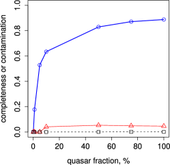
We test this by varying the fraction of quasars in the training data set, $q$, from 100% (equal class fractions) down to 0.1% (60 quasars). We then build samples based on maximum probability and measure the C&C (again using equation 5 to account for the modified class fractions). Fig. 21 shows how the completeness and contamination of the quasar sample varies with $q$. For modest reductions in $q$ the contamination is 5%, which is too high for a pure sample (although the samples are built using maximum probability, so we could reduce this at the cost of reduced completeness). Surprisingly, the contamination actually drops to zero once the quasar fraction drops below 5%. However, this comes at the price of greatly reduced completeness of just 0.1% at $q=$ 0.1%. This we can directly compare to the results from the modified model in experiment (2) (section 4.3.2), where the completeness is still 62%. Thus we conclude that pruning the training data set is not the way to achieve a good classifier for a rare class.

5 Discussion

5.1 Training data distributions and class definitions

Any supervised method is limited by the data it is trained on. Systematic differences between these and the target population can compromise the classifier. It is not the goal of this article to present the final classifier for Gaia, so we have not yet optmized the training sets. Nonetheless, our work does raise some issues relevant to this important next step, which we briefly discuss.

First, we found that removing the low EW quasars was important for achieving clean quasar samples in the modified case. This may reflect a limitation of the SVMs, but it raises the general issue of how to set the training data distribution. We do not expect a supervised method to perform well on regions of the data space not included in the training data (although we did find that the model could correctly classify many low EW quasars). For this reason, DSC will be preceeded by an “outlier detector” in the classification pipeline. This assesses how well an observed object is “covered” by the training space and only passes “known” objects to DSC. It could be based on density estimation (in low dimensions) or one-class SVMs.

Second, if we are building a classifier only to look for a specific type of object, then we don’t need to aim for completeness in the training sample (although we do need to include potential contaminants). For example, none of our quasar simulations include interstellar extinction (unlike the stars and galaxies). This could be motivated by saying we do not trust extinction laws and just want to find unreddened quasars. We are free to make this choice at the cost of reduced completeness of real quasars. If we included reddened quasars in the test set, then either they would be classified as quasars anyway (in which case the completeness goes up), or they would be classified as something else. Either way, the quasar contamination would not increase so our conclusion about building pure samples of unreddened quasars is unaffected. Incidentally, the results in section 4 are very similar if we repeat the experiments but now with interstellar extinction applied also to the quasars. The main difference is that the quasar sample completeness is reduced by around 10%, with the more reddened quasars now contaminating the star samples. The quasar contamination is not increased.

Third, how should we define the classes? If we had split the quasars into two classes (e.g. high and low emission line EW) maybe this would help the SVM to retain zero contamination on the high EW class without having to remove the low EW quasars entirely from the training data. This will be the subject of future work.

Gaia does not exist in a void; we of course have information from other catalogues/surveys to help us identify quasars. The full DSC is actually a multi-stage algorithm, in which the present paper just describes the stage based on the BP/RP spectrum. Other stages provide class probabilities based on other data, for example the source magnitude or Galactic latitute or external catalogues, in which case we might call them “priors”. We will describe this multi-stage approach in a future paper.

5.2 How do we interpret posterior probabilities?

When we build a sample by applying a threshold, all of the objects have a posterior probability which is at least as high as the threshold. For example, with the modified model in section 4.3.2, we were able to set $P_{t}=0.11$ and produce a sample of only quasars. There is of course no guarantee that all samples built using this threshold have no contaminants. On the other hand, this threshold is not a statement about the sample as a whole: it would be wrong to expect only 11% of the sample to be quasars. We need to look at the actual proabilities, not a lower limit. How can we use these? Imagine a case in which we set $P_{t}=0.90$ and thereby obtained a sample of 1000 (supposed) quasars, all which happen to have $P({\tt quasar})=0.95$. We would reasonably expect 5% not to be quasars. Yet we must be careful with such an inference, because posterior probabilities are not frequencies (especially if we have very non-uniform priors, e.g. class fractions of $(1,0.001,1)$).

Figure 22: The left panel shows the variation with $r$ of $P(n=1000,r,p=0.95)$ (equation 7), the probability that there are exactly $r$ contaminants in the quasar sample of $n$ objects, each with posterior quasar probability of $p$. The right hand panel is 1 minus the cumulation of this (equation 8), and so shows the probability that there will be more than $r$ contaminants (shown as the contamination fraction $r/n$).

How can we make statements about the sample as a whole from the individual probabilities? The general case is complex, but for the case that all the probabilities are the same, the solution is simple. If $P({\tt quasar})=p$ for all objects in a sample of size $n$, then the probability that exactly $r$ of them ($r\leq n$) are non-quasars is

$$P(n,r,p)=\frac{n!}{r!(n-r)!}(1-p)^{r}p^{(n-r)}$$ (7)

The left panel of Fig. 22 shows how (the logarithm of) this quantity varies with $r$ for $n=1000$ and $p=0.95$. (It has a maximum of $P(n,r,p)=0.058$ at $r=50$). By summing equation 7 over ranges of $r$ we can make more useful statements. For example, summing from $r=0$ to $r=50$, we can say that the probability that there are 50/1000=5% contaminants or fewer is 0.54. Equivalently, the probability that there is more than 5% contamination is 0.46. The right hand panel of Fig. 22 shows this for variable $r$. Specifically it plots

$$1-\sum_{r^{\prime}=0}^{r^{\prime}=r}P(n,r^{\prime},p)$$ (8)

against $r/n$, the contamination fraction. This figure agrees approximately with our intuition of a 5% contamination when all posterior probabilities are 95%.

We can apply this to the case in section 4.3.3, where we applied the modified model to a test with 60 quasars. Setting $P_{t}=0.2$ we achieved a zero contamination sample of 37 quasars (62% completeness; Table 4). If we didn’t know the true classes, would we have expected zero contamination with the above calculation? The posterior probabilities are not equal (the expected distribution is $P({\tt quasar}|{\tt QUASAR})$ in Fig. 10), but we approximate by setting $p$ equal to the average for this sample, which is 0.95. Equation 8 tells us ($n=37$, $r=1$, $p=0.95$) that the probability of having one or more contaminants is 0.56. This is consistent with having no contaminants. Of course, this average probability is not very representative, so this doesn’t strictly apply. For example, we could also have taken a threshold of $P_{t}=0.50$ and still had a zero contamination sample, but in this case the average is $p=0.997$ and the probability of one or more contaminants is just 0.006.

Despite these approximations, it appears that the inferences about the sample as a whole are consistent with the individual posterior probabilities.

5.3 Why we should prefer the modified model

Ultimately we would like to know whether the modified model is “better” than the nominal one. If we ignored the issue of priors and class fractions, then our predictions of sample completeness and contamination would always be given by Fig. 11 (at G=18.5), regardless of the true class fractions in the target population. If we improve this by instead using equation 5 to accommodate the modified class fractions (but still with the nominal model posteriors), then our predictions would be the solid lines in Fig. 17. Yet both are poor predictions of the actual completeness and contamination in a sample where quasars are rare (dashed lines in Fig. 16).

We demonstrated (in section 4.3.4) that the application of the nominal model to a data set with rare quasars gives poorer results (larger contamination) than the modified model at a given probability threshold. It is not yet clear whether we could just use the nominal model but with much higher probability thresholds to achieve similar results. However, there are two reasons why we should not want to do this. First, as we must not build test data sets with very small numbers of the rare class, we would still have to use the modified class fractions in order to correctly predict the C&C (section 2.5). Second, we want models which deliver actual probabilities, not just numbers between 0.0 and 1.0 to which we apply a meaningless threshold. This is especially important if we later want to update the probabilities, e.g. in a multi-stage classifier. We therefore believe it is better to use the modified model.

6 Conclusions

We have introduced a method of probability modification which can be used to build clean samples of rare objects for which the completeness and contamination can be reliably predicted. We have demonstrated this using a support vector machine classifier, although it may, of course, be used in conjunction with any classifier which gives probabilities. The main conclusions of our work are as follows.

• To construct a pure sample of objects we should use a probabilistic classifier and only select objects with high probabilities. By varying this probability threshold we can trade off sample completeness and contamination.

• To achieve pure samples of rare objects, we must take into account the expected class fractions in the target population, which act as a prior probability on the classifier. We use these to modify the nominal classifier outputs to give the modified model.

• We applied our modified model to a three class problem in which quasars are simulated to be 1000 times rarer than stars and galaxies. We can achieve a pure quasar sample (zero contamination) yet still reach a sample completeness of 50–65% for magnitudes down to G=20.0. Although the test set is finite in size, this correponds to an upper limit in the contamination of 1 in 39 000. This is more than adequate for establishing an astrometric reference frame for Gaia: If Gaia observes half a million quasars, we can build a quasar sample of 250 000 with no more than 13 contaminants.

• While achieving this pure quasar sample, we simultanesouly achieve very complete galaxy and star samples (both 99%) with low contamination (both 0.7%) (figures for G=18.5).

• These results were achieved after removing quasars with low equivalent width emission lines from the training sample (defined somewhat arbitrarily as 5000 Å). Including these precluded establishing a low contamination sample, because it resulted in cool (4000–8000 K) highly reddened ($A_{\rm V}$ = 8–10) stars being confused with them. After removing these quasars, the first stars to contaminate a quasar sample (if we set a low threshold) are these reddened cool stars as well as hot stars (${\rm T}_{\rm eff}$ $>$ 40 000 K).

• Including parallax and proper motion (either as additional SVM inputs, or in a separate mixture model classifier) hardly changes the performance. This is not surprising since the majority of objects with astrometry consistent with zero are actually stars.

• Extending the training and testing sets to include quasars with a full range of interstellar extinction does not significantly alter the results (completeness slightly lower, but contamination unaffected)

• All classification models have a prior, but the prior is often not explicit and are sometimes implicitly influenced by the training data distribution. We have introduced a simple method for calculating the implicit priors in a classification model, which we call the model-based priors. In many cases we have experimented with, these priors are close to the true class fractions in the training data (nominal model) or modified class fractions (modified model).

• We recommend that a classifier be trained on roughly equal numbers of objects in each class so that it can properly learn the class distributions or boundaries. By determining the model-based priors and replacing them with something more appropriate to the target population (e.g. quasars being rare), we can produce a modified model with superior performance. In particular, this is far better at producing large, pure samples of the rare class.

• With our approach we can apply the model to any new target population by specifying the appropriate class fractions (priors) without having to change the training data distribution or re-train the model.