Phase-space structures in quantum-plasma wave turbulence

Abstract

The quasilinear theory of the Wigner-Poisson system in one spatial dimension is examined. Conservation laws and properties of the stationary solutions are determined. Quantum effects are shown to manifest themselves in transient periodic oscillations of the averaged Wigner function in velocity space. The quantum quasilinear theory is checked against numerical simulations of the bump-on-tail and the two-stream instabilities. The predicted wavelength of the oscillations in velocity space agrees well with the numerical results.

I Introduction

Quantum plasmas have attracted a renewed attention in recent years. The inclusion of quantum terms in the plasma fluid equations – such as quantum diffraction effects, modified equations of state h1 ; m1 , and spin degrees of freedom bm – leads to a variety of new physical phenomena. Recent advances include linear and nonlinear quantum ion-acoustic waves in a dense magnetized electron-positron-ion plasma Khan , the formation of vortices in quantum plasmas Haque , the quantum Weibel and filamentation instabilities h2 –Bret , the structure of weak shocks in quantum plasmas Bychkov , the nonlinear theory of a quantum diode in a dense quantum magnetoplasma b , quantum ion-acoustic waves in single-walled carbon nanotubes Weiw , the many-electron dynamics in nanometric devices such as quantum wells MH1 ; MH2 , the parametric study of nonlinear electrostatic waves in two-dimensional quantum dusty plasmas Ali , stimulated scattering instabilities of electromagnetic waves in an ultracold quantum plasma s , and the propagation of waves and instabilities in quantum plasmas with spin and magnetization effects s1 ; s2 .

However, to date, only few works have investigated the important question of quantum plasma turbulence. The most notable exception is the paper by Shaikh and Shukla Shaikh , where simulations of the two- and three-dimensional coupled Schrödinger and Poisson equations – with parameters representative of the next-generation laser-solid interaction experiments, as well as of dense astrophysical objects – were carried out. In that work, new aspects of the dual cascade in two-dimensional electron plasma wave turbulence at nanometric scales were identified. Nevertheless, the quantum-plasma wave turbulence remains a largely unexplored field of research. A reasonable strategy to attack these problems would consist in extending well-known techniques issued from the theory of classical plasma turbulence in order to include quantum effects.

In this context, the simplest approach is given by the weak turbulence kinetic equations first derived in Refs. Vedenov1 –Drummond1 , the so-called quasilinear theory. In quasilinear theory, the non-oscillating part of the distribution function is flattened in the resonant region of velocity space. It is interesting to carry over the basic techniques of the classical quasilinear theory to the kinetic models of quantum plasmas. The resulting quantum quasilinear equations would be a useful tool for the study of quantum plasma (weak) turbulence, and for quantum plasmas in general. In this regard, it is natural to initially restrict the analysis to the quasilinear relaxation of a one-dimensional quantum plasma in the electrostatic approximation.

Some earlier works explored the similarities between the classical plasma and the quantum-mechanical treatment of a radiation field Pines –Wei . In those papers, one of the aims was to obtain information on the classical plasma through a quantum-mechanical language. For instance, the relaxation of an instability can be viewed as the spontaneous emission of “quanta” of a radiation field described by some quasilinear-type equations. However, the application of the quasilinear method to a truly quantum plasma governed by the Wigner-Poisson system (i.e. the quantum analogue of the Vlasov-Poisson system) seems to be restricted to the work of Vedenov Vedenov . Surprisingly, there has been no systematic analysis of the consequences of the quasilinear theory in the Wigner-Poisson case. The present work is a first attempt in this direction.

This manuscript is organized in the following fashion. In Sect. 2, the quantum quasilinear equations are derived from the Wigner-Poisson system. In comparison with the classical quasilinear equations, the quantum model exhibits a finite-difference structure. The basic properties of the quantum quasilinear theory are discussed in Sect. 3, where we derive some conservation laws, as well as an appropriate H-theorem for the quasilinear equations. The existence of an entropy-like quantity is used to prove that the averaged Wigner function relaxes to a plateau, just like in the classical case. However, the distinctive feature of the quantum quasilinear equations is the existence of a transient periodic structure in velocity space, as shown in Sect. 4. In Sect. 5, the theory is checked against numerical simulations of the bump-on-tail and two-stream instabilities, with good agreement with the predictions. Conclusions are drawn in Sect. 6.

II Quantum quasilinear equations

The quasilinear equations for the Wigner-Poisson system were derived long ago by Vedenov Vedenov , without fully exploring their consequences. For completeness, the derivation procedure is reproduced here. The Wigner equation reads

$$\frac{\partial{f}}{\partial{t}}+v\frac{\partial{f}}{\partial{x}}=\int dv^{\prime}K(v-v^{\prime},x,t)f(x,v^{\prime},t)\,,$$ (1)

where

$$K(v-v^{\prime},x,t)=-\frac{iem}{2\pi\hbar^{2}}\int d\lambda\,e^{im(v-v^{\prime})\lambda/\hbar}\left[\phi(x+\lambda/2,t)-\phi(x-\lambda/2,t)\right]\,.$$ (2)

Here, $f(x,v,t)$ is the Wigner pseudo-distribution in one spatial dimension, with position $x$, velocity $v$, and time $t$. Also, $\hbar=h/2\pi$ is the scaled Planck’s constant, $e$ is the absolute value of the electron charge, and $m$ is the electron mass. The electrostatic potential $\phi(x,t)$ satisfies the Poisson equation,

$$\frac{\partial^{2}\phi}{\partial x^{2}}=\frac{e}{\varepsilon_{0}}\left(\int dvf-n_{0}\right)\,,$$ (3)

where $\varepsilon_{0}$ is the vacuum permittivity and $n_{0}$ a fixed, neutralizing ionic background. Periodic boundary conditions are assumed, with periodicity length $L$. Accordingly, for any quantity $A=A(x,v,t)$, the spatial average is

$$\langle A(x,v,t)\rangle=\frac{1}{L}\int_{-L/2}^{L/2}dxA(x,v,t)\,.$$ (4)

In particular, it is useful to define $F(v,t)=\langle f(x,v,t)\rangle$ and to restrict to $\langle\phi(x,t)\rangle=0$.

The quasilinear theory proposes a perturbation solution of the form

$$f=F(v,t)+f_{1}(x,v,t)\,,\quad\phi=\phi_{1}(x,t)\,,$$ (5)

for small $f_{1}$ and $\phi_{1}$. After averaging the Wigner equation, taking into account that $\langle\phi_{1}(x,t)\rangle=0$, we obtain from (1)

$$\frac{\partial F}{\partial t}=\frac{iem}{2\pi\hbar^{2}}\int d\lambda dv^{\prime}e^{im(v-v^{\prime})\lambda/\hbar}\left\langle\left[\phi_{1}\Bigl{(}x-\frac{\lambda}{2},t\Bigr{)}-\phi_{1}\Bigl{(}x+\frac{\lambda}{2},t\Bigr{)}\right]f_{1}(x,v^{\prime},t)\right\rangle\,.$$ (6)

In the quasilinear theory, the right-hand side of Eq. (6) is evaluated using the results of the linear theory. This implies, in particular, that the mode coupling effects are not taken into account. Notice that $F$ changes slowly, since $\partial F/\partial t$ is a second order quantity. Thus, for too strong damping or instability, the quasilinear theory is no longer valid. Also, the trapping effect can be included only in the framework of a fully nonlinear theory. Generally speaking, the conditions of validity of the quasilinear theory are still the subject of hot debates at the classical level laval .

We now introduce the spatial Fourier transforms

$$\hat{f}_{1k}(v,t) = \frac{1}{\sqrt{2\pi}}\int_{-L/2}^{L/2}dx\,e^{-ikx}f_{1}(x,v,t)\,,$$ (7)

$$\hat{\phi}_{1k}(t) = \frac{1}{\sqrt{2\pi}}\int_{-L/2}^{L/2}dx\,e^{-ikx}\,\phi_{1}(x,t)\,,$$ (8)

with the corresponding inverse transforms

$$f_{1}(x,v,t) = \frac{\sqrt{2\pi}}{L}\sum_{k}e^{ikx}\hat{f}_{1k}(v,t)\,,$$ (9)

$$\phi_{1}(x,t) = \frac{\sqrt{2\pi}}{L}\sum_{k}e^{ikx}\hat{\phi}_{1k}(t)\,,$$ (10)

where $k=2\pi n/L$, $n=0,\pm 1,\pm 2,...$ Linearizing the Wigner equation, Fourier transforming it in space and Laplace transforming it in time, we obtain

$$\hat{f}_{1k}(v,t)=\frac{em\hat{\phi}_{1k}(t)}{2\pi\hbar^{2}(\omega_{k}-kv)}\int d\lambda\,dv^{\prime}\,e^{im(v-v^{\prime})\lambda/\hbar}(e^{ik\lambda/2}-e^{-ik\lambda/2})\,F(v^{\prime},t)\,.$$ (11)

In Eq. (11), since we are interested only in the long-lived collective oscillations, the initial perturbation $f_{1}(x,v,0)$ was neglected. Finally, $\omega_{k}$ stands for the allowable frequency modes, obtained from the the well-known Drummond quantum dispersion relation

$$D(k,\omega)=1-\frac{\omega_{p}^{2}}{n_{0}}\int_{{\cal L}}dv\,\frac{F(v)}{(\omega_{k}-kv)^{2}-\hbar^{2}k^{4}/4m^{2}}=0\,,$$ (12)

which is assumed to be adiabatically valid, where ${\cal L}$ denotes the Landau contour, and $\omega_{p}=(n_{0}e^{2}/m\varepsilon_{0})^{1/2}$ is the electron plasma frequency; for brevity, we omit to write out the second argument $t$ of $F$ from here and onward.

Since $f_{1}$ and $\phi_{1}$ are real, we have the parity properties

$$\hat{f}_{1,-k}(v,t)=\hat{f}_{1k}^{*}(v,t)\,,\quad\hat{\phi}_{1,-k}(t)=\hat{\phi}_{1k}^{*}(t)\,,\quad\omega_{-k}=-\omega^{*}_{k}\,,$$ (13)

which will be used in the remainder of this paper. By defining

$$\omega_{k}=\Omega_{k}+i\gamma_{k}\,,$$ (14)

where $\Omega_{k}$ and $\gamma_{k}$ are real, the following properties also hold

$$\Omega_{-k}=-\Omega_{k}\,,\quad\gamma_{-k}=\gamma_{k}\,.$$ (15)

By using Eqs. (11) and (13) into (6), and carrying out straightforward calculations, we obtain

$$\frac{\partial F}{\partial t}=\frac{2\pi ie^{2}}{L^{2}\hbar^{2}}\sum_{k\neq 0}|\hat{\phi}_{1k}(t)|^{2}\,\left[\frac{F(v+\hbar k/m)-F(v)}{\omega_{k}-kv-\hbar k^{2}/2m}+\frac{F(v-\hbar k/m)-F(v)}{\omega_{k}-kv+\hbar k^{2}/2m}\right]\,.$$ (16)

Equation (16) can be put in a convenient form by using the parity properties (13)–(15) and that $|\gamma_{k}|$ is small so that $\gamma_{k}/[(\Omega_{k}-kv\pm\hbar k^{2}/2m)^{2}+\gamma_{k}^{2}]\simeq\pi\delta(\Omega_{k}-kv\pm\hbar k^{2}/2m)$, where $\delta$ is Dirac’s delta function. Hence we express Eq. (16) as

$$\frac{\partial F}{\partial t} = \frac{4\pi^{2}m\omega_{p}^{2}}{n_{0}L\hbar^{2}}\sum_{k>0}\frac{\hat{\varepsilon}_{k}(t)}{k^{2}}\Bigl{\{}\Bigl{[}F\Bigl{(}v+\frac{\hbar k}{m}\Bigr{)}-F(v)\Bigr{]}\delta\Bigl{(}\Omega_{k}-kv-\frac{\hbar k^{2}}{2m}\Bigr{)}$$ (17)

$$+ \Bigl{[}F\Bigl{(}v-\frac{\hbar k}{m}\Bigr{)}-F(v)\Bigr{]}\delta\Bigl{(}\Omega_{k}-kv+\frac{\hbar k^{2}}{2m}\Bigr{)}\Bigr{\}}\,,$$

in which the growth rate does not appear explicitly, and where we have defined the spectral density of the electrostatic field fluctuations as

$$\hat{\varepsilon}_{k}(t)=\frac{\varepsilon_{0}}{L}k^{2}|\hat{\phi}_{1k}(t)|^{2}\,.$$ (18)

The presence of the delta functions in Eq. (17) emphasizes the fact that only particles satisfying the resonance condition $\Omega_{k}-kv\pm\hbar k^{2}/2m=0$ are taken into account, whereas $F(v,t)$ remains unchanged in the non-resonant region of velocity space.

The time variation of the spectral density is given in the same way as in the Vlasov-Poisson case, i.e.

$$\frac{\partial\hat{\varepsilon}_{k}}{\partial t}=2\gamma_{k}\hat{\varepsilon}_{k}\,.$$ (19)

Equations (17) and (19) are the quasilinear equations for the Wigner-Poisson system. In the formal classical limit $\hbar\rightarrow 0$, they reduce to the well-known quasilinear equations for the Vlasov-Poisson system.

III Properties of the quantum quasilinear equations

Taking velocity moments of Eq. (17), several conservation laws can be easily derived. For instance, we obtain the conservation of the number of particles,

$$\frac{d}{dt}\int\,dv\,F=0\,,$$ (20)

and of the linear momentum

$$\frac{d}{dt}\int\,dv\,mv\,F=0\,,$$ (21)

where the dispersion relation (12) and the parity properties of the spectral density have been used. In addition, the total energy is also invariant

$$\frac{d}{dt}\left(\int\,dv\,\frac{mv^{2}}{2}\,F+\frac{2\pi}{L}\sum_{k}\hat{\varepsilon}_{k}\right)=0\,.$$ (22)

Intermediate steps to derive Eq. (22) require the use of the parity properties as well as the second quasilinear equation (19). In addition, a useful approximation is to consider $\Omega_{k}\simeq\omega_{p}$ for $k>0$, jointly with

$$\gamma_{k}\simeq\frac{\pi m\omega_{p}^{3}}{2n_{0}\hbar k^{3}}\left[F\left(\frac{\omega_{p}}{k}+\frac{\hbar k}{2m}\right)-F\left(\frac{\omega_{p}}{k}-\frac{\hbar k}{2m}\right)\right]\,.$$ (23)

In order to gain insight into the asymptotic behavior of $F(v,t)$, it is interesting to look for an entropy-like quantity. Following Ref. manfredi , we consider the quantity $\int F^{2}dv$, which, from Eq. (17), can be proved to obey the equation

$$\frac{d}{dt}\int dvF^{2}=-\frac{8\pi^{2}m\omega_{p}^{2}}{n_{0}L\hbar^{2}}\sum_{k>0}\frac{\hat{\varepsilon}_{k}(t)}{k^{3}}\left[F\left(\frac{\Omega_{k}}{k}+\frac{\hbar k}{2m}\right)-F\left(\frac{\Omega_{k}}{k}-\frac{\hbar k}{2m}\right)\right]^{2}\leq 0\,,$$ (24)

where the last inequality follows since all terms in the right-hand side are non-positive. This result constitutes a sort of H-theorem for the averaged distribution function.

The time derivative of the non-negative quantity in the left-hand side of Eq. (24) is always non-positive, so that asymptotically we have $\frac{d}{dt}\int dvF^{2}\to 0$, and

$$F\left(\frac{\Omega_{k}}{k}+\frac{\hbar k}{2m}\right)-F\left(\frac{\Omega_{k}}{k}-\frac{\hbar k}{2m}\right)=0\,,$$ (25)

for all wavenumbers where the spectral density is non-zero. Equation (25) also resembles the basic equation obtained when applying the Nyquist method to the stability analysis of the Wigner-Poisson system nyquist .

Equation (25) is a finite-difference-like version of the classical plateau condition [$F^{\prime}(v)=0$] in the region where the spectral density is not zero. The finite-difference structure of Eq. (25) favors the appearance of oscillations in velocity space, which are not present in the classical case. These oscillations are analyzed in detail in the next section.

IV Transient quantum oscillations in velocity space

In the derivation at the end of Sect. 3, it was implicitly assumed that the spectral density is not zero in a broad region of momentum space. In contrast, let us see what happens in the idealized situation where the spectral density $\hat{\varepsilon}_{k}$ is strongly peaked at a single mode $K$. Denoting the associated spectral density by $\hat{\varepsilon}(t)$ and using the growth rate (23), the quantum quasilinear equations read

$$\frac{\partial F}{\partial t} = \frac{mL\omega_{p}^{2}}{n_{0}\hbar^{2}}\,\hat{\varepsilon}(t)\Bigl{\{}\Bigl{[}F\Bigl{(}v+\frac{\hbar K}{m}\Bigr{)}-F(v)\Bigr{]}\delta\Bigl{(}\omega_{p}-Kv-\frac{\hbar K^{2}}{2m}\Bigr{)}$$

$$+ \Bigl{[}F\Bigl{(}v-\frac{\hbar K}{m}\Bigr{)}-F(v)\Bigr{]}\delta\Bigl{(}\omega_{p}-Kv+\frac{\hbar K^{2}}{2m}\Bigr{)}\Bigr{\}}\,,$$

and

$$\frac{d\hat{\varepsilon}(t)}{dt}=\frac{\pi m\omega_{p}^{3}}{n_{0}\hbar K^{3}}\,\hat{\varepsilon}(t)\left[F\left(\frac{\omega_{p}}{K}+\frac{\hbar K}{2m}\right)-F\left(\frac{\omega_{p}}{K}-\frac{\hbar K}{2m}\right)\right]\,,$$ (27)

where, for simplicity, the approximation $\Omega_{K}=\omega_{p}$ was also adopted.

A particular class of stationary solutions of Eqs. (IV)-(27) is given by any function $F(v)$ that is a periodic in velocity space, with period $\hbar K/m$:

$$F\left(v+\hbar K/2m\right)-F\left(v-\hbar K/2m\right)=0.$$ (28)

Assuming $F(v)\sim\exp(i\alpha v)$ in Eq. (28), with $\alpha$ to be determined, we easily obtain the characteristic equation $\sin(\alpha\hbar K/2m)=0$. Hence, the general (exact) equilibrium solution is the linear combination

$$F(v)=a_{0}+\sum_{n=1}^{\infty}a_{n}\cos\left(\frac{2\pi nv}{\lambda_{v}}\right)+\sum_{n=1}^{\infty}b_{n}\sin\left(\frac{2\pi nv}{\lambda_{v}}\right)\,,$$ (29)

where $a_{n},b_{n}$ are arbitrary real constants. Notice the singular character of the quantum oscillations, whose “wavelength” of the fundamental mode ($n=1$) in velocity space, $\lambda_{v}=\hbar K/m$, tends to zero as $\hbar\rightarrow 0$. The solution given by Eq. (29) represents periodic oscillations in velocity space. However, this is necessarily a transient solution that cannot be sustained for long times. Indeed, strictly speaking, Eq. (29) applies only at the resonance, which is a set of measure zero on the velocity axis. The generation of harmonics with wavenumbers $k\neq K$ (which is forbidden in the quasilinear theory) would ultimately lead to a broad energy spectrum.

When many wavenumbers are present, the simple periodic solution given in Eq. (28) does not hold anymore, because different values of $k$ induce different velocity-space wavelengths $\lambda_{v}$. Only the solution $F(v)=\rm const.$ holds independently of $k$. Therefore, we expect that a plateau will eventually appear on a finite region in velocity space. Nevertheless, Eq. (29) provides an estimate for the characteristic oscillation length of the averaged Wigner function in velocity space, near resonance.

The above arguments also suggest that monochromatic waves are the best candidates for displaying such quantum oscillations. In contrast, if the energy spectrum is broad from the very start, the formation of a plateau is likely to be favored over the appearance of periodic oscillations. In the following section, these predictions will be compared to numerical simulations of the Wigner-Poisson system.

V Numerical simulations

We have performed numerical simulations of the Vlasov and Wigner equations using a phase-space code based on a splitting method Suh . In the Wigner equation, the acceleration term (2) is a convolution product in velocity space and is therefore calculated numerically by Fourier transforming it in velocity space.

Figure 1: Initial velocity distribution used in the simulations of the bump-on-tail instability, both for the Vlasov and Wigner cases.

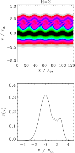
Figure 2: Simulations of the Wigner-Poisson and Vlasov-Poisson systems, at time $\omega_{p}t=200$, for $H=0$ (Vlasov, left frame), $H=1$ (middle frame), and $H=2$ (right frame). Initially monochromatic spectrum. Top panels: electron distribution function $f(x,v)$ in phase space. Bottom panels: spatially averaged electron distribution function $F(v)$ in velocity space.

To study the differences in the nonlinear evolution of the Wigner and Vlasov equations, we have simulated the well-known bump-on-tail instability, whereby a high-velocity beam is used to destabilize a Maxwellian equilibrium. We use the initial condition $f=(1+\delta)(n_{0}/\sqrt{2\pi}v_{th})[0.8\exp(-v^{2}/2v_{th}^{2})+0.4\exp(-2(v-2.5v_{th})^{2}/v_{th}^{2})]$, where $\delta$ represents random fluctuations of order $10^{-5}$ that help seed the instability (see Fig. 1). Here $v_{th}=\sqrt{k_{B}T_{e}/m}$ is the electron thermal speed. We use periodic boundary conditions with spatial period $L=40\pi\lambda_{De}$, where $\lambda_{De}=v_{th}/\omega_{p}$ is the Debye length. Three simulations were performed, with different values of the normalized Planck constant, defined as $H=\hbar\omega_{p}/mv_{th}^{2}$: $H=0$ (Vlasov), $H=1$, and $H=2$.

In order to highlight the transient oscillations in velocity space, we first perturb the above equilibrium with a monochromatic wave having $\lambda_{De}k=0.25$ (i.e., a wavelength of $8\pi\lambda_{De}$). Figures 2 shows the results from simulations of the Wigner-Poisson and Vlasov-Poisson systems. In both simulations, due to the bump-on-tail instability, electrostatic waves develop nonlinearly and create periodic trapped-particle islands (electron holes) with the wavenumber $k=0.25$. The theory described in the previous sections predicts the formation of velocity-space oscillations in the Wigner evolution, which should be absent in the classical (Vlasov) simulations. This is the case in the results presented in Fig. 2, where the oscillations are clearly visible.

In order to estimate their wavelength, a zoom on the spatially averaged electron distribution function $F(v)$ is shown in Fig. 3. According to the quasilinear theory, the velocity wavelength should be equal to $\lambda_{v}=\hbar k/m$ for the fundamental mode with $n=1$ [see Eq. (29)]. In our units, this yields $\lambda_{v}/v_{th}=Hk\lambda_{De}$, which is equal to 0.25 for $H=1$ and to 0.5 for $H=2$. The wavelengths observed in the simulations are slightly smaller: $\lambda_{v}/v_{th}\simeq 0.17$ and 0.35 for $H=1$ and $H=2$, respectively. However: (i) the oscillations are absent in the Vlasov case, as expected, (ii) the order of magnitude of the wavelength is correct, and (iii) the wavelength is proportional to $H$, in accordance with the quasilinear theory. The slight discrepancy in the observed value of $\lambda_{v}$ may have at least two origins. First, spatial wavenumbers different from $0.25$ can be excited due to the nonlinear mode coupling. Second, other modes with $n>1$ [see Eq. (29)] can affect the velocity-space wavelength.

Figure 3: Zoom on the spatially averaged electron distribution function $F(v)$ in velocity space for the same cases as in Fig. 2.

When the initial excitation is broad-band (i.e., wavenumbers $0.05\leq k\leq 0.5$ are excited), the electron holes start merging together at later times due to the sideband instability Kruer69 ; Albrecht07 (see Fig. 4). At this stage, mode coupling becomes important and quasilinear theory is not capable of describing these effects. As the system evolves toward larger spatial wavelength, the evolution becomes progressively more classical, with the appearance of a plateau in the resonant region. Nevertheless, at $\omega_{p}t=500$ the Wigner solution still displays some oscillatory behavior in velocity space, which is absent in the Vlasov evolution.

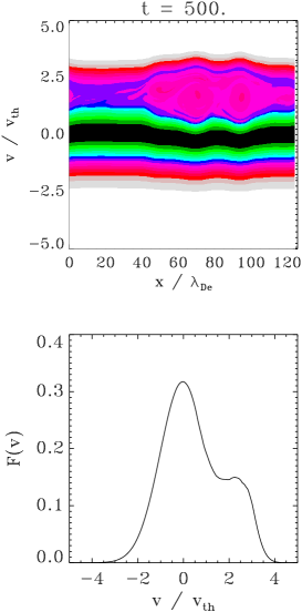
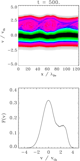
Figure 4: Simulations of the Wigner-Poisson and Vlasov-Poisson systems, for $\omega_{p}t=500$, for $H=0$ (Vlasov, left panel) and $H=1$ (Wigner, right panel). Initially broad wavenumber spectrum. Top panels: electron distribution function $f(x,v)$ in phase space. Bottom panels: spatially averaged electron distribution function $F(v)$ in velocity space.

Another set of simulations were performed for the case of a two-stream instability. The initial distribution function is composed of two Maxwellians with thermal speed $v_{th}$, each centered at $v=\pm 2v_{th}$ (see Fig. 5). Only the fundamental mode of the system, with the wavenumber $K=0.2\lambda_{De}^{-1}$, is excited, and it grows exponentially due to instability. Three simulations were performed, with different values of the normalized Planck constant: $H=0$ (Vlasov), $H=1$, and $H=2$. The expected oscillation wavelength in velocity space is $\lambda_{v}=\hbar K/m$. For the three simulated cases, it should take the values $\lambda_{v}=0$, $\lambda_{v}=0.2v_{th}$, and $\lambda_{v}=0.4v_{th}$. A zoom of the averaged Wigner function $F(v,t)$ around the velocity $v=0$ is plotted in Fig. 6 for the three cases, at time $\omega_{p}t=110$. The velocity-space oscillations are absent from the Vlasov simulation. In the Wigner cases, their wavelength is rather close to the theoretical value; in particular, it appears to grow with the scaled Planck constant, as expected from the theory. As in the bump-on-tail case, the oscillations tend to disappear over longer times.

Figure 5: Initial velocity distribution used in the simulations of the two-stream instability, both for the Vlasov and Wigner cases.

Figure 6: Zoom of the averaged Wigner distribution $F(v)$ for the two-stream instability at time $\omega_{p}t=110$. Top frame: $H=0$ (Vlasov); middle panel: $H=1$; bottom panel: $H=2$.

VI Conclusion

In this paper, the quasilinear theory for the Wigner-Poisson system was revisited. Conservation laws and the asymptotic solution were established. Distinctive quantum effects appear in the form of a transient oscillatory behavior in velocity space. Such quantum effects are favored when the energy spectrum is restricted to few modes. For longer times, the plasma tends to become classical – due to the spatial harmonic generation and the mode couplings – at least as far as the averaged Wigner function $F(v,t)$ is concerned. Thus, just as in the classical case, $F(v,t)$ evolves asymptotically toward a plateau in the resonant region of velocity space. It would be interesting to investigate whether monochromaticity enhances quantum effects in plasmas in general, which would represent a useful property for an experimental validation of the quantum plasma models.

Acknowledgments

This work was partially supported by the Alexander von Humboldt Foundation and by the Swedish Research Council.

References

- (1) F. Haas, G. Manfredi, and M. R. Feix, Phys. Rev. E 62, 2763 (2000).
- (2) G. Manfredi and F. Haas, Phys. Rev. B 64, 075316 (2001).
- (3) M. Marklund and G. Brodin, Phys. Rev. Lett. 98, 025001 (2007).
- (4) P. K. Shukla and B. Eliasson, Phys. Rev. Lett. 96, 245001 (2006); S. A. Khan and W. Masood, Phys. Plasmas 15, 062301 (2008).
- (5) Q. Haque and H. Saleem, Phys. Plasmas 15, 064504 (2008).
- (6) F. Haas and M. Lazar, Phys. Rev. E 77, 046404 (2008).
- (7) F. Haas, Phys. Plasmas 15, 022104 (2008).
- (8) L. N Tsintsadze and P. K. Shukla, J. Plasma Phys. 74, 431 (2008).
- (9) F. Haas, P. K. Shukla, and B. Eliasson, Nonlinear saturation of the Weibel instability in a dense Fermi plasma, J. Plasma Phys. 74, in press, 2008; doi: doi: 10.1017/S0022377808007368.
- (10) A. Bret, Phys. Plasmas 14, 084503 (2007).
- (11) V. Bychkov, M. Modestov, and M. Marklund, Phys. Plasmas 15, 032309 (2008).
- (12) P. K. Shukla and B. Eliasson, Phys. Rev. Lett. 100, 036801 (2008).
- (13) L. Wei and Y. N. Wang, Phys. Rev. B 75, 193407 (2007).
- (14) G. Manfredi and P.-A. Hervieux, Appl. Phys. Lett. 91, 061108 (2007).
- (15) G. Manfredi and P.-A. Hervieux, Phys. Rev. Lett. 97, 190404 (2006).
- (16) S. Ali, W. M. Moslem, I. Kourakis, and P. K. Shukla, New J. Phys. 10, 023007 (2008).
- (17) P. K. Shukla and L. Stenflo, Phys. Plasmas 13, 044505 (2006).
- (18) G. Brodin, M. Marklund, and G. Manfredi, Phys. Rev. Lett. 100, 175001 (2008).
- (19) M. Marklund, B. Eliasson, and P. K. Shukla, Phys. Rev. E 76, 067401 (2007); P. K. Shukla, Phys. Lett. A 369, 312 (2007).
- (20) D. Shaikh and P. K. Shukla, Phys. Rev. Lett. 99, 125002 (2007); New J. Phys. 10, 083007 (2008).
- (21) A. A. Vedenov, E. P. Velikhov, and R. Z. Sagdeev, Nucl. Fusion 1, 82 (1961).
- (22) Yu. A. Romanov and G. F. Filippov, Sov. Phys. JETP 13, 87 (1961).
- (23) A. A. Vedenov, E. P. Velikhov, and R. Z. Sagdeev, Nucl. Fusion Suppl. 2, 465 (1962).
- (24) W. E. Drummond and D. Pines, Nucl. Fusion Suppl. 3, 1049 (1962).
- (25) D. Pines and J. R. Schrieffer, Phys. Rev. 125, 804 (1962).
- (26) N. Matsudaira, Phys. Fluids 9, 539 (1966).
- (27) V. Arunasalam, Phys. Rev. 149, 102 (1966).
- (28) V. Arunasalam, Phys. Rev. A 7, 1353 (1973).
- (29) B. N. Breizman and J. Weiland, Eur. J. Phys. 7, 222 (1986).
- (30) A. A. Vedenov, Dokl. Akad. Nauk SSSR 147, 334 (1962).
- (31) G. Laval and D. Pesme, Plasma Phys. Control. Fusion 41, A239 (1999).
- (32) Yu. L. Klimontovich and V. P. Silin, in Plasma Physics, ed. J. Drummond (McGraw-Hill, New York, 1961).
- (33) G. Manfredi and M. R. Feix, Phys. Rev. E 62, 4665 (2000).
- (34) F. Haas, G. Manfredi, and J. Goedert, Phys. Rev. E 64, 026413 (2001).
- (35) N. Suh, M. R. Feix, and P. Bertrand, J. Comput. Phys. 94, 403 (1991).
- (36) W. L. Kruer, J. M. Dawson, R. N. Sudan, Phys. Rev. Lett. 23, 838 (1969).
- (37) M. Albrecht-Marc, A. Ghizzo, T. W. Johnston, T. Réveillé, D. Del Sarto, and P. Bertrand, Phys. Plasmas 14, 072704 (2007).