Turbulent magnetic Prandtl numbers obtained with MHD Taylor-Couette flow experiments

Abstract

The stability problem of MHD Taylor-Couette flows with toroidal magnetic fields is considered in dependence on the magnetic Prandtl number. Only the most uniform (but not current-free) field with $B_{\rm in}=B_{\rm out}$ has been considered. For high enough Hartmann numbers the toroidal field is always unstable. Rigid rotation, however, stabilizes the magnetic (kink-)instability.

The axial current which drives the instability is reduced by the electromotive force induced by the instability itself. Numerical simulations are presented to probe this effect as a possibility to measure the turbulent conductivity in a laboratory. It is shown numerically that in a sodium experiment (without rotation) an eddy diffusivity 4 times the molecular diffusivity appears resulting in a potential difference of $\sim 34$ mV/m. If the cylinders are rotating then also the eddy viscosity can be measured. Nonlinear simulations of the instability lead to a turbulent magnetic Prandtl number of 2.1 for a molecular magnetic Prandtl number of $0.01$. The trend goes to higher values for smaller Pm.

I Introduction

Strong enough toroidal fields that are not current-free become unstable due to the Tayler instability (TI, T57 ; V72 ; T73 ). Because the source of the energy is the electric current, these (mainly nonaxisymmetric) instabilities can exist even without any rotation. On the other hand, it is becoming increasingly clear that the stability of differential rotation under the presence of magnetic fields is one of the key problems in MHD astrophysics. There, however, is no laboratory experiment so far and even the related numerical simulations of TI are very rare BRW06 ; GRE08 . We shall demonstrate here how the TI interacts with differential rotation, and how it is possible to verify the main results in laboratory experiments. In particular, the theoretical results are used to propose experiments for measuring the turbulent diffusivity via a TI-induced reduction of the electromotive force. Such experiments will be of high relevance as the knowledge of the magnetic turbulent diffusivity is basic for many applications in fluid dynamics. Very often we have only limited informations about the magnetic diffusivity. In the laboratory only a very small number of experiments have been done (see RB01 ; Frick07 ). The same is true for the eddy viscosity which can be measured with the same experimental device so that finally the turbulent magnetic Prandtl number becomes known for one and the same instability.

Consider a Taylor-Couette (TC) flow with $U$ as the velocity, $B$ the magnetic field, $\nu$ the microscopic kinematic viscosity and $\eta$ the microscopic magnetic diffusivity. The basic state in cylindrical geometry is $U_{R}=U_{z}=B_{R}=B_{z}=0$ and

$$U_{\phi}=R\Omega=a_{\Omega}R+\frac{b_{\Omega}}{R},\qquad B_{\phi}=a_{B}R+\frac{b_{B}}{R}.$$ (1)

Let

$$\hat{\eta}=\frac{R_{\rm{in}}}{R_{\rm{out}}},\;\;\;\mu_{\Omega}=\frac{\Omega_{\rm{out}}}{\Omega_{\rm{in}}},\;\;\;\mu_{B}=\frac{B_{\rm{out}}}{B_{\rm{in}}}.$$ (2)

$R_{\rm{in}}$ and $R_{\rm{out}}$ are the radii of the inner and outer cylinders, $\Omega_{\rm{in}}$ and $\Omega_{\rm{out}}$ their rotation rates and $B_{\rm{in}}$ and $B_{\rm{out}}$ are the azimuthal magnetic fields at the inner and outer cylinders. In particular, a field of the form $b_{B}/R$ is generated by an axial current only through the inner region $R<R_{\rm{in}}$, whereas a field of the form $a_{B}R$ is generated by a uniform axial current through the entire region $R<R_{\rm{out}}$ including the fluid.

The magnetic Prandtl number $\mathrm{Pm}$, the Reynolds number $\mathrm{Re}$ and the Hartmann number $\mathrm{Ha}$,

$${\rm Pm}=\frac{\nu}{\eta},\quad{\rm{Re}}=\frac{\Omega_{\rm{in}}R_{0}^{2}}{\nu},\quad{\rm{Ha}}=\frac{B_{\rm{in}}R_{0}}{\sqrt{\mu_{0}\rho\nu\eta}},$$ (3)

are the basic parameters of the problem where $R_{0}=\sqrt{DR_{\rm in}}$ is the unit of length with $D=R_{\rm{out}}-R_{\rm{in}}$. For the velocity the boundary conditions are assumed as always no-slip ($\mbox{\boldmath$u$}=0$). For conducting walls the radial component of the field and the tangential components of the current must vanish so that ${\rm d}b_{\phi}/{\rm d}R+b_{\phi}/R=b_{R}=0$ at both $R_{\rm{in}}$ and $R_{\rm{out}}$. Here $u$ and $b$ are the fluctuating components of flow and field.

While the linear stability code works well with small $\mathrm{Pm}$, the minimum microscopic $\mathrm{Pm}$ which can be handled with our nonlinear code is (only) $10^{-2}$. The numerics cannot deal with the very small magnetic Prandtl numbers of liquid metals used in the laboratory ($\rm Pm\lower 1.72218pt\hbox{$\;\buildrel<\over{\scriptstyle\sim}\;$}10^{-5}$). Some of our results can only be obtained by extrapolation methods.

II The instability map

The map for the marginal instability is the result of a linear theory for liquid sodium with $\mathrm{Pm}=10^{-5}$. The linearized equations of the MHD system in a TC flow under the presence of a toroidal field are given elsewhere, RHSE07 .

Figure 1 shows the results for various values of $\mu_{B}$. For $\mu_{B}=0.5$ the toroidal field is current-free between the cylinders. The outer cylinder is assumed as resting so that for vanishing magnetic field the rotation law is centrifugally-unstable for $\rm Re>68$. From the given profiles closest to being current-free is $\mu_{B}=0$ and we do not find that for $\mathrm{Ha}\leq 200$ there is any sign of destabilizing influence of the magnetic field, for neither axisymmetric nor nonaxisymmetric perturbations.

For certain $\mu_{B}$ the $m=1$ mode should be unstable while the $m=0$ mode should be stable S06 . The values $\mu_{B}=1$ and $\mu_{B}=2$ in Fig. 1 are examples of this situation. There is always a crossover point at which the most unstable mode changes from $m=0$ to $m=1$. Note also that for $\mu_{B}=1$ the critical Reynolds number for the $m=0$ mode steadily increases, while the $m=1$ mode is suddenly decreasing for a sufficiently strong magnetic field. Hence, weak fields initially can stabilize the flow, and stronger fields eventually destabilize via a nonaxisymmetric mode. Beyond $\mathrm{Ha}=150$ the flow is unstable even for $\mathrm{Re}=0$.

Except for the almost current-free profile $\mu_{B}=0$ all other values share the feature that there is a critical Hartmann number beyond which the basic state is unstable even for $\mathrm{Re}=0$. Let Ha⁽⁰⁾ and Ha⁽¹⁾ denote these critical Hartmann numbers for $m=0$ and $m=1$, resp.

Figure 1: The marginal stability curves for $m=0$ (dashed) and $m=1$ (solid). Pm$=10^{-5}$, $\hat{\eta}=0.5$, $\mu_{\Omega}=0$, and $\mu_{B}$ as indicated. Conducting walls. The hatched domain is stable.

II.1 Flat rotation laws

The rotation law with resting outer cylinder destabilizes the magnetic field. The question arises what happens for those flat rotation laws which are stable in the nonmagnetic regime. In Fig. 2 the marginal stability curves are also given for ${\mu}_{\Omega}=0.25$ (Rayleigh limit), ${\mu}_{\Omega}=0.35$, ${\mu}_{\Omega}=0.45$ and ${\mu}_{\Omega}=1$ (rigid rotation). One finds the instabilities more and more stabilized by the rotation.

Note the massive quenching of the TI by rigid rotation. Even a rather slow rotation prevents the TI to destabilize the system. Rigidly rotating containers can keep much stronger fields as stable than without rotation. This rotational stabilization is modified for nonuniform rotation. At the Rayleigh limit, where $\Omega\propto R^{-2}$, even a slow rotation destabilizes the system while it is stabilized for fast rotation. Generally, fast rotation stabilizes, slow rotation destabilizes. At a Hartmann number of (say) 50 and at the Rayleigh line one finds for increasing rotation rate the regimes: stable, unstable, stable. The critical Reynolds numbers of the sequence are $\sim 300$ and $\sim 1800$ which can easily be realized in the laboratory. A similar situation holds for the (quasi-Kepler) rotation law with ${\mu}_{\Omega}=0.35$ while for rotation laws with ${\mu}_{\Omega}\lower 1.72218pt\hbox{$\;\buildrel>\over{\scriptstyle\sim}\;$}0.45$ only the rotational stabilization can be observed.

Figure 2: $\mu_{B}=1$. The same magnetic constellation as in Fig. 1 (middle) but for ${\mu}_{\Omega}$ as indicated. ${\mu}_{\Omega}=0$ (resting outer cylinder), ${\mu}_{\Omega}=0.25$ (Rayleigh limit), ${\mu}_{\Omega}=0.35$, ${\mu}_{\Omega}=0.45$, ${\mu}_{\Omega}=1$ (rigid rotation). The dotted line gives the eigenvalues for $m=0$ which for those parameters only exists for ${\mu}_{\Omega}=0$.

II.2 Electric currents

For experiments the electric currents must not be too strong. As an upper limit currents with 10–15 kA shall be considered. In order to translate the obtained critical Hartman numbers into amplitudes of electrical currents we apply our results to liquid sodium with a density of 0.92 g/cm³, a microscopic magnetic diffusivity of 810 cm²/s and a magnetic Prandtl number of $10^{-5}$. For gallium-indium-tin the necessary currents are stronger by a factor of 3.15 (see RSSH07 ).

Let $I_{\rm{axis}}$ be the axial current inside the inner cylinder and $I_{\rm{fluid}}$ the axial current through the fluid (i.e. between inner and outer cylinder). Then the toroidal field amplitudes at the inner and outer cylinders are

$$B_{\rm{in}}=\frac{I_{\rm{axis}}}{5R_{\rm{in}}},\qquad B_{\rm{out}}=\frac{(I_{\rm{axis}}+I_{\rm{fluid}})}{5R_{\rm{out}}},$$ (4)

measured in cm, Gauss and Ampere. Expressing $I_{\rm{axis}}$ and $I_{\rm{fluid}}$ in terms of our dimensionless parameters one finds

$$I_{\rm{axis}}=5{\rm Ha}\ \sqrt{\frac{\hat{\eta}\mu_{0}\rho\nu\eta}{1-\hat{\eta}}},\quad\quad I_{\rm{fluid}}=\frac{\mu_{B}-\hat{\eta}}{\hat{\eta}}I_{\rm{axis}}.$$ (5)

Table 1 gives the electric currents needed to reach the less of Ha⁽⁰⁾ and Ha⁽¹⁾ for $\hat{\eta}=0.5$, and $\mu_{B}$ ranging from $-2$ to 2 in each case. Note that for large $|\mu_{B}|$ the current $I_{\rm{fluid}}$ approaches a constant value.

Table 1: Characteristic Hartmann numbers and electric currents for a sodium-container ($\hat{\eta}=0.5$) with conducting walls. The experiment with the almost uniform field $\mu_{B}=1$ is indicated in bold.

$\mu_{B}$	$\mathrm{Ha}^{(0)}$	$\mathrm{Ha}^{(1)}$	$I_{\rm{axis}}$ [kA]	$I_{\rm{fluid}}$ [kA]
-2	19.8	24.8	0.807	-4.04
-1	59.3	63.7	2.42	-7.25
1	$\infty$	151	6.16	6.16
2	$\infty$	35.3	1.44	4.32

The most interesting experiment is that with the almost uniform field $\mu_{B}=1$. For a container with a gap of $\hat{\eta}=0.5$, parallel currents of 6.16 kA are necessary along the axis and through the fluid. The experiment does not possess the weakest electric currents but both the currents are parallel and have the same amplitudes. Figure 1 (middle) shows that in this case a crossing point M exists where the axisymmetric mode has the same characteristic Reynolds number and Hartmann number as the nonaxisymmetric mode with $m=1$.

III The eddy diffusivity

We now turn to the mean-field concept turbulent fluids of electrically conducting material. It is known that the existence of turbulence in the fluid reduces the electric conductivity or – with other words – the fluctuations enhance the magnetic diffusivity called the turbulent magnetic diffusivity. In MHD the turbulent diffusivity is a much more simple quantity than the corresponding eddy viscosity. While the latter is also formed by the existing magnetic fluctuations this is not the case for the turbulent diffusivity. In a simplified (‘SOCA’) approximation for a turbulence field with a correlation time $\tau_{\rm corr}$ results

$$\nu_{T}\simeq(\frac{2}{15}\langle u^{2}\rangle+\frac{1}{3}\frac{\langle b^{2}\rangle}{\mu_{0}\rho})\ \tau_{\rm corr}$$ (6)

for the eddy viscosity but only

$$\eta_{T}\simeq\frac{\tau_{\rm corr}}{3}\langle u^{2}\rangle$$ (7)

for the eddy diffusivity, VK83 . The magnetic fluctuations do not contribute to the magnetic diffusivity. This basic difference between both the diffusion coefficients is not yet proven by an experiment. The results (6) and (7) suggest that in turbulent magnetic fluids the effective magnetic Prandtl number exceeds the value 0.4 which was confirmed by numerical simulations for driven MHD turbulence with Pm of order unity, YOUS03 . The knowledge of the turbulent magnetic Prandtl number is of extraordinary meaning in fluid mechanics and geo/astrophysics. For its calculation one has to measure both quantities simultaneously in one and the same experiment.

Simplifying, the nonaxisymmetric components of flow and field may be used in the following as the ‘fluctuations’ while the axisymmetric components are considered as the mean quantities. Then the averaging procedure is simply the integration over the azimuth $\phi$. It is standard to express the turbulence-induced electromotive force (EMF) as

$$\mbox{\boldmath$\cal{E}$}=\langle\mbox{\boldmath$u$}\times\mbox{\boldmath$b$}\rangle=-\eta_{\rm T}{\rm curl}\mbox{\boldmath$B$}$$ (8)

with the (scalar) eddy diffusivity $\eta_{\rm T}$ which must be positive. In cylindric geometry the mean current ${\rm curl}\mbox{\boldmath$B$}$ has only a $z$-component. Hence,

$${\cal E}_{z}=-\eta_{\rm T}{\rm curl}_{z}\mbox{\boldmath$B$}.$$

Take from Table 1 that for $\mu_{B}=1$ the current through the fluid is positive then for negative ${\cal E}_{z}$ the $\eta_{\rm T}$ results as positive. This is indeed the case. We have shown that TI indeed provides reasonable expressions for the turbulent diffusivity in rotating containers, RGS08 .

III.1 Nonlinear simulations

The absolute values for ${\cal E}_{z}$ can only be computed with nonlinear simulations. The minimum possible magnetic Prandtl number for the code yielding robust results is $10^{-2}$. Here the results without and with rotation but only for $\mathrm{Ha}=200$ are reported. The used MHD Fourier spectral element code has been described earlier in more detail, FOURN05 , GRF07 .

Either $M=8$ or $M=16$ Fourier modes are used, two or three elements in radius and twelve or eighteen elements in axial direction, resp. The polynomial order is varied between $N=8$ and $N=16$.

Figure 3 shows the negative TI-induced EMF for magnetic Prandtl numbers varied between 0.01 to 1. The main results are that i) the EMF is always negative ($\eta_{\rm T}$ positive!) and ii) it runs with $E/\mathrm{Pm}$ with the factor $E\simeq 3$ taken from the plot. The resulting EMF in physical units is $-\eta EB_{0}/D$. Hence,

$$\frac{\eta_{\rm T}}{\eta}\simeq 1.5E\simeq 4.5.$$ (9)

For the voltage difference $\delta U$ due to this EMF one finds $\delta U=\eta EB_{0}H/D$ with $H$ as the container height and

$$\delta U=\frac{\eta E\Gamma\sqrt{\mu_{0}\rho\nu\eta}{\rm Ha}}{D}$$ (10)

with $\Gamma=H/D$ the aspect ratio of the container. For $D=10$ cm and $H=100$ cm we find for sodium ($\sqrt{\mu_{0}\rho\nu\eta}\simeq 8.15$) the maximum value of 34 mV as the potential difference from endplate to endplate. This value can only be considered as an estimate basing on the scaling with $1/\mathrm{Pm}$ suggested by Fig. 3. But even in the case that the slope of the curve decreases for smaller $\mathrm{Pm}$ the effect should be observable in the laboratory. A Hartmann number of 200 requires 163 G at the inner cylinder ($R_{\rm in}=10$ cm) which can be produced with an axial current of 8.15 kA for $R_{\rm out}=2R_{\rm in}$.

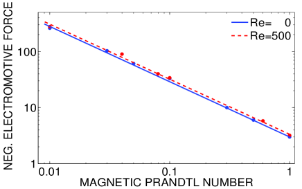
Figure 3: Maximum values of the normalized axial EMF vs $\mathrm{Pm}$ for $\mathrm{Ha}=200$ and $\mu_{B}=1$. The lower curve is without rotation, the upper curve is with rotation and shear ($\mathrm{Re}=500,{\mu}_{\Omega}=0.35$).

In order to study the rotational influence also the Pm-dependence of the EMF under the presence of a differential rotation is given in Fig. 3. It is ${\mu}_{\Omega}=0.35$ (quasikeplerian) and the Reynolds number is $\mathrm{Re}=500$. Note that the influence of the rotation for the TI-induced EMF is surprisingly weak; with rotation the values are slightly higher than without rotation.

The magnetic Reynolds number, $\mathrm{Rm}={\rm MAX}(u)D/\eta$, of the fluctuations is considered next. With Fig. 4 a rather weak magnetic Prandtl number dependence of $\mathrm{Rm}$ is found. Extrapolating the results to $\rm Pm=10^{-5}$ gives in both cases a value of $\mathrm{Rm}\simeq 2.6$. The associated velocity fluctuations for sodium are about 15 m/s in a gap of 1 cm and 1.5 m/s in a gap of 10 cm. The values are rather similar to those of the Riga ’$\alpha$-yashchik’ experiment, KR80 . Even with resting cylinders it is possible to produce rather high (azimuthal) velocities in TI experiments.

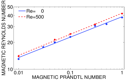
Figure 4: The same as in Fig. 3 but for the magnetic Reynolds number of the fluctuations.

IV The eddy viscosity

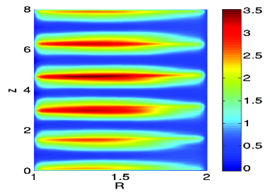
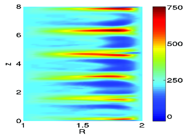
Figure 5: $\mathrm{Ha}=200$, $\mathrm{Re}=500$. Simulations for a flow with $\mathrm{Pm}=0.01$, ${\mu}_{\Omega}=0.35$ and $\mu_{B}=1$. Left: $\eta_{\rm T}/\eta$, right: $\nu_{\rm T}/\nu$. The resulting magnetic Prandtl number $\nu_{\rm T}/\eta_{\rm T}$ is about 2.1.

Experiments with Tayler instability under the presence of differential rotation can also provide eddy viscosity measurements due to the angular momentum transport by both Reynolds stress and Maxwell stress. Within the diffusion approximation it is

$$T=\langle u_{R}^{\prime}u_{\phi}^{\prime}\rangle-\frac{\langle B_{R}^{\prime}B_{\phi}^{\prime}\rangle}{\mu_{0}\rho}=-\nu_{\rm T}R\frac{{\rm d}\Omega}{{\rm d}R}$$ (11)

for the torque in the fluid. The fluctuations of flow and field can be calculated with the code. The patterns for the instability-induced diffusivity values for $\rm Pm=0.01$ are shown in Fig. 5 for the same model as used in Fig 3, i.e. ${\mu}_{\Omega}=0.35$, $\mathrm{Ha}=200$ and $\mathrm{Re}=500$. One finds the turbulence-originated increase of the eddy viscosity $\nu_{\rm T}/\nu$ much larger than for the turbulent diffusivity. The turbulent magnetic Prandtl number $\rm Pm_{\rm T}=\nu_{\rm T}/\eta_{\rm T}$ becomes about 2.05. Similar calculations for $\mathrm{Pm}=0.1$ lead to $\rm Pm_{\rm T}=0.71$ while for $\mathrm{Pm}=1$ the smaller value 0.65 results. The results only weakly depend on the averaging procedure. The given numbers follow after averaging over the whole cylinder. The turbulent magnetic Prandtl number slightly increases with decreasing microscopic $\mathrm{Pm}$; and for small Pm it reaches values larger than unity. Note the differing results of simulations with Pm much smaller than unity and those with $\rm Pm\lower 1.72218pt\hbox{$\;\buildrel<\over{\scriptstyle\sim}\;$}1$, YOUS03 .

Small $\mathrm{Pm}$ are shown to produce large turbulent values $\rm Pm_{\rm T}$. We cannot provide results for $\mathrm{Pm}$ smaller than $0.01$ so far. Only laboratory experiments utilizing Tayler instability in liquid metals with their very small magnetic Prandtl number are able to show whether the obtained trend is a general one.

References

- (1) R. J. Tayler, Proc. Phys. Soc. B 70, 31 (1957)
- (2) Y. V. Vandakurov, SvA 16, 265 (1972).
- (3) R. J. Tayler, MNRAS 161, 365 (1973).
- (4) J. Braithwaite, Astron. Astrophys. 449, 451 (2006).
- (5) M. Gellert, G. Rüdiger, and D. Elstner, Astron. Astrophys. 479, L33 (2008).
- (6) A. B. Reighard and M. R. Brown, Phys. Rev. Lett. 86, 2794 (2001).
- (7) P. Frick, S. Denisov, V. Noskov, and R. Stepanov, Astron. Nachr. 329, 706 (2008).
- (8) G. Rüdiger et al., MNRAS 377, 1481 (2007).
- (9) D. Shalybkov, Phys. Rev. E 73, 16302 (2006).
- (10) G. Rüdiger, M. Schultz, D. Shalybkov, and R. Hollerbach, Phys. Rev. E 76, 056309 (2007).
- (11) S. I. Vainshtein, and L. L. Kichatinov, Geophys. Astrophys. Fluid Dyn. 24, 273 (1983).
- (12) T. A. Yousef, A. Brandenburg, and G. Rüdiger, Astron. Astrophys. 411, 321 (2003).
- (13) G. Rüdiger, M. Gellert, and M. Schultz, MNRAS submitted.
- (14) A. Fournier et al., J. Comput. Phys. 204, 462 (2005).
- (15) M. Gellert, G. Rüdiger, and A. Fournier, Astron. Nachr. 328, 1162 (2007).
- (16) F. Krause and K-H. Rädler, Mean-field magnetohydrodynamics and dynamo theory (Akademieverlag Berlin, 1980) .