Fermi-Surface Reconstruction in the Periodic Anderson Model

Abstract

We study ground state properties of periodic Anderson model in a two-dimensional square lattice with variational Monte Carlo method. It is shown that there are two different types of quantum phase transition: a conventional antiferromagnetic transition and a Fermi-surface reconstruction which accompanies a change of topology of the Fermi surface. The former is induced by a simple back-folding of the Fermi surface while the latter is induced by localization of $f$ electrons. The mechanism of these transitions and the relation to the recent experiments on Fermi surface are discussed in detail.

1 Introduction

Recently, antiferromagnetic (AF) transition which accompanies an abrupt change of Fermi surface has been widely observed in heavy fermion compounds and has attracted much attention. De Haas-van Alphen (dHvA) experiments in Ce compounds, such as CeRh₂Si₂ [1], CeIn₃ [2] and CeRhIn₅ [3], show that the topology of Fermi surface abruptly changes across the AF transition under pressure. According to band calculations, Fermi surface in the AF phase is well explained by a 4$f$-localized model while that in the paramagnetic phase is well explained by a 4$f$-itinerant model [1, 2, 3, 4]. This Fermi-surface change has also been suggested in the Hall effect experiment in YbRh₂Si₂ [5]. Although the Hall coefficient shows a continuous change as a function of magnetic field at finite temperature, its slope becomes sharper with decreasing temperature. From this, it is claimed that there will be a discontinuous jump of the Hall coefficient at the AF quantum critical point (QCP) at $T=0$. This means that a change from a “small Fermi surface” (AF side) to a “large Fermi surface” (paramagnetic side) occurs at QCP. In these experiments, the AF transition and the abrupt change of the Fermi surface seem to occur simultaneously. On the other hand, in CeRh_1-xCo_xIn₅, an abrupt change of the Fermi surface is observed at $x=0.3\sim 0.4$ while the AF QCP exists at $x=0.7\sim 0.8$ [6, 7]. In this case, the AF transition and the abrupt change of the Fermi surface are not necessarily coincident and the relation between them has not been clarified yet.

In a conventional picture of the QCP in heavy fermion system, the AF transition is induced by the competition between Kondo screening and RKKY interaction [8]. In this case, the conduction electrons ($c$ electrons) and the localized $f$ electrons hybridize with each other and form the composite quasiparticles. The $f$ electrons obtain the itinerancy through the hybridization and the AF transition is expected to be described by a so-called Moriya-Hertz-Millis (MHM) theory [9, 10, 11]. This picture have been extensively studied so far and succeeded in describing the unconventional phenomena such as a non-Fermi-liquid behavior around the QCP. However, it is not clear whether the MHM theory can be applied or not to the case where the $f$ electrons are strongly localized and the itinerant picture becomes inappropriate. Indeed, the change of the topology of the Fermi surface mentioned above cannot be explained by the simple back-folding of the Fermi surface which is based on the itinerant picture.

Recently, on the other hand, novel type of theory which considers the localization of $f$ electrons has been proposed by some authors [12, 13, 14, 15, 16]. It is based on the breakdown of the Kondo screening or the decoupling of $c$ and $f$ electrons. In this case, the change of nature of the $f$ electrons at the QCP has been emphasized, but the details are still uncertain.

With these facts in mind, we studied the ground state phase diagram of the Kondo lattice model (KLM) in the previous work [17]. This model is one of the simplest models which contain $c$ and $f$ electrons and describe the heavy-fermion system. We have found that there are two types of quantum phase transitions: a conventional AF transition and a topological transition of a Fermi surface (Fermi-surface reconstruction). The former transition is induced by the folding of the Fermi surface and therefore we denote as “conventional”. In the latter transition, on the other hand, the Kondo screening becomes almost irrelevant (but does not disappear) and almost fully polarized AF state appears accompanied with the change of the topology of the Fermi surface.

In this paper, we study the ground state properties of the periodic Anderson model (PAM). The KLM will not be enough to discuss the issue of the itinerancy and localization of $f$ electrons, since the $f$ electrons are always localized in the KLM. On the other hand, in the PAM, we can control the number of $f$ electrons and can discuss the change of the nature of $f$ electrons by changing the parameters such as $U$ (on-site Coulomb interaction), $V$ ($c$-$f$ hybridization) and $E_{f}$ (energy level of $f$ electrons). Moreover, we discuss the properties of the Fermi surface in detail by calculating the momentum distribution function which was not discussed in the previous paper on the KLM [17]. We show that the Fermi-surface reconstruction observed in the KLM also occurs in the PAM under the condition of $U=\infty$ and sufficiently low values of $E_{f}$. The Fermi-surface reconstruction have two remarkable aspects as a quantum phase transition. It can be regarded as a kind of Lifshitz transition, where the topology of the Fermi surface changes from hole-like to electron-like. At the same time, it can be regarded as a kind of Mott transition, where the $f$ electrons change their character from itinerant to localized.

The organization of this paper is as follows. In §2, we introduce the model and variational wave functions. In §3, we show the results of VMC calculation. The ground state phase diagrams and some physical quantities are studied in detail. In §4, we discuss the relation between our results and the experiments. §5 is devoted to the summary.

2 Model and Method

We study the following PAM in a two-dimensional square lattice,

$$H=\sum_{\bm{k}\sigma}\varepsilon_{\bm{k}}c_{\bm{k}\sigma}^{\dagger}c_{\bm{k}\sigma}+E_{f}\sum_{i\sigma}n^{f}_{i\sigma}\\ -V\sum_{i\sigma}(f^{\dagger}_{i\sigma}c_{i\sigma}+\mathrm{h.c.})+U\sum_{i}n^{f}_{i\uparrow}n^{f}_{i\downarrow},$$ (1)

where $\varepsilon_{\bm{k}}$, $E_{f}$, $V$ and $U$ represent energy dispersion of $c$ electrons, energy level of $f$ electrons, hybridization between $c$ and $f$ electrons and on-site Coulomb interaction between $f$ electrons, respectively. In the PAM, the number of $f$ electrons at each site is not fixed and therefore the total electron density $n=n_{c}+n_{f}$ is a controlling parameter.

The trial wave function for a paramagnetic state is expressed as,

$$\left|\Psi\right>=P^{f}_{\mathrm{G}}\left|\Phi\right>=P^{f}_{\mathrm{G}}\prod_{\bm{k}\sigma}(u_{\bm{k}}c^{\dagger}_{\bm{k}\sigma}+v_{\bm{k}}f^{\dagger}_{\bm{k}\sigma})\left|0\right>$$ (2)

with

$$P^{f}_{\mathrm{G}}=\prod\left(1-(1-g)n^{f}_{i\uparrow}n^{f}_{i\downarrow}\right),$$ (3)

and

$$u^{2}_{\bm{k}} =\frac{1}{2}\left[1-\frac{\varepsilon_{\bm{k}}-\tilde{E_{f}}}{\sqrt{(\varepsilon_{\bm{k}}-\tilde{E_{f}})^{2}+4\tilde{V}^{2}}}\right],$$ (4)

$$v^{2}_{\bm{k}} =\frac{1}{2}\left[1+\frac{\varepsilon_{\bm{k}}-\tilde{E_{f}}}{\sqrt{(\varepsilon_{\bm{k}}-\tilde{E_{f}})^{2}+4\tilde{V}^{2}}}\right].$$ (5)

Here $u_{\bm{k}}$ $(v_{\bm{k}})$ corresponds to the mixing amplitude of $c$ ($f$) electrons. $P^{f}_{\mathrm{G}}$ is a Gutzwiller projection operator which reduces the probability of double occupancy of $f$ electrons at the same site. Since we consider the case of $U=\infty$, we set $g=0$ in the following. The unprojected wave function $\left|\Phi\right>$ is obtained by diagonalizing the following one-body Hamiltonian,

$$H=\sum_{\bm{k}\sigma}\left(c_{\bm{k}\sigma}^{\dagger},f_{\bm{k}\sigma}^{\dagger}\right)\begin{pmatrix}\varepsilon_{\bm{k}}&-\tilde{V}\\ -\tilde{V}&\tilde{E_{f}}\end{pmatrix}\begin{pmatrix}c_{\bm{k}\sigma}\\ f_{\bm{k}\sigma}\end{pmatrix}.$$ (6)

It is just the $U=0$ PAM with “effective” hybridization $\tilde{V}$ and “effective” $f$-electron level $\tilde{E_{f}}$. $\tilde{V}$ and $\tilde{E_{f}}$ are variational parameters and they are optimized so as to minimize the variational energy. This form of trial wave function is also used in ref. Shiba1 for a one-dimensional case. As an AF trial wave function, we construct a state $\left|\Phi\right>$ by diagonalizing the following Hamiltonian,

$$H =\sum_{\bm{k}\sigma}\left(c_{\bm{k}\sigma}^{\dagger},c_{\bm{k}+\bm{Q}\sigma}^{\dagger},f_{\bm{k}\sigma}^{\dagger},f_{\bm{k}+\bm{Q}\sigma}^{\dagger}\right)\times$$

$$\begin{pmatrix}\varepsilon_{\bm{k}}&\sigma\Delta_{c}&-\tilde{V}&0\\ \sigma\Delta_{c}&\varepsilon_{\bm{k}+\bm{Q}}&0&-\tilde{V}\\ -\tilde{V}&0&\tilde{E_{f}}&-\sigma\Delta_{f}\\ 0&-\tilde{V}&-\sigma\Delta_{f}&\tilde{E_{f}}\end{pmatrix}\begin{pmatrix}c_{\bm{k}\sigma}\\ c_{\bm{k}+\bm{Q}\sigma}\\ f_{\bm{k}\sigma}\\ f_{\bm{k}+\bm{Q}\sigma}\end{pmatrix},$$ (7)

with $\bm{Q}=(\pi,\pi)$ being an AF ordering vector. Here $\Delta_{c}$ and $\Delta_{f}$ represent the variational parameters of AF gap in $c$ and $f$ electrons, respectively. The summation over $\bm{k}$ is carried out in the folded AF Brillouin zone. If we set $\Delta_{c}=\Delta_{f}=0$, eq. (7) reduces to eq. (6). Although the choice of the basis and the notation of variational parameters are slightly different from those used in ref. Watanabe, the obtained unprojected band dispersion is the same with the previous paper [17] ($\Delta_{f}$ and $\Delta_{c}$ corresponds to $M$ and $m$ in ref. Watanabe).

We optimize the four variational parameters $(\tilde{V},\tilde{E_{f}},\Delta_{f},\Delta_{c})$ and find the lowest energy state in a $V$-$n$ phase diagram. Possible candidates for the ground state are classified according to the shape of the Fermi surface and the band dispersion of the one-body part $\left|\Phi\right>$: paramagnetic metal (PM), AF metal with hole-like Fermi surface (AF_h), AF metal with electron-like Fermi surface (AF_e) and AF metal with $\tilde{V}=0$ (AF_S, S denotes “small”). This notation is the same with that in the previous paper [17] and the schematic Fermi surfaces are shown in Fig. 1. In PM, AF_h and AF_e, $\tilde{V}$ is finite and the one-body part forms the $c$-$f$ hybridized band. It is based on the concept of “large” Fermi surface. In contrast, $\tilde{V}=0$ in AF_S, and $c$ and $f$ electrons form their band dispersions individually. AF_S is based on the concept of “small” Fermi surface. However, note that the expressions of “large” and “small” Fermi surface are not appropriate in the AF state since the volumes of the Fermi surface are the same in AF_h, AF_e and AF_S. Moreover, AF_e and AF_S have the same Fermi-surface topology and cannot be distinguished from each other only by the Fermi surface. The difference between them are discussed in the next section.

3 Results

3.1 Ground State Phase Diagram

We show the ground state phase diagrams for different values of $E_{f}$ in Fig. 1. The system sizes are set to be 8$\times$8, 10$\times$10 and 12$\times$12 with periodic-antiperiodic boundary condition. When $E_{f}=0.0$, the state changes from PM to AF_h at $V=V_{\mathrm{AF}}$ as shown in Fig. 1(a). The first Brillouin zone is folded and the AF gap opens along the newly formed AF Brillouin zone boundary. This is a “conventional” second-order AF transition. The region of AF_h extends to $V\rightarrow 0$. On the other hand, when $E_{f}=-0.2$, a novel type of quantum phase transition occurs and AF_e is realized for $V<V_{\mathrm{FS}}$, as shown in Fig 1(b). At $V=V_{\mathrm{FS}}$, the band dispersion discontinuously changes from convex upward (AF_h side) to convex downward (AF_e side). It is regarded as a kind of Lifshitz transition, where the topology of the Fermi surface changes. We call this transition a “Fermi-surface reconstruction” and its origin is discussed in §3.2 in detail. As $E_{f}$ becomes lower, the region of AF_e becomes larger and finally overlaps the region of AF_h. As a result, when $E_{f}=-1.0$ (Fig. 1(c)), the direct transition from PM to AF_e appears for $n\lesssim 1.78$. We can see that the stability of AF_e greatly depends on the value of $E_{f}$.

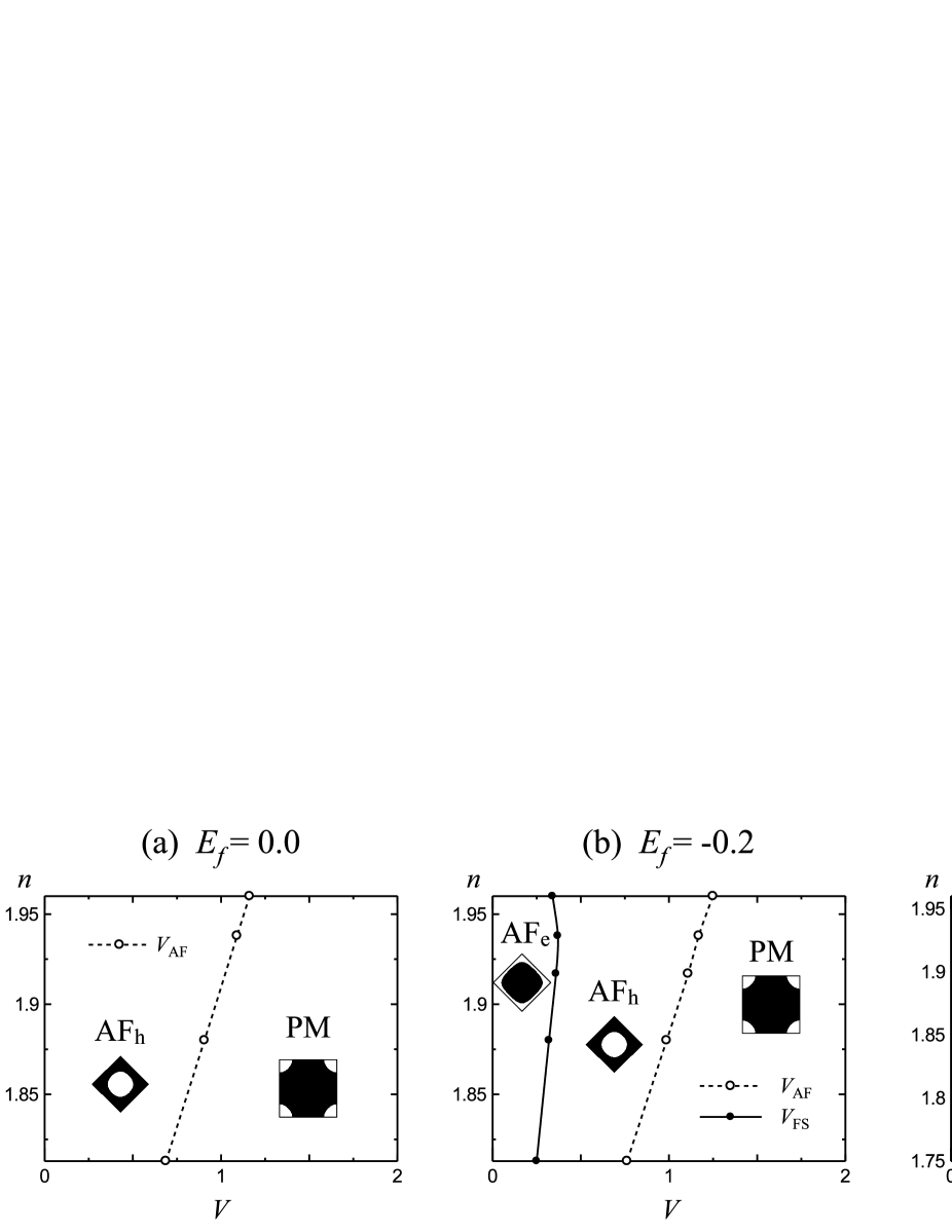
Figure 1: Ground state phase diagram of $U=\infty$ PAM in a two-dimensional square lattice. Solid curves ($V_{\mathrm{FS}}$ and $V_{\mathrm{AF+FS}}$) represent the first-order phase transition and dotted curves ($V_{\mathrm{AF}}$) represent the second-order one.

For fixed values of $E_{f}$ and $n$, the change of the ground state is classified into three cases: (i) PM $\rightarrow$ AF_h, (ii) PM $\rightarrow$ AF_h $\rightarrow$ AF_e and (iii) PM $\rightarrow$ AF_e. In Fig. 2, we show the energy comparison between the trial wave functions for each case and discuss the behaviors of the staggered magnetization of $f$ electrons, $M_{f}=\bigl{<}n^{f}_{\mathrm{A\uparrow}}\bigr{>}-\bigl{<}n^{f}_{\mathrm{A\downarrow}}\bigr{>}=-\bigl{(}\bigl{<}n^{f}_{\mathrm{B\uparrow}}\bigr{>}-\bigl{<}n^{f}_{\mathrm{B\downarrow}}\bigr{>}\bigr{)}$, and the average $f$-electron density $\left<n_{f}\right>$.

Figure 2(a) shows the case of (i) at $E_{f}=0.0$ and $n=1.880$. The ground state is PM for $V>V_{\mathrm{AF}}$ and AF_h for $V<V_{\mathrm{AF}}$. The variational energy of AF_h smoothly merges with that of PM (horizontal axis) at $V=V_{\mathrm{AF}}$, indicating the second-order (continuous) AF transition. $M_{f}$ continuously increases from zero as $V$ decreases from $V_{\mathrm{AF}}$. $\left<n_{f}\right>$ monotonically increases as $V$ decreases from the PM side, and shows continuous change across the AF transition.

The case of (ii) at $E_{f}=-0.2$ and $n=1.880$ is shown in Fig. 2(b). As in the case of (i), the transition from PM to AF_h at $V=V_{\mathrm{AF}}$ is second-order. The changes of $M_{f}$ and $\left<n_{f}\right>$ across the AF transition are continuous. On the other hand, when the Fermi-surface reconstruction (AF_h $\rightarrow$ AF_e) occurs, abrupt changes are observed. At $V=V_{\mathrm{FS}}$, the energy crossing occurs and the ground state changes from AF_h to AF_e. It is clearly a first-order transition and physical quantities such as $M_{f}$ and $\left<n_{f}\right>$ discontinuously increase across the transition. As one can see from Fig. 2(b), the $f$ electrons are almost localized in AF_e and $M_{f}\simeq\left<n_{f}\right>$ is satisfied. It shows that the Kondo screening, which works so as to suppress the AF order, becomes almost irrelevant in AF_e and the local $f$-electron moment is almost fully polarized.

The case of (iii) at $E_{f}=-1.0$ and $n=1.750$ is shown in Fig. 2(c). Contrary to the cases of (i) and (ii), AF_h does not appear for any values of $V$; the variational energy of AF_h is always higher than that of AF_e, and the ground state directly changes from PM to AF_e at $V=V_{\mathrm{AF+FS}}$. It is a first-order transition, where the AF transition and the Fermi-surface reconstruction occur simultaneously. As a result, $M_{f}$ shows discontinuous jump from zero to a finite value at $V=V_{\mathrm{AF+FS}}$. As in the case of (ii), $M_{f}\simeq\left<n_{f}\right>$ is satisfied and the almost fully polarized AF state is realized in AF_e.

Note that AF_S does not appear for all cases. It is a natural result since AF_S cannot gain the mixing energy because of $\tilde{V}=0$ and it is energetically unfavorable under the condition of $V\neq 0$. The introduction of small but finite value of $\tilde{V}$ does not change the shape of the Fermi surface very much, but it leads to a mixing energy gain and stabilizes AF_e. In AF_e, the $c$ electrons enlarge the occupied phase space and become heavy compared with the case of AF_S because of the finite value of $\tilde{V}$. Namely, AF_e and AF_S have almost the same Fermi surface but their internal structures of quasiparticles are completely different.

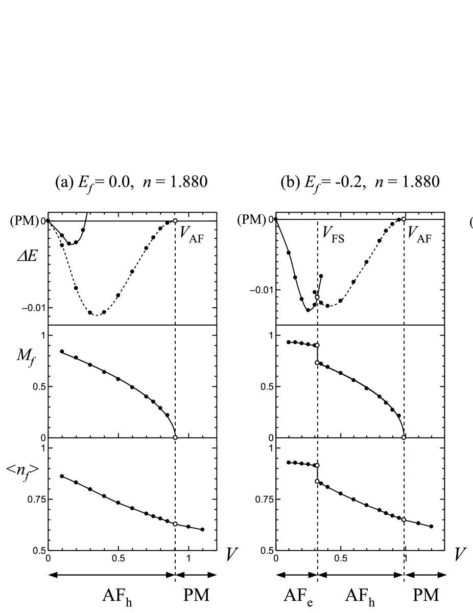
Figure 2: $V$ dependence of condensation energy $\Delta E$, staggered magnetization of $f$ electrons $M_{f}$ and average $f$-electron density $\left<n_{f}\right>$. $\Delta E$ are variational energies of AF_e (solid curves) and AF_h (dotted curves) compared with that of PM. Open circles correspond to the transition points.

3.2 Origin of the Fermi Surface Reconstruction

In §3.1, we have shown the existence of the novel type of quantum phase transition of “Fermi-surface reconstruction”. In this section, we discuss its origin. Figure 3 shows the band dispersions of the three different states obtained by diagonalizing the one-body part $\left|\Phi\right>$ with optimized parameters: PM ($V$=1.50), AF_h ($V$=1.00) and AF_e ($V$=0.70) at $E_{F}=-1.0$ and $n=1.880$. In PM, only the lower hybridized band is shown since the upper one is away from the Fermi energy and unoccupied. In AF_h, the energy band is folded and the AF gap opens along the AF Brillouin zone boundary (($\pi,0$) and ($\pi/2,\pi/2$) in Fig. 3(b)). This folding does not change the topology of the Fermi surface compared with Fig. 3(a). As $V$ decreases in AF_h, the optimized value of $\tilde{V}$ also decreases and that of $\Delta_{f}$ increases. Following the growth of the AF gap, the band dispersion changes in the direction as shown by the arrows in Fig. 3(b) and finally changes into a dispersion which is convex downward. As a result, quasiparticle occupation changes in the $\bm{k}$-space and the Fermi surface is reconstructed from hole-like (AF_h) to electron-like (AF_e) at $V=V_{\mathrm{FS}}$. According to this mechanism, it is in principle possible that the Fermi-surface reconstruction becomes a second-order transition. However, within our trial wave function, the Fermi-surface reconstruction is clearly a first-order transition which accompanies the energy crossing.

Next we discuss the origin of the Fermi-surface reconstruction from a viewpoint of energy gain. The variational parameter $\tilde{V}$ corresponds to the effective hybridization and thus it will be directly related to the degree of Kondo screening. It works so as to gain the mixing energy $E_{\mathrm{mix}}$, the third term in eq.(1). On the other hand, $\Delta_{f}$ corresponds to the AF gap and controls the magnitude of the AF order. It stabilizes the local $f$-electron moment and suppresses the hybridization, leading to gain the kinetic energy of $c$ electrons $E_{\mathrm{kin}}$ and the $f$-electrons energy $E_{n_{f}}$, which are the first and the second terms in eq.(1), respectively. In PM and AF_h, the role of $\tilde{V}$ is dominant and the system forms the hole-like Fermi surface which is favorable for $E_{\mathrm{mix}}$. In AF_e, on the other hand, the role of $\Delta_{f}$ exceeds that of $\tilde{V}$ and the electron-like Fermi surface, which is favorable for $E_{\mathrm{kin}}$ and $E_{n_{f}}$, is formed. Namely, the origin of the Fermi-surface reconstruction is a change of the mechanism of the energy gain. In AF_e, the localization of $f$ electrons is essential for the energy gain and the AF order is considered to be additional. Therefore, the region of AF_e in the phase diagram mainly depends on $E_{f}$, but not so much on the total electron density $n$ which is closely related to the stability of the AF order. It is in contrast to the case of AF_h whose stability greatly depends on $n$.

The existence of the Fermi-surface reconstruction is also suggested in the recent study of the cellular dynamical mean-field theory (CDMFT) by De Leo et al [19]. They have calculated spectral functions for paramagnetic and AF states and shown that the AF transition is accompanied by a dramatic rearrangement of the spectral weight. It suggests the change of the topology of the Fermi surface and can be regarded as a kind of Fermi-surface reconstruction. Although the condition of their calculation is somewhat different with ours (the chemical potential is fixed in ref. Leo instead of the electron density), their result is consistent with the existence of the Fermi-surface reconstruction.

Let us mention here the order of the transition. In our results, the Fermi-surface reconstruction is clearly a first-order transition. However, as mentioned before, it is to be noted that the second-order (or other continuous) transition cannot be completely ruled out since the result depends on the choice of the trial wave functions.

Finally, we compare the present results with the Kondo lattice model (KLM). In the previous paper [17], we have shown that the Fermi-surface reconstruction occurs in the KLM. The result that the Fermi-surface reconstruction occurs for $U=\infty$ and sufficiently low value of $E_{f}$ in the PAM is consistent with the result of the KLM, since the KLM is an effective model of the PAM in the limit of $U\rightarrow\infty$ and $n_{f}\rightarrow 1$. Recent studies of the dynamical cluster approximation [20] and the Gutzwiller approximation [21] also support the existence of the Fermi-surface reconstruction in the KLM. In the Gutzwiller approximation, the one-body part is more improved than ours but the obtained phase diagram is in good agreement with ours. This means that our variational wave functions capture the essence of the AF transition and the Fermi-surface reconstruction in spite of their rather simple forms.

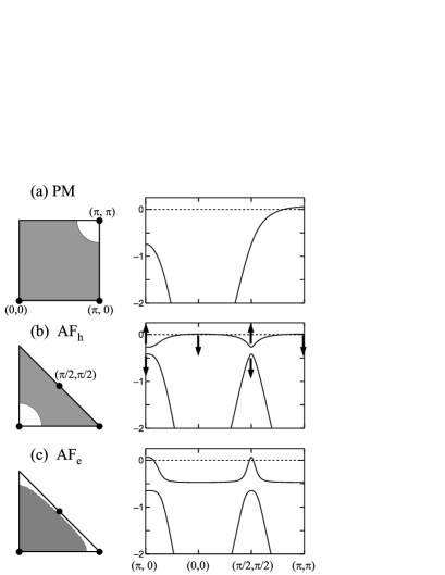
Figure 3: Band dispersions of PM ($V$=1.50), AF_h ($V$=1.00) and AF_e ($V$=0.70) at $E_{F}=-1.0$ and $n=1.880$. The Fermi energy is set to be 0. Arrows indicate the direction of the change of dispersion when $V$ decreases (see text).

3.3 Momentum Distribution Function

So far, we have discussed the Fermi surface obtained from the one-body part $\left|\Phi\right>$ without projection. However, it is in principle possible that the Fermi surface changes by the effect of the projection operator, $P^{f}_{\mathrm{G}}$. Since the Fermi surface is determined from the discontinuities in the momentum distribution function, we calculate them for $c$ and $f$ electrons in this section. They are defined as,

$$n_{c}(\bm{k}) =\frac{1}{2}\sum_{\sigma}\big{<}c^{\dagger}_{\bm{k}\sigma}c_{\bm{k}\sigma}\big{>}=\frac{1}{2N}\sum_{i,j,\sigma}\mathrm{e}^{\mathrm{i}\bm{k}\cdot(\bm{r}_{i}-\bm{r}_{j})}\big{<}c^{\dagger}_{i\sigma}c_{j\sigma}\big{>}$$ (8)

$$n_{f}(\bm{k}) =\frac{1}{2}\sum_{\sigma}\big{<}f^{\dagger}_{\bm{k}\sigma}f_{\bm{k}\sigma}\big{>}=\frac{1}{2N}\sum_{i,j,\sigma}\mathrm{e}^{\mathrm{i}\bm{k}\cdot(\bm{r}_{i}-\bm{r}_{j})}\big{<}f^{\dagger}_{i\sigma}f_{j\sigma}\big{>}.$$ (9)

We calculate $n_{c}(\bm{k})$ and $n_{f}(\bm{k})$ with and without projection, $P^{f}_{G}$, in order to study the role of the projection operator. We set $E_{f}=-1.0$ and $n=n_{c}+n_{f}=612/324=1.889$. Each $\bm{k}$ point is shifted along $y$ direction by $\delta=\pi/9$ because of the antiperiodic boundary condition.

Figure 4 shows the result for PM at $V=1.50$. In PM, the momentum distribution function of $c$ and $f$ electrons without projection are identical to $u_{\bm{k}}^{2}$ (eq.(4)) and $v_{\bm{k}}^{2}$ (eq.(5)). We denote them as $n_{c}^{0}(\bm{k})$ and $n_{f}^{0}(\bm{k})$, respectively. As shown by arrows in Fig. 4(b) and (c), $n_{c}^{0}(\bm{k})$ and $n_{f}^{0}(\bm{k})$ have discontinuities at the same position. Figure 4(a) shows the Fermi surface determined from $n_{c}^{0}(\bm{k})$ and $n_{f}^{0}(\bm{k})$. We call it “original Fermi surface” in the following.

As shown in Fig. 4(b), the projection operator flattens $n_{f}(\bm{k})$ in the whole Brillouin zone and the discontinuities are fairly reduced. Moreover, $n_{f}(\bm{k})$ has finite values even outside the original Fermi surface. They are known as a typical role of the on-site Coulomb interaction $U$. Judging from the $\bm{k}$-dependence of $n_{f}(\bm{k})$ near the original Fermi surface, it is probable that the position of the discontinuities does not change in the presence of $P^{f}_{\mathrm{G}}$. Contrary to $n_{f}(\bm{k})$, $n_{c}(\bm{k})$ is generally enhanced by projection since the excluded $f$ electrons come into the $c$-electron orbital. As shown in Fig. 4(c), the discontinuities in $n_{c}(\bm{k})$ are rather uncertain, but when we fit the data points by polynomials, we find that there are finite jumps at the original Fermi surface. Although it cannot be completely excluded that the discontinuities in $n_{c}(\bm{k})$ disappear, we expect that the original Fermi surface is preserved. If this is the case, we can say that our trial wave function satisfies the Luttinger’s theorem: the volume of the Fermi surface is determined by the electron density and not affected by the strength of electron correlation, unless the phase transition occurs.

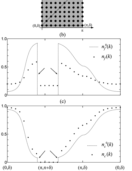
Figure 4: Momentum distribution functions of PM at $E_{F}=-1.0$, $n=1.889$ and $V=1.50$. (a) Occupation of quasiparticles and Fermi surface in the first Brillouin zone. Solid (open) circles represent the occupied (unoccupied) $\bm{k}$-points. Each $\bm{k}$ point is shifted along $y$ direction by $\delta=\pi/9$ because of the antiperiodic boundary condition. Calculated momentum distribution functions of (b) $f$ electrons and (c) $c$ electrons with and without (⁰) projection. Arrows indicate the positions of discontinuities in $n_{f}^{0}(\bm{k})$ and $n_{c}^{0}(\bm{k})$. The optimized variational parameters are $(\tilde{V},\tilde{E_{f}},\Delta_{f},\Delta_{c})=(1.0899,-0.0460,0.0000,0.0000)$

Next we discuss the AF state. As in the case of PM, $n_{c}^{0}(\bm{k})$ and $n_{f}^{0}(\bm{k})$ are explicitly calculated from the one-body part $\left|\Phi\right>$. By diagonalizing the $4\times 4$ matrix in eq.(7), we obtain four quasiparticles ($\alpha_{\bm{k}\sigma},\beta_{\bm{k}\sigma},\gamma_{\bm{k}\sigma},\delta_{\bm{k}\sigma}$) and band dispersions ($E^{\alpha}_{\bm{k}},E^{\beta}_{\bm{k}},E^{\gamma}_{\bm{k}},E^{\delta}_{\bm{k}}$) in the folded AF Brillouin zone. In the present condition, the Fermi energy crosses only the $\beta$-band (see Figs. 3(b) and (c)). The $\alpha$-band is completely filled while the $\gamma$- and the $\delta$-band are empty, i.e., $n^{\alpha}_{\bm{k}}=1$ and $n^{\gamma}_{\bm{k}}=n^{\delta}_{\bm{k}}=0$ for all values of $\bm{k}$. Then $n_{c}^{0}(\bm{k})$ and $n_{f}^{0}(\bm{k})$ are expressed as

$$\begin{cases}\;n_{c}^{0}(\bm{k})&=A_{1}(\bm{k})+\theta(\varepsilon_{\mathrm{F}}-E^{\beta}_{\bm{k}})A_{5}(\bm{k})\\ \;n_{c}^{0}(\bm{k}+\bm{Q})&=A_{2}(\bm{k})+\theta(\varepsilon_{\mathrm{F}}-E^{\beta}_{\bm{k}})A_{6}(\bm{k})\\ \;n_{f}^{0}(\bm{k})&=A_{3}(\bm{k})+\theta(\varepsilon_{\mathrm{F}}-E^{\beta}_{\bm{k}})A_{7}(\bm{k})\\ \;n_{f}^{0}(\bm{k}+\bm{Q})&=A_{4}(\bm{k})+\theta(\varepsilon_{\mathrm{F}}-E^{\beta}_{\bm{k}})A_{8}(\bm{k})\end{cases},$$ (10)

where $\theta(x)$ is the step function and $\varepsilon_{\mathrm{F}}$ denotes the Fermi energy. Here $A_{i}(\bm{k})$ are derived from the eigenvectors obtained in the diagonalization. We can see that the discontinuities in $n_{c}^{0}(\bm{k})$ and $n_{f}^{0}(\bm{k})$ are determined by the occupation of the $\beta$-band.

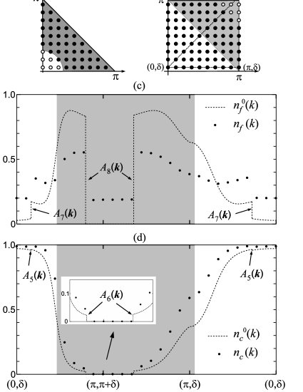
Figure 5: Momentum distribution functions of AF_h at $E_{F}=-1.0$, $n=1.889$ and $V=1.00$. (a) Occupation of quasiparticles in the $\beta$-band and Fermi surface in the folded AF Brillouin zone. Solid (open) circles represent the occupied (unoccupied) $\bm{k}$-points. (b) First Brillouin zone described with the extended zone scheme. Calculated momentum distribution functions of (c) $f$ electrons and (d) $c$ electrons with and without (⁰) projection. Arrows indicate the positions of discontinuities in $n_{f}^{0}(\bm{k})$ and $n_{c}^{0}(\bm{k})$. The optimized variational parameters are $(\tilde{V},\tilde{E_{f}},\Delta_{f},\Delta_{c})=(0.6368,-0.3236,0.1193,0.0000)$

Figure 5 shows the result for AF_h at $V=1.00$. The original Fermi surface determined from $n_{c}^{0}(\bm{k})$ and $n_{f}^{0}(\bm{k})$ is shown in Fig. 5(a). To make the comparison with the case of PM easier, we use the extended Brillouin zone scheme in the following. The shaded areas in Figs. 5(b), (c) and (d) are folded in the reduced Brillouin zone scheme. Compared with the case of PM, additional discontinuities, whose magnitudes are $A_{7}(\bm{k})$, appear in $n_{f}^{0}(\bm{k})$ as shown in Fig. 5(c). It is originated from the appearance of the AF order in $f$ electrons. In the same way, additional discontinuities, whose magnitudes are $A_{5}(\bm{k})$, also appear in $n_{c}^{0}(\bm{k})$, although they are very small.

As shown in Fig. 5(c), $n_{f}(\bm{k})$ is flattened in the whole Brillouin zone by the effect of $P^{f}_{\mathrm{G}}$ as in the case of PM. However, discontinuities originated from $n_{f}^{0}(\bm{k})$ seems to be preserved in $n_{f}(\bm{k})$. The discontinuities in $n_{c}(\bm{k})$ is rather uncertain because of their smallness (see the inset of Fig. 5(d)). However, by fitting the data points by polynomials, we can find a finite jump at the original Fermi surface. In conclusion, we expect that the original Fermi surface is preserved through the projection also in AF_h.

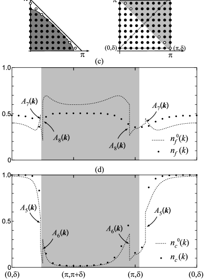
Figure 6: Momentum distribution functions of AF_e at $E_{F}=-1.0$, $n=1.889$ and $V=0.90$. Notation is the same with that of Fig. 5. The optimized variational parameters are $(\tilde{V},\tilde{E_{f}},\Delta_{f},\Delta_{c})=(0.6607,-0.0905,0.4722,0.0000)$

Figure 6 shows the result for AF_e at $V=0.90$. Contrary to the case of PM and AF_h, the result is somewhat different in AF_e. The discontinuities exist near the AF Brillouin zone boundary both in $n_{c}^{0}(\bm{k})$ and $n_{f}^{0}(\bm{k})$ as shown by the arrows in Figs. 6(c) and (d). However, $n_{f}(\bm{k})$ is greatly flattened by projection and the discontinuities are greatly suppressed. If these discontinuities disappear, $f$ electrons become completely localized and do not contribute to the Fermi surface. We cannot say whether the discontinuities in $n_{f}(\bm{k})$ really disappear or not within this calculation. However, it is certain that the itinerancy of $f$ electrons is greatly suppressed in AF_e compared with the case of PM and AF_h. On the other hand, the discontinuities in $n_{c}(\bm{k})$ seems to exist at the original Fermi surface, as in the case of PM and AF_h. In this sense, the volume and the shape of the Fermi surface is preserved through the projection also in AF_e, whichever the discontinuities in $n_{f}(\bm{k})$ disappear or not. This result shows that even if the $f$ electrons do not contribute to the Fermi surface, the $c$ electrons “recognize” the existence of $f$ electrons and preserve the original Fermi surface. It is possible that $c$ electrons are redistributed by the effect of projection and form a “small” Fermi surface whose volume is determined by the number of $c$ electrons alone. If it occurs, the discontinuities in $n_{c}(\bm{k})$ exist only in the unshaded area and the discontinuities in the shaded area must disappear. But this is not the case.

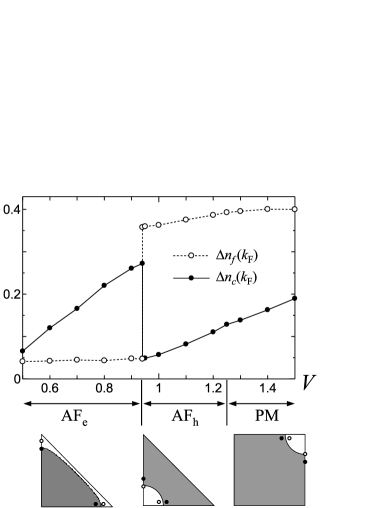
Figure 7: $V$ dependences of the discontinuities of $n_{c}(\bm{k})$ and $n_{f}(\bm{k})$ at the Fermi surface. They are estimated from the average of two directions shown above.

Finally we discuss how much the electrons are correlated and become heavy from the discontinuities in $n_{c}(\bm{k})$ and $n_{f}(\bm{k})$. We estimate the discontinuities at the Fermi surface from the difference between the values just inside and just outside of the Fermi surface. As typical cases, we calculate them along two directions shown in the bottom panels in Fig. 7 and average their values. The upper panel of Fig. 7 shows the obtained $\Delta n_{c}(k_{\mathrm{F}})$ and $\Delta n_{f}(k_{\mathrm{F}})$. In PM and AF_h, $\Delta n_{c}(k_{\mathrm{F}})$ and $\Delta n_{f}(k_{\mathrm{F}})$ continuously decrease as $V$ decreases. When the Fermi-surface reconstruction occurs (AF_h $\rightarrow$ AF_e), a drastic change is observed. $\Delta n_{c}(k_{\mathrm{F}})$ discontinuously increases since the position of $k_{\mathrm{F}}$ shifts near the AF Brillouin zone boundary, where the value of $n_{c}(\bm{k})$ is rather large compared with the former position. It shows that the $c$ electrons recover the weight at the Fermi energy. Note that even after the Fermi-surface reconstruction, $c$ electrons are renormalized compared with the case of AF_S ($\Delta n_{c}(k_{\mathrm{F}})=1$). On the other hand, $\Delta n_{f}(k_{\mathrm{F}})$ discontinuously decreases to a small value through the Fermi-surface reconstruction. It shows that the $f$ electrons become almost localized and their itinerancy is fairly suppressed in AF_e. From these results, we expect that the transition to AF_e is a kind of orbital-selective Mott transition where only the $f$ electrons become localized, as proposed in the CDMFT study [19]. However, as mentioned before, we cannot say whether $\Delta n_{f}(k_{\mathrm{F}})$ becomes zero or not within this calculation. Moreover, the calculation for all directions is necessary for a precise discussion. It is left for an interesting future problem.

4 Discussion

We discuss the relation between our results and the experiments. If the Fermi-surface reconstruction occurs, changes in various physical quantities are expected. The abrupt change of dHvA frequencies across the AF transition shows the appearance of a Fermi surface with different topology [1, 2, 3, 4], indicating the occurrence of a Fermi-surface reconstruction. The picture that the $f$ electrons are localized in the AF phase and are itinerant in the paramagnetic phase, which is proposed from the comparison of dHvA results and the band calculation, is also consistent with the scenario of a Fermi-surface reconstruction.

On the other hand, it have been proposed that the AF transition ($x\sim 0.8$) and the abrupt change of dHvA frequencies ($x\sim 0.4$) are not coincident in CeRh_1-xCo_xIn₅. At $x=0.4$, the magnetic structure changes from incommensurate ($x<0.4$) to commensurate ($x>0.4$) within the AF phase [7]. The fitting with band calculation suggests that the former AF phase corresponds to CeRhIn₅ type (4$f$-localized picture) and the latter corresponds to CeCoIn₅ type (4$f$-itinerant picture). We expect that this transition is closely related to the Fermi-surface reconstruction within the AF phase (AF_e $\rightarrow$ AF_h), although the more realistic calculation is necessary for a precise discussion.

The abrupt change of the Hall coefficient at the AF QCP in YbRh₂Si₂ [5] is also indicative of a Fermi-surface reconstruction. However, the band calculation shows that the Hall coefficient is determined by several contributions with opposite signs and is very sensitive to the energy level of $f$ electrons. It was pointed out that small changes in the $f$-electron occupation are sufficient to reproduce the experimental result [22]. Therefore, we cannot directly related the Fermi-surface reconstruction to the AF QCP in YbRh₂Si₂ at this stage.

We also refer to the effective mass in the AF state. The dHvA experiment shows that the Fermi surface of CeRhIn₅ is quite similar to that of non-4$f$ reference compound of LaRhIn₅ [23]. It suggests that the contribution of the 4$f$ electrons to the Fermi surface is rather small in CeRhIn₅. However, the obtained cyclotron mass in CeRhIn₅ is roughly by one order larger than that in LaRhIn₅ [23]. We consider that the existence of 4$f$ electrons does induce this mass enhancement, keeping the Fermi surface almost unchanged. As we have shown in the case of AF_e, it is possible that $f$ electrons do not contribute to the Fermi surface at all but the $c$ electrons are renormalized and heavy reflecting the existence of the $f$ electrons. It can explain the enhancement of cyclotron mass in CeRhIn₅.

5 Summary

In summary, we have studied the ground state phase diagrams and some physical quantities of the PAM in a two-dimensional square lattice with VMC method. We have shown that

• The Fermi-surface reconstruction which accompanies the localization of $f$ electrons occurs in a wide region of parameters. It induces the topological change of the Fermi surface and stabilizes the localized AF state.

• The conventional itinerant AF transition also occurs separately from the Fermi-surface reconstruction.

• Even in the localized AF state, the $c$ electrons are renormalized compared with the non-interacting case, reflecting the existence of $f$ electrons.

These results will be a good starting point to clarify the relation between the AF transition and the change of the Fermi surface in heavy-fermion systems. For a more detailed discussion, calculations with realistic conditions will be necessary: three dimensional lattice structure, degeneracy of orbitals, magnetic ordering with incommensurate wave vector, and so on. However, we think that the simple model discussed here capture the essence of the Fermi-surface reconstruction, which occurs in general as the evidence of strong localized character of $f$ electrons.

References

- [1] S. Araki, R. Settai, T. C. Kobayashi, H. Harima, and Y. Ōnuki: Phys. Rev. B 64 (2001) 224417.
- [2] R. Settai, T. Kubo, T. Shiromoto, D. Honda, H. Shishido, K. Sugiyama, Y. Haga, T. D. Matsuda, K. Betsuyaku, H. Harima, T. C. Kobayashi, and Y. Ōnuki: J. Phys. Soc. Jpn. 74 (2005) 3016.
- [3] H. Shishido, R. Settai, H. Harima, and Y. Ōnuki: J. Phys. Soc. Jpn. 74 (2005) 1103.
- [4] S. Elgazzar, I. Opahle, R. Hayn, and P. M. Oppenneer: Phys. Rev. B 69 (2004) 214510.
- [5] S. Paschen, T. Lühmann, S. Wirth, P. Gegenwart, O. Trovarelli, C. Geibel, F. Steglich, P. Coleman, and Q. Si: Nature (London) 432 (2004) 881.
- [6] S. Ohira-Kawamura, H. Shishido, A. Yoshida, R. Okazaki, H. Kawano-Furukawa, T. Shibauchi, H. Harima, and Y. Matsuda: Phys. Rev. B 76 (2007) 132507.
- [7] S. K. Goh, J. Paglione, M. Sutherland, E. C. T. O’Farrell, C. Bergemann, T. A. Sayles, and M. B. Maple: Phys. Rev. Lett. 101 (2008) 056402.
- [8] S. Doniach: Physica 91B (1977) 231.
- [9] T. Moriya: Spin Flucutuations in Itinerant Electron Magnets (Springer-Verlag, Berlin, 1985).
- [10] J. A. Hertz: Phys. Rev. B 14 (1976) 1165.
- [11] A. J. Millis: Phys. Rev. B 48 (1993) 7183.
- [12] Q. Si, S. Rabello, K. Ingersent, and J. L. Smith: Nature (London) 413 (2001) 804.
- [13] P. Coleman, C. Pepin, Q. Si, and R. Ramazashvili: J. Phys.: Condens. Matter 13 (2001) R723.
- [14] T. Senthil, S. Sachdev, and M. Vojta: Physica B 359-361 (2005) 9.
- [15] I. Paul, C. Pépin, and M. R. Norman: Phys. Rev. Lett. 98 (2007) 026402.
- [16] C. Pépin: Phys. Rev. Lett. 98 (2007) 206401.
- [17] H. Watanabe and M. Ogata, Phys. Rev. Lett. 99 (2007) 136401.
- [18] H. Shiba, J. Phys. Soc. Jpn. 55 (1986) 2765.
- [19] L. D. Leo, M. Civelli, and G. Kotliar: Phys. Rev. B 77 (2008) 075107.
- [20] L. C. Martin and F. F. Assaad: Phys. Rev. B 101 (2008) 066404.
- [21] N. Lanatà, P. Barone, and M. Fabrizio: arXiv:0807.3849.
- [22] M. R. Norman, Phys. Rev. B 71 (2005) 220405(R).
- [23] H. Shishido, R. Settai, D. Aoki, S. Ikeda, H. Nakawaki, N. Nakamura, T. Iizuka, Y. Inada, K. Sugiyama, T. Takeuchi, K. Kindo, T. C. Kobayashi, Y. Haga, H. Harima, Y. Aoki, T. Namiki, H. Sato, and Y. Ōnuki: J. Phys. Soc. Jpn. 71 (2002) 162.