Two-Impurity Anderson model in an Antiferromagnetic metal: zero-bandwidth limit.

Abstract

We study the zero-bandwidth limit of the two-impurity Anderson model in an antiferromagnetic (AF) metal. We calculate, for different values of the model parameters, the lowest excitation energy, the magnetic correlation $<\mathbf{S}_{1}\mathbf{S}_{2}>$ between the impurities, and the magnetic moment at each impurity site, as a function of the distance between the impurities and the temperature. At zero temperature, in the region of parameters corresponding to the Kondo regime of the impurities, we observe an interesting competition between the AF gap and the Kondo physics of the two impurities. When the impurities are close enough, the AF splitting governs the physics of the system and the local moments of the impurities are frozen, in a state with very strong ferromagnetic correlation between the impurities and roughly independent of the distance. On the contrary, when the impurities are sufficiently far apart and the AF gap is not too large, the scenario of the Kondo physics take place: non-magnetic ground state and the possibility of spin-flip excitation emerges and the ferromagnetic $<\mathbf{S}_{1}\mathbf{S}_{2}>$ decreases as the distance increases, but the complete decoupling of the impurities never occurs. In adition, the presence of the AF gap gives a non-zero magnetic moment at each impurity site, showing a non complete Kondo screening of the impurities in the system. We observe that the residual magnetic moment decreases when the distance between the impurities is increased.

I INTRODUCTION

The behavior of spin correlations in heavy fermion systems is still not completely understood. Lee At high temperatures, heavy fermion materials behave like a collection of individual local moments. When the temperature goes down, correlations take place and the Kondo effectKondo can occur in this systems. This screening can quench the magnetic interaction between local moments and the question is: how can spin polarizations propagate to other local moments. A first approach toward the understanding of this very interesting problem, the competition between Kondo effect and Ruderman-Kittel-Kasuya-Yosida interaction (RKKY)RKKY has been studied in the simplified framework of the two-impurity AndersonAnder2 or KondoKon2 models. Recently, in the Kondo limit, a systematic study of the ground states of two Anderson impurities has been realized.Simonin Both models take into account the conduction electrons in a non-magnetic band. Nevertheless, many experiments in heavy fermion systems show antiferromagnetic correlations or orderings at low temperatures. For example, inelastic neutron scattering from the antiferromagnetic heavy fermion system U₂Zn₁₇Bro shows spin fluctuations in this material. Also, UPt₃Aepp and URu₂Si₂Broh are both heavy fermion compounds where spin fluctuations and antiferromagnetic correlations are present. This suggests that to understand the anomalous properties of these materials, it is necessary to study also the Kondo effect in presence of different kind of magnetic order of itinerant electrons. Zhang and YuZha considered a half-filled anisotropic Kondo lattice model within a mean field theory and found a coexistence of antiferromagnetic long-range order and the Kondo singlet state. Similar results are obtained by Capponi and AssaadCap using a Quantum Monte Carlo algorithm. Recently, the single Kondo effect in an antiferromagnetic metal was studied.Aji This work shows that for a general location of the impurity, the Kondo singularities still occur, but the ground state has a partially unscreened moment. From the theoretical point of view, a natural extension of this problem is to consider the case of two-magnetic impurities in an antiferromagnetic metal. The study of a pair of spin-1/2 impurities is a starting point for our understanding of a lattice behavior in this kind of materials. The aim of this work is to present a very simple approach to study how the competition between partial quenching of the individual moments and their indirect interaction via the antiferromagnetic conduction electrons take place. To this end, as a first approach to the solution of this problem, we extend the zero band-width (ZBW) limit approximation of the two-impurity Anderson model in a paramagnetic metalAllub , to include the AF conduction band.Aji Despite our simple approximation, the ZBW limit has been successfully applied to explain qualitatively most of the experimental results in valence fluctuating problems.angost This limit also gives a good description of the magnetic reentrance phenomena in superconductors with Kondo impurities.reentr Also this method was applied to explain transport experiments on semiconductor quantum dots.Allu An attractive feature of the ZBW limit, is that all calculations can be realized exactly with a minimum of numerical effort and the results are very satisfying, since they reproduce results for properties found much more laboriously by other techniques. For example, the most important results of our previous paperAllub were obtained in Ref.Simonin by means of variational wave functions. Nevertheless, it is important to recognize that the ZBW limit is oversimplified, specifically in not containing any band structures and consequently we must expect to obtain a cartoon of the real picture. In summary, motivated by the experimental results in the magnetic heavy fermion systems as mentioned above and by the previous successful theoretical work and following this track of thought, we employ the ZBW limit to study this very interesting problem. In absence of more elaborated theoretical solutions, this approach often gives results in a good qualitative agreement with experimental data.

We introduce the two-impurity Anderson Hamiltonian and set up the zero band-width approximation to this problem in Section 2. Section 3 is devoted to present the numerical results and discusses their physical implications. Section 4 is devoted to conclusions.

II MODEL

We start from the two-impurity Anderson HamiltonianAnderso in the absence of direct hopping between impurities extended to include the antiferromagnetism of the itinerant electrons:

$$H = \sum_{\mathbf{k},\sigma}\varepsilon_{(\mathbf{k)}}\text{ }c_{\mathbf{k}\sigma}^{\dagger}c_{\mathbf{k}\sigma}+\sum_{\mathbf{k}}[\Gamma\text{ }(c_{\mathbf{k}\uparrow}^{\dagger}c_{\mathbf{k+Q}\uparrow}-c_{\mathbf{k}\downarrow}^{\dagger}c_{\mathbf{k+Q}\downarrow})+\text{H.c.}]$$ (1)

$$+\varepsilon_{d}\sum_{\sigma,j=1,2}\text{ }d_{j\sigma}^{\dagger}d_{j\sigma}+U\sum_{j=1,2}\text{ }d_{j\uparrow}^{\dagger}d_{j\uparrow}d_{j\downarrow}^{\dagger}d_{j\downarrow}$$

$$+\sum_{\mathbf{k},\sigma,j=1,2}V_{kj}\text{ }(c_{\mathbf{k}\sigma}^{\dagger}d_{j\sigma}\,+\text{H.c.}),$$

where $c_{\mathbf{k}\sigma}^{\dagger}$ ($c_{\mathbf{k}\sigma}$) creates (destroys) an electron with momentum $\mathbf{k}$ and spin $\sigma$ in the conduction band with energy $\varepsilon_{(\mathbf{k)}}$, and $d_{j\sigma}^{\dagger}$ ($d_{j\sigma}$) creates (destroys) a localized electron with spin $\sigma$ on the site $\mathbf{R}_{j}$ with energy $\varepsilon_{d}$. Besides, $\Gamma$ is the AF gap, $\mathbf{Q}$ is the ordering wave-vector, $U$ is the localized-orbital Coulomb interaction, and $V_{kj}=Ve^{i\mathbf{k\cdot R}_{j}}$ where $V$ is the hybridization strength. For $\Gamma=0$, $H$ reduces to the well-known two-impurity Anderson modelAnderso . From the practical point of view, the ZBW approximation replaces the structureless conduction bands by few states, located just at the Fermi energy ($\varepsilon_{F}$); conceptually, this recognizes the fact that in most experiments essentially only levels close to the Fermi energy are relevant. As in the previous paper,Allub we take here two different vectors $\mathbf{k}$ ($\mathbf{k}_{1}$ and $\mathbf{k}_{2}$ with $\mathbf{k}_{1}\neq\mathbf{k}_{2}$ and $|\mathbf{k}_{1}|=|\mathbf{k}_{2}|=|\mathbf{k}_{F}|$, with $\mathbf{k}_{F}$ the Fermi momentum) as a minimal model to compensate the two localized spins at the impurities sites. The model should lead to two independent Anderson problems when the impurities are sufficiently far apart and $\Gamma=0$. Accordingly, the original Hamiltonian of Eq. (1) reduces to

$$H_{ZBW} = \varepsilon_{F}\sum_{\sigma}\text{ }(c_{k_{1}\sigma}^{\dagger}c_{k_{1}\sigma}+c_{k_{2}\sigma}^{\dagger}c_{k_{2}\sigma})$$ (2)

$$+\Gamma\text{ }[(c_{k_{1}\uparrow}^{\dagger}c_{k_{2}\uparrow}-c_{k_{1}\downarrow}^{\dagger}c_{k_{2}\downarrow})+\text{H.c.}]$$

$$+\varepsilon_{d}\sum_{\sigma,j=1,2}\text{ }d_{j\sigma}^{\dagger}d_{j\sigma}+U\sum_{j=1,2}\text{ }d_{j\uparrow}^{\dagger}d_{j\uparrow}d_{j\downarrow}^{\dagger}d_{j\downarrow}$$

$$+V\sum_{\sigma}(e^{i\phi_{1}}\text{ }c_{k_{1}\sigma}^{\dagger}d_{1\sigma}\,+e^{i\phi_{1}^{\prime}}\text{ }c_{k_{2}\sigma}^{\dagger}d_{1\sigma}$$

$$+e^{i\phi_{2}^{\prime}}\text{ }c_{k_{1}\sigma}^{\dagger}d_{2\sigma}\,+e^{i\phi_{2}}\text{ }c_{k_{2}\sigma}^{\dagger}d_{2\sigma}+\text{H.c.}),$$

with $k_{1}=|\mathbf{k}_{1}|=|\mathbf{k}_{F}|$, $k_{2}=|\mathbf{k}_{2}|=|\mathbf{k}_{1}+\mathbf{Q}|=|\mathbf{k}_{F}|$, $\phi_{1}=\mathbf{k}_{1}\mathbf{\cdot R}_{1}=\mathbf{k}_{1}\mathbf{\cdot(R}_{2}+\mathbf{r})$, $\phi_{1}^{\prime}=\mathbf{k}_{2}\mathbf{\cdot R}_{1}$,$\phi_{2}^{\prime}=\mathbf{k}_{1}\mathbf{\cdot R}_{2}$, and $\phi_{2}=\mathbf{k}_{2}\mathbf{\cdot R}_{2}=\mathbf{k}_{2}\mathbf{\cdot(R}_{1}-\mathbf{r})$, where $\mathbf{r=R_{1}-R}_{2}$ is the distance between impurities. We can rewrite the Eq. (2) in terms of $\mathbf{r}$, to this end we define $c_{1\sigma}^{\dagger}=$ $e^{i\phi_{2}^{\prime}}c_{k_{1}\sigma}^{\dagger}$ and $c_{2\sigma}^{\dagger}=$ $e^{i\phi_{1}^{\prime}}c_{k_{2}\sigma}^{\dagger}$:

$$H_{ZBW} = \varepsilon_{F}\sum_{\sigma}\text{ }(c_{1\sigma}^{\dagger}c_{1\sigma}+c_{2\sigma}^{\dagger}c_{2\sigma})$$ (3)

$$+\Gamma\text{ }[e^{-i(\mathbf{k}_{1}\mathbf{\cdot R_{2}}-\mathbf{k}_{2}\mathbf{\cdot R_{1}})}(c_{1\uparrow}^{\dagger}c_{2\uparrow}-c_{1\downarrow}^{\dagger}c_{2\downarrow})+\text{H.c.}]$$

$$+\varepsilon_{d}\sum_{\sigma,j=1,2}\text{ }d_{j\sigma}^{\dagger}d_{j\sigma}+U\sum_{j=1,2}\text{ }d_{j\uparrow}^{\dagger}d_{j\uparrow}d_{j\downarrow}^{\dagger}d_{j\downarrow}$$

$$+V\sum_{\sigma}(e^{i\mathbf{k}_{1}\mathbf{\cdot r}}\text{ }c_{1\sigma}^{\dagger}d_{1\sigma}\,+c_{2\sigma}^{\dagger}d_{1\sigma}$$

$$+c_{1\sigma}^{\dagger}d_{2\sigma}\,+e^{-i\mathbf{k}_{2}\mathbf{\cdot r}}\text{ }c_{2\sigma}^{\dagger}d_{2\sigma}+\text{H.c.}),$$

To solve the model Hamiltonian with a minimal number of parameters we take $\mathbf{R}_{1}=\mathbf{r}/2$ and $\mathbf{R}_{2}=-\mathbf{r}/2$, and we define $\phi=\mathbf{k}_{1}\mathbf{\cdot r}$ and $\phi^{\prime}=\mathbf{Q}\mathbf{\cdot r}$. Then, we rewrite Eq.(3) as

$$H_{ZBW} = \varepsilon_{F}\sum_{\sigma}\text{ }(c_{1\sigma}^{\dagger}c_{1\sigma}+c_{2\sigma}^{\dagger}c_{2\sigma})$$ (4)

$$+\Gamma\text{ }[e^{i(\phi+\phi^{\prime}/2)}(c_{1\uparrow}^{\dagger}c_{2\uparrow}-c_{1\downarrow}^{\dagger}c_{2\downarrow})+\text{H.c.}]$$

$$+\varepsilon_{d}\sum_{\sigma,j=1,2}\text{ }d_{j\sigma}^{\dagger}d_{j\sigma}+U\sum_{j=1,2}\text{ }d_{j\uparrow}^{\dagger}d_{j\uparrow}d_{j\downarrow}^{\dagger}d_{j\downarrow}$$

$$+V\sum_{\sigma}(e^{i\phi}\text{ }c_{1\sigma}^{\dagger}d_{1\sigma}\,+c_{2\sigma}^{\dagger}d_{1\sigma}$$

$$+c_{1\sigma}^{\dagger}d_{2\sigma}\,+e^{-i(\phi+\phi^{\prime})}\text{ }c_{2\sigma}^{\dagger}d_{2\sigma}+\text{H.c.}),$$

where we use $\mathbf{k}_{2}\mathbf{\cdot r}=(\mathbf{k}_{1}+\mathbf{Q})\mathbf{\cdot r}=(\phi+\phi^{\prime})$ and $\mathbf{k}_{1}\mathbf{\cdot R_{2}}-\mathbf{k}_{2}\mathbf{\cdot R_{1}}=-[\mathbf{k}_{1}\mathbf{\cdot r}+(\mathbf{k}_{1}+\mathbf{{Q})\cdot r]/2=-(\phi+\phi^{\prime}/2)}$. For $r\rightarrow 0$, $\phi\rightarrow 0$ and $\phi^{\prime}\rightarrow 0$, and we can write the model Hamiltonian as $H_{ZBW}=H_{0}+H_{1}$, with

$$H_{0} = \sum_{\sigma}(\varepsilon_{F}+S_{\sigma}\Gamma)\text{ }\alpha_{1\sigma}^{\dagger}\alpha_{1\sigma}+\varepsilon_{d}\sum_{\sigma,j=1,2}\text{ }d_{j\sigma}^{\dagger}d_{j\sigma}$$ (5)

$$+U\sum_{j=1,2}\text{ }d_{j\uparrow}^{\dagger}d_{j\uparrow}d_{j\downarrow}^{\dagger}d_{j\downarrow}$$

$$+\sqrt{2}V\sum_{\sigma}(\alpha_{1\sigma}^{\dagger}d_{1\sigma}\,+\alpha_{1\sigma}^{\dagger}d_{2\sigma}+\text{H.c.})$$

and

$$H_{1}=\sum_{\sigma}(\varepsilon_{F}-S_{\sigma}\Gamma)\text{ }\alpha_{2\sigma}^{\dagger}\alpha_{2\sigma},$$ (6)

where we define $S_{\sigma}=+$ $(-)$ for the spin $\sigma=\uparrow$ $(\downarrow)$, $\alpha_{1\sigma}^{\dagger}=(c_{1\sigma}^{\dagger}+c_{2\sigma}^{\dagger})/\sqrt{2}$ and $\alpha_{2\sigma}^{\dagger}=(c_{1\sigma}^{\dagger}-c_{2\sigma}^{\dagger})/\sqrt{2}$. This is the limit to the case in which the impurities are close together and we see that the hybridization with the conduction band electrons reduces to only one orbital ($\alpha_{1\sigma}$ )and favors the ferromagnetic coupling between the impurities. So that, the $H_{ZBW}$ reduces to an effective simplified zero band-width Hamiltonian ($H_{0}$) plus a diagonal term ($H_{1}$) disconnected from it. In consequence, the mathematical problem reduces to solve $H_{0}.$ For $\phi\neq 0$ and $\phi^{\prime}=\pm\pi,\pm 3\pi,...,\pm(2n+1)\pi$ the hybridization term reduces to the case in which two orthogonal band states are coupled each to a different impurity (i.e. $V\sum_{\sigma}[(e^{i\phi}c_{1\sigma}^{\dagger}\,+c_{2\sigma}^{\dagger})d_{1\sigma}+(c_{1\sigma}^{\dagger}\,-e^{-i\phi}c_{2\sigma}^{\dagger})d_{2\sigma}\,+$ H.c.$]=\sqrt{2}V\sum_{\sigma}[\gamma_{1\sigma}^{\dagger}d_{1\sigma}+\gamma_{2\sigma}^{\dagger}d_{2\sigma}\,+$ H.c.$]$, where $\gamma_{1\sigma}^{\dagger}=(e^{i\phi}c_{1\sigma}^{\dagger}+c_{2\sigma}^{\dagger})/\sqrt{2}$ and $\gamma_{2\sigma}^{\dagger}=(c_{1\sigma}^{\dagger}-e^{-i\phi}c_{2\sigma}^{\dagger})/\sqrt{2}$). For $\Gamma=0$, this is the limit of the model when the impurities are sufficiently far apart and the ZBW Hamiltonian reduces to two independent Anderson problems. For $\Gamma\neq 0$ and $\phi^{\prime}=\pm\pi$ the antiferromagnetic term reduces to $\Gamma\text{ }[e^{i(\phi+\phi^{\prime}/2)}(c_{1\uparrow}^{\dagger}c_{2\uparrow}-c_{1\downarrow}^{\dagger}c_{2\downarrow})+\text{H.c.}]=\Gamma\text{ }[\mp ie^{-i\phi}(\gamma_{1\uparrow}^{\dagger}\gamma_{2\uparrow}-\gamma_{1\downarrow}^{\dagger}\gamma_{2\downarrow})+\text{H.c.}]$. Therefore, for any value of $\phi$, we can see that the impurities are always correlated due to the antiferromagnetic order of the itinerant electrons. To study the interplay between the hybridization and the antiferromagnetic order in this simple theoretical picture we take hereafter the ordering wave-vector $\mathbf{Q}=-2\mathbf{k}_{1}$ ($\phi^{\prime}=-2\phi$), no different physical results are obtained with other values. So that, Eq. (4) reduces to

$$H_{ZBW} = \varepsilon_{F}\sum_{\sigma}\text{ }(c_{1\sigma}^{\dagger}c_{1\sigma}+c_{2\sigma}^{\dagger}c_{2\sigma})$$ (7)

$$+\Gamma\text{ }[(c_{1\uparrow}^{\dagger}c_{2\uparrow}-c_{1\downarrow}^{\dagger}c_{2\downarrow})+\text{H.c.}]$$

$$+\varepsilon_{d}\sum_{\sigma,j=1,2}\text{ }d_{j\sigma}^{\dagger}d_{j\sigma}+U\sum_{j=1,2}\text{ }d_{j\uparrow}^{\dagger}d_{j\uparrow}d_{j\downarrow}^{\dagger}d_{j\downarrow}$$

$$+V\sum_{\sigma}(e^{i\phi}\text{ }c_{1\sigma}^{\dagger}d_{1\sigma}\,+c_{2\sigma}^{\dagger}d_{1\sigma}$$

$$+c_{1\sigma}^{\dagger}d_{2\sigma}\,+e^{i\phi}\text{ }c_{2\sigma}^{\dagger}d_{2\sigma}+\text{H.c.}).$$

For $\phi=0$ Eq.(7) gives $H_{ZBW}=H_{0}+H_{1}$. For $\phi=\pi/2$ we have $\gamma_{1\sigma}^{\dagger}=(ic_{1\sigma}^{\dagger}+c_{2\sigma}^{\dagger})/\sqrt{2}$ and $\gamma_{2\sigma}^{\dagger}=(c_{1\sigma}^{\dagger}+ic_{2\sigma}^{\dagger})/\sqrt{2}$ and we can rewrite $H_{ZBW}$ in terms of two independent Anderson Hamiltonians plus a coupling term: $H_{ZBW}=H_{A1}+H_{A2}+\Gamma\text{ }[(\gamma_{1\uparrow}^{\dagger}\gamma_{2\uparrow}-\gamma_{1\downarrow}^{\dagger}\gamma_{2\downarrow})+\text{H.c.}]$, where we define

$$H_{Aj} = \varepsilon_{F}\sum_{\sigma}\text{ }\gamma_{j\sigma}^{\dagger}\gamma_{j\sigma}+\varepsilon_{d}\sum_{\sigma}\text{ }d_{j\sigma}^{\dagger}d_{j\sigma}+U\text{ }d_{j\uparrow}^{\dagger}d_{j\uparrow}d_{j\downarrow}^{\dagger}d_{j\downarrow}$$ (8)

$$+\sqrt{2}V\sum_{\sigma}(\gamma_{j\sigma}^{\dagger}d_{j\sigma}\,+\text{H.c.}).$$

III RESULTS AND DISCUSSION

The magnetic correlations between the impurities given by the model Hamiltonian (Eq.7) can be obtained from the four-particle states (this is the most relevant Hilbert space in relation to the two Anderson problems discussed here) or from the grand canonical ensemble adjusting the chemical potential in such a way that the mean total number of particles is always four. There is little numerical difference between these alternative calculations.angost So that, in all the numerical results presented below, we use the four-particle states ($N=4$). For this case, the full Hamiltonian matrix is 70$\times$70. Nevertheless, the solution of the problem reduces to the diagonalization of two 16$\times$16 matrices (for $S_{z}=\pm 1$) and 36$\times$36 matrix (for $S_{z}=0$) as the full Hilbert space is block diagonalized, with each block corresponding to a given $S_{z}$-component. For $S_{z}=\pm 2$, the model gives two degenerate eigenvalues ($\lambda_{2}=2(\varepsilon_{F}+\varepsilon_{d})$). To obtain the numerical results we take the Fermi energy $\varepsilon_{F}=0$ and $V$ as the unit of energy. Therefore, the model is completely characterized by $\varepsilon_{d}$, $U$, $\Gamma$ and the parameter $\phi$ as a measure of the distance between the impurities. We start by presenting in Fig. 1 the energy difference of the two lowest energy levels $E_{K}=(\lambda_{S_{z}=+1}-\lambda_{S_{z}=0})$ as a function of $\phi$, for $\varepsilon_{d}/V=-5$, five different values of $\Gamma/V=$ 0, 0.2, 0.5, 1, and 2, and three different values of $U/V=$ 30, 10, and 5 (Fig. 1(a), (b), and (c)respectively) ranging from the Kondo limit ($U>>|\varepsilon_{d}-\varepsilon_{F}|$) to the intermediate valence (I.V.) regime ($U\sim|\varepsilon_{d}-\varepsilon_{F}|$). We can see that $E_{K}$ always decreases when $\phi$ decreases and also $E_{K}$ decreases when $\Gamma$ is increases. In the Kondo limit (Fig. 1(a)and (b)), for any value $\Gamma/V\neq 0$, $E_{K}<0$ for $\phi=0$ and $E_{K}>0$ for $\phi=\pi/2$. Therefore, for $\Gamma\neq 0$, there is a particular value $\phi=\phi_{c}$, with $0<\phi_{c}<\pi/2$, where $E_{K}=0$. For $\phi<\phi_{c}$ the ground state properties correspond to $S_{z}=+1$ state (if $\Gamma<0$, $S_{z}=-1$) and for $\phi>\phi_{c}$ the $S_{z}=0$ ground state properties take place. In the I.V. regime (Fig. 1(c)), for a given value of $U/|\varepsilon_{d}-\varepsilon_{F}|$, the existence or not of $\phi_{c}$ depend on the value of $\Gamma/V$. When $U/V$ reduces, large values of $\Gamma/V$ are needed to obtain $S_{z}=+1$ ground state at $\phi=0$.

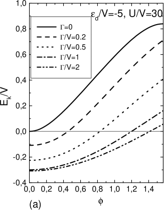
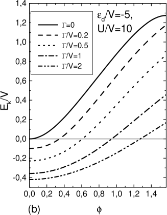
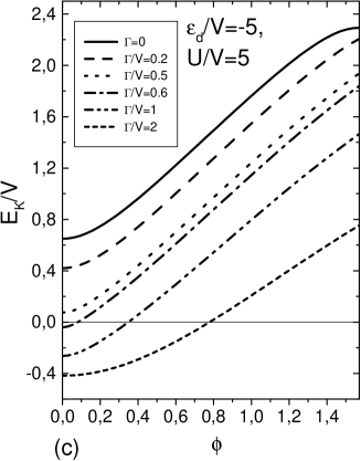
Figure 1: The energy difference $E_{K}=(\lambda_{S_{z}=+1}-\lambda_{S_{z}=0})$ as a function of $\phi$, for $\varepsilon_{d}/V=-5$, five different values of $\Gamma/V=$ 0, 0.2, 0.5, 1, and 2, and three different values of $U/V=$ 30 (a), 10 (b), and 5 (c)

To analyze these results, we consider first the limit of $\phi=\pi/2$, where we have the Hamiltonian $H_{ZBW}=H_{A1}+H_{A2}+\Gamma\text{ }[(\gamma_{1\uparrow}^{\dagger}\gamma_{2\uparrow}-\gamma_{1\downarrow}^{\dagger}\gamma_{2\downarrow})+\text{H.c.}]$. For any value of $\Gamma$, the solution gives $S_{z}=0$ ground state. Therefore, in this limit we have always $E_{K}>0$ (see Fig. 1). It is easy to show this fact in the Kondo limit of each impurity ($U/|\Delta|\rightarrow\infty$, $V/|\Delta|<<1$, with $\Delta=(\varepsilon_{d}-\varepsilon_{F})/2$). In this limit, the 36$\times$36 matrix can be simplified to obtain, approximately, the ground state energy of $H_{ZBW}$ and the corresponding eigenvector ($a_{1},a_{2}$, and $a_{3}$) from the lowest eigenvalue $\lambda_{4,0}$ of the 3x3 matrix given by

$$\hskip 28.45274pt\left|\begin{array}[]{ccc}2\varepsilon_{d}+2J&\Gamma&0\\ \Gamma&2\varepsilon_{d}+J/2&-\sqrt{3}\Gamma\\ 0&-\sqrt{3}\Gamma&2\varepsilon_{d}\end{array}\right|,$$ (9)

with $J=-2V^{2}/|\Delta|$. To this case the ground state reads ($|N,S_{z}>_{\phi}$): $|4,0>_{\pi/2}=\sum_{i}a_{i}|gi>$, where we define $|g1>=\frac{1}{2}[-\gamma_{1\uparrow}^{\dagger}\gamma_{2\uparrow}^{\dagger}|->-\gamma_{1\downarrow}^{\dagger}\gamma_{2\downarrow}^{\dagger}|+>+\frac{1}{\sqrt{2}}(\gamma_{1\uparrow}^{\dagger}\gamma_{2\downarrow}^{\dagger}+\gamma_{1\downarrow}^{\dagger}\gamma_{2\uparrow}^{\dagger})|\Theta>-\frac{1}{\sqrt{2}}(\gamma_{1\uparrow}^{\dagger}\gamma_{2\downarrow}^{\dagger}-\gamma_{1\downarrow}^{\dagger}\gamma_{2\uparrow}^{\dagger})|\Omega>]$, $|g2>=\frac{1}{\sqrt{2}}(\gamma_{2\uparrow}^{\dagger}\gamma_{2\downarrow}^{\dagger}-\gamma_{1\uparrow}^{\dagger}\gamma_{1\downarrow}^{\dagger})|\Theta>$, and $|g3>=\frac{(-1)}{2\sqrt{3}}[\gamma_{1\uparrow}^{\dagger}\gamma_{2\uparrow}^{\dagger}|->+\gamma_{1\downarrow}^{\dagger}\gamma_{2\downarrow}^{\dagger}|+>+3\frac{1}{\sqrt{2}}(\gamma_{1\uparrow}^{\dagger}\gamma_{2\downarrow}^{\dagger}+\gamma_{1\downarrow}^{\dagger}\gamma_{2\uparrow}^{\dagger})|\Theta>+\frac{1}{\sqrt{2}}(\gamma_{1\uparrow}^{\dagger}\gamma_{2\downarrow}^{\dagger}-\gamma_{1\downarrow}^{\dagger}\gamma_{2\uparrow}^{\dagger})|\Omega>]$, with $|+>=d_{1\uparrow}^{\dagger}d_{2\uparrow}^{\dagger}|0>$, $|->=d_{1\downarrow}^{\dagger}d_{2\downarrow}^{\dagger}|0>$, $|\Theta>=\frac{1}{\sqrt{2}}(d_{1\uparrow}^{\dagger}d_{2\downarrow}^{\dagger}+d_{1\downarrow}^{\dagger}d_{2\uparrow}^{\dagger})|0>$, and $|\Omega>=\frac{1}{\sqrt{2}}(d_{1\uparrow}^{\dagger}d_{2\downarrow}^{\dagger}-d_{1\downarrow}^{\dagger}d_{2\uparrow}^{\dagger})|0>$. Note that, $|g1>$ is the product of the two Kondo (one for each impurity) singlet states: $\frac{1}{\sqrt{2}}(\gamma_{1\uparrow}^{\dagger}d_{1\downarrow}^{\dagger}-\gamma_{1\downarrow}^{\dagger}d_{1\uparrow}^{\dagger})*\frac{1}{\sqrt{2}}(\gamma_{2\uparrow}^{\dagger}d_{2\downarrow}^{\dagger}-\gamma_{2\downarrow}^{\dagger}d_{2\uparrow}^{\dagger})|0>$. The explicit form of $|4,0>_{\pi/2}$ shows clearly the important contribution of the ferromagnetic correlations between the impurities in the ground state. Solving the cubic equation we obtain the ground state energy. We can write, approximately, two limiting cases: $\lambda_{4,0}\simeq 2\varepsilon_{d}-2\Gamma+\frac{J}{2}-\frac{3}{16}\frac{J^{2}}{\Gamma}$ for $\Gamma\gg|J|$ and $\lambda_{4,0}\simeq 2\varepsilon_{d}+2J-\frac{2}{3}\frac{\Gamma^{2}}{|J|}$ for $|J|\gg\Gamma$. In a similar manner, the simplification of the 16$\times$16 matrices (for $S_{z}=\pm 1$) in the Kondo limit, allow us to obtain the first excited energy level from the 3$\times$3 matrix given by

$$\hskip 28.45274pt\left|\begin{array}[]{ccc}2\varepsilon_{d}+J&\sqrt{2}\Gamma&0\\ \sqrt{2}\Gamma&2\varepsilon_{d}+J/2&\sqrt{2}\Gamma\\ 0&\sqrt{2}\Gamma&2\varepsilon_{d}\end{array}\right|.$$ (10)

The lowest eigenvalue gives $\lambda_{4,1}=2\varepsilon_{d}+\frac{J}{2}-\sqrt{(\frac{J}{2})^{2}+4\Gamma^{2}}$. Therefore, for $\Gamma>0$ and $\phi=\pi/2$ we obtain, approximately, $E_{K}\simeq\frac{J^{2}}{8\Gamma}$ for $\Gamma\gg|J|$ and $E_{K}\simeq-J-\frac{10}{3}\frac{\Gamma^{2}}{|J|}$ for $|J|\gg\Gamma$. For $\Gamma=0$ (solid lines in Fig. 1(a) and (b)), the problem reduces to solve the one impurity problem ($H_{Aj}$) and we have obtainedAllub $E_{K}=\Delta+R_{0}$, with $R_{0}=\sqrt{\Delta^{2}+4V^{2}}$.

In the opposite limit, for $\phi=0$, the model gives $H_{ZBW}=H_{0}+H_{1}$ and we find that two different ground states are possible:

A) For large Coulomb repulsion ($|\varepsilon_{d}-\varepsilon_{F}|<<U$), the three-particle states and $S_{z}=+1/2$ (for $\Gamma>0$), gives the ground state energy of $H_{0}$ and the corresponding eigenvector ($b_{1},b_{2},b_{3},b_{4}$, and $b_{5}$) can be obtained easily from the lowest eigenvalue $\lambda_{3,+1/2}$ of the 5x5 matrix given by

$$\hskip 28.45274pt\left|\begin{array}[]{ccccc}\varepsilon_{1}-\Gamma&0&2V&0&-2V\\ 0&\varepsilon_{1}+\Gamma&-\sqrt{2}V&0&\sqrt{2}V\\ 2V&-\sqrt{2}V&\varepsilon_{2}&-\sqrt{2}V&0\\ 0&0&-\sqrt{2}V&\varepsilon_{3}+\Gamma&\sqrt{2}V\\ -2V&\sqrt{2}V&0&\sqrt{2}V&\varepsilon_{4}\end{array}\right|,$$ (11)

where $\varepsilon_{1}=2\varepsilon_{d}+\varepsilon_{F}$, $\varepsilon_{2}=\varepsilon_{d}+2\varepsilon_{F}$, $\varepsilon_{3}=2\varepsilon_{d}+\varepsilon_{F}+U$, and $\varepsilon_{4}=3\varepsilon_{d}+U$. So that, the ground state of $H_{0}$ can be written as: $|3,+1/2>_{0}=\sum_{i}b_{i}|hi>$, where we define $|h1>=\alpha_{1\downarrow}^{\dagger}|+>$, $|h2>=\alpha_{1\uparrow}^{\dagger}|\Theta>$, $|h3>=\frac{1}{\sqrt{2}}\alpha_{1\uparrow}^{\dagger}\alpha_{1\downarrow}^{\dagger}(d_{1\uparrow}^{\dagger}-d_{2\uparrow}^{\dagger})|0>$ , $|h4>=\frac{1}{\sqrt{2}}\alpha_{1\uparrow}^{\dagger}(d_{1\uparrow}^{\dagger}d_{1\downarrow}^{\dagger}-d_{2\uparrow}^{\dagger}d_{2\downarrow}^{\dagger})|0>$, and $|h5>=\frac{1}{\sqrt{2}}(d_{1\uparrow}^{\dagger}d_{1\downarrow}^{\dagger}d_{2\uparrow}^{\dagger}-d_{1\uparrow}^{\dagger}d_{2\uparrow}^{\dagger}d_{2\downarrow}^{\dagger})|0>.$ In a similar manner, we obtain the first excited state as $|3,-1/2>_{0}=\sum_{i}b_{i}^{\prime}|h^{\prime}i>$, where $|h^{\prime}1>=\alpha_{1\uparrow}^{\dagger}|->$, $|h^{\prime}2>=\alpha_{1\downarrow}^{\dagger}|\Theta>$, $|h^{\prime}3>=\frac{1}{\sqrt{2}}\alpha_{1\uparrow}^{\dagger}\alpha_{1\downarrow}^{\dagger}(d_{1\downarrow}^{\dagger}-d_{2\downarrow}^{\dagger})|0>$ , $|h^{\prime}4>=\frac{1}{\sqrt{2}}\alpha_{1\downarrow}^{\dagger}(d_{1\uparrow}^{\dagger}d_{1\downarrow}^{\dagger}-d_{2\uparrow}^{\dagger}d_{2\downarrow}^{\dagger})|0>$, and $|h^{\prime}5>=\frac{1}{\sqrt{2}}(d_{1\uparrow}^{\dagger}d_{1\downarrow}^{\dagger}d_{2\downarrow}^{\dagger}-d_{1\downarrow}^{\dagger}d_{2\uparrow}^{\dagger}d_{2\downarrow}^{\dagger})|0>$, with the corresponding eigenvalue $\lambda_{3,-1/2}$, obtained from the previous matrix, changing $\Gamma$ by $-\Gamma$. From these two states, we obtain the four particles states for $H_{ZBW}$ by adding one electron in the decoupled $\alpha_{2\uparrow}$ state (the ground state of $H_{1}$)and we have $\alpha_{2\uparrow}^{\dagger}|3,+1/2>_{0}$ with $S_{z}=+1$ and the corresponding ground state energy $\lambda_{S_{z}=+1}=\varepsilon_{F}-\Gamma+\lambda_{3,+1/2}.$ The first excited state corresponding to $S_{z}=0$ is given by $\alpha_{2\uparrow}^{\dagger}|3,-1/2>_{0}$ with $\lambda_{S_{z}=0}=\varepsilon_{F}-\Gamma+\lambda_{3,-1/2}.$ Therefore, the lowest energy difference gives $E_{K}=\lambda_{S_{z}=+1}-\lambda_{S_{z}=0}=\lambda_{3,+1/2}-\lambda_{3,-1/2}<0$, and we can not identify this energy with a Kondo excitation because in the process there is no spin-flip excitation ($\alpha_{2\downarrow}$ is absent in both states). For $\Gamma=0$ , the model Hamiltonian gives $\lambda_{3,+1/2}=\lambda_{3,-1/2}=\lambda_{3}$. For very large Coulomb repulsion ($U/|\Delta|\rightarrow\infty$), Eq. (11) reduces to 3x3 matrix and we can solve to obtain $\lambda_{3}=3(\varepsilon_{F}+\varepsilon_{d})/2-R,$ with $R=\sqrt{\Delta^{2}+6V^{2}}$ and the corresponding eigenvector ($b_{1},b_{2}$, and $b_{3}$) gives: $b_{1}=-\frac{1}{\sqrt{3}}\sqrt{1-\Delta/R\text{ }}$, $b_{2}=\frac{1}{\sqrt{6}}\sqrt{1-\Delta/R\text{ }}$, and $b_{3}=\frac{1}{\sqrt{2}}\sqrt{1+\Delta/R\text{ }}$. For small values of $\Gamma$ ($\Gamma<<V$ and $\varepsilon_{F}=0$), we can write from Eq.(11), $\lambda_{3,+1/2}\simeq 3\Delta-R-\Gamma V^{2}/(R^{2}+R\Delta)$ and $\lambda_{3,-1/2}\simeq 3\Delta-R+\Gamma V^{2}/(R^{2}+R\Delta)$. So that, $E_{K}=-2\Gamma V^{2}/(R^{2}+R\Delta)$. For $V<<\Gamma$ and $\Gamma<<|\varepsilon_{d}|$, we can write $\lambda_{3,+1/2}\simeq 2\varepsilon_{d}-\Gamma-4V^{2}/(\Gamma-\varepsilon_{d})$, $\lambda_{3,-1/2}\simeq 2\varepsilon_{d}-\Gamma-2V^{2}/(\Gamma-\varepsilon_{d})$, and therefore $E_{K}=-2V^{2}/(\Gamma-\varepsilon_{d})$. From the above considerations, for $\Gamma\neq 0$ and large values of $U$, we can see that $E_{k}<0$ for $\phi=0$ and $E_{k}>0$ for $\phi=\pi/2$. Therefore, there is always a particular value $\phi=\phi_{c}$, with $0<\phi_{c}<\pi/2$, where $E_{k}=0$.

B) For small Coulomb repulsion, in the I.V. regime ($U\lesssim|\varepsilon_{d}-\varepsilon_{F}|$) and small values of $\Gamma/V$ (see Fig. 1(c)), we can see that the ground state corresponds to $S_{z}=0$ ($E_{k}>0$). We can obtain this state solving $H_{0}$ in the four-particles subspace with $S_{z}=0$. So that, we obtain the ground state energy of $H_{ZBW}$ and the corresponding eigenvector ($c_{1},c_{2},c_{3},c_{4}$, and $c_{5}$) from the lowest eigenvalue $\lambda^{\prime}_{4,0}$ of the 5x5 matrix given by

$$\hskip 28.45274pt\left|\begin{array}[]{ccccc}\varepsilon_{1}^{\prime}&-2V&2V&0&0\\ -2V&\varepsilon_{2}^{\prime}-\Gamma&0&-\sqrt{2}V&\sqrt{2}V\\ 2V&0&\varepsilon_{2}^{\prime}+\Gamma&\sqrt{2}V&-\sqrt{2}V\\ 0&-\sqrt{2}V&\sqrt{2}V&\varepsilon_{3}^{\prime}&0\\ 0&\sqrt{2}V&-\sqrt{2}V&0&\varepsilon_{4}^{\prime}\end{array}\right|,$$ (12)

with $\varepsilon_{1}^{\prime}=2(2\varepsilon_{d}+U)$, $\varepsilon_{2}^{\prime}=3\varepsilon_{d}+U+\varepsilon_{F}$, $\varepsilon_{3}^{\prime}=2\varepsilon_{d}+U+2\varepsilon_{F}$, and $\varepsilon_{4}^{\prime}=2\varepsilon_{d}+2\varepsilon_{F}$. The ground state reads: $|4,0>_{0}=\sum_{i}c_{i}|fi>$, where we define: $|f1>=d_{1\uparrow}^{\dagger}d_{1\downarrow}^{\dagger}d_{2\uparrow}^{\dagger}d_{2\downarrow}^{\dagger}|0>$, $|f2>=\frac{1}{\sqrt{2}}\alpha_{1\downarrow}^{\dagger}(d_{1\uparrow}^{\dagger}d_{2\uparrow}^{\dagger}d_{2\downarrow}^{\dagger}+d_{2\uparrow}^{\dagger}d_{1\uparrow}^{\dagger}d_{1\downarrow}^{\dagger})|0>$, $|f3>=\frac{1}{\sqrt{2}}\alpha_{1\uparrow}^{\dagger}(d_{1\downarrow}^{\dagger}d_{2\uparrow}^{\dagger}d_{2\downarrow}^{\dagger}+d_{2\downarrow}^{\dagger}d_{1\uparrow}^{\dagger}d_{1\downarrow}^{\dagger})|0>$, $|f4>=\frac{1}{\sqrt{2}}\alpha_{1\uparrow}^{\dagger}\alpha_{1\downarrow}^{\dagger}(d_{1\uparrow}^{\dagger}d_{1\downarrow}^{\dagger}+d_{2\uparrow}^{\dagger}d_{2\downarrow}^{\dagger})|0>$, and $|f5>=\frac{1}{\sqrt{2}}\alpha_{1\uparrow}^{\dagger}\alpha_{1\downarrow}^{\dagger}(d_{1\uparrow}^{\dagger}d_{2\downarrow}^{\dagger}-d_{1\downarrow}^{\dagger}d_{2\uparrow}^{\dagger})|0>$. The last term shows the antiferromagnetic state $|\Omega>$for the impurities in this ground state. When this limit take place, we can see (Fig. 1(c))that always $E_{k}>0$ and the fundamental state has $S_{z}=0$ for any value of $\phi$.

In Fig. 2 we show the zero temperature magnetic correlations $<\mathbf{S}_{1}\mathbf{S}_{2}>$ between the impurities ($\mathbf{S}_{1}$ and $\mathbf{S}_{2}$ are the spin $\frac{1}{2}$ operators impurities) as a function of $\phi$, for the same parameters of Fig.1.

For $\phi\rightarrow 0$ and large Coulomb repulsion ($|\varepsilon_{d}-\varepsilon_{F}|<U$) we always observe ferromagnetic correlations between the impurities (Fig. 2(a)and (b)).

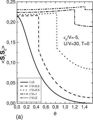
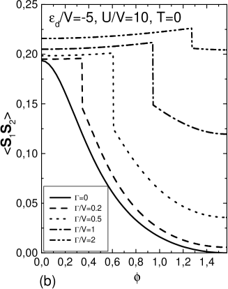
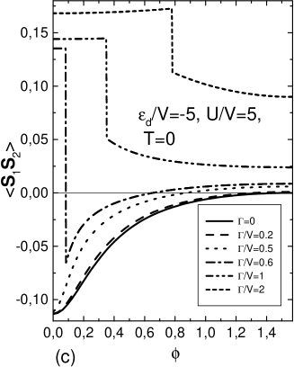
Figure 2: Zero-temperature magnetic correlation $<\mathbf{S}_{1}\mathbf{S}_{2}>$ as a function of $\phi$, for $\varepsilon_{d}/V=-5$ and three different values of $U/V=$ 30 (a), 10 (b), and 5 (c).In (a) and (b)we take $\Gamma/V=$ 0, 0.2, 0.5, 1, and 2. For (c) we use $\Gamma/V=$ 0, 0.2, 0.5, 0.6, and 1

For $\phi=0$, we have the ground state $\alpha_{2\uparrow}^{\dagger}|3,+1/2>_{0}$ and we can write $<\mathbf{S}_{1}\mathbf{S}_{2}>=0.25(b_{1}^{2}+b_{2}^{2})$. When $\Gamma$ is increases, we can see that $|b_{1}|$ increases (see Eq. 11) given more influence of the ferromagnetic state ($|h1>=\alpha_{1\downarrow}^{\dagger}|+>$) for the impurities in the ground state. As a consequence, we can see that the ferromagnetic correlation increases with $\Gamma$ for $\phi=0$ at zero temperature. For $U/|\Delta|\rightarrow\infty$ and $\Gamma=0$, this ferromagnetic correlation reduces to $(1-\Delta/R)/8$. When $\phi$ increases up to $\phi_{c}$ we can observe a ¨jump¨ or discontinuity in $<\mathbf{S}_{1}\mathbf{S}_{2}>$ showing the transition from $S_{z}=+1$ ground state to $S_{z}=0$. For $\phi=\pi/2$, the magnetic correlation take the minimum value. This value, in the Kondo limit of each impurity ($U/|\Delta|\rightarrow\infty$, $V/|\Delta|<<1$), gives $<\mathbf{S}_{1}\mathbf{S}_{2}>=0.25(a_{2}^{2}+\frac{2}{3}a_{3}^{2}-\frac{2}{\sqrt{3}}a_{1}a_{3})$ . For $\Gamma=0$, $a_{2}=a_{3}=0$, and $<\mathbf{S}_{1}\mathbf{S}_{2}>=0$. In (Fig. 2(c)) we show the I.V. regime ($U\leq|\varepsilon_{d}-\varepsilon_{F}|$). For large values of $\Gamma/V$, we have the $S_{z}=+1$ ground state at $\phi=0$ and we can see that $<\mathbf{S}_{1}\mathbf{S}_{2}>$ has the same behavior observed in Fig. 2(a) and (b). For small values of $\Gamma/V$, the $S_{z}=0$ ground state take place and using $|4,0>_{0}$ we can write $<\mathbf{S}_{1}\mathbf{S}_{2}>=\frac{-3}{4}c_{5}^{2}$. So that, we have always antiferromagnetic correlation between the impurities. Finally, for intermediate values of $\Gamma/V$ ($0.6$), we observe the transition from ferromagnetic to antiferromagnetic correlation at $\phi=\phi_{c}$. In Fig. 1(c), for $\Gamma/V=0.6$ and $\phi=0$, we can see that a very small value of $|E_{K}|$ occurs. Due to this fact, the transition can take place only at small values of $\phi_{c}$.

For $\Gamma=0$ (solid lines in Fig. 1and Fig. 2), the antiferromagnetic coupling between itinerant electrons disappears and the model Hamiltonian is spin conserving. Therefore, the first triplet excited state has the lower eigenvalue $\lambda_{S_{z}=1}$ (three times degenerate $S_{z}=\pm 1,0$), and we can see that $E_{K}$ gives the low-energy spin excitation in this model (Kondo energy). This energy decreases continuously from the maximum value at $\phi=\pi/2$, where two independent ($H_{Aj}$) Anderson models take place, to zero for $\phi=0$, with the impurities in the limit of very strong interaction regime, where the states $|3,\pm 1/2>$ play the role of an effective localized spin 1/2 which coupled to the band states $\alpha_{2\sigma}^{\dagger}$ produce the physics that governs the ground state of the Kondo model. Therefore, when the distance between the impurities decreases, the interaction between the impurities via the conduction electrons increases and reduces the $E_{K}$ energy. Furthermore, in according to the Kondo Physics, the magnetic moment at each impurity site $j$ given by: $\mathbf{m}_{j}=\sum_{\sigma,\sigma^{\prime}}<d_{j\sigma}^{\dagger}\mathbf{S}_{\sigma,\sigma^{\prime}}d_{j\sigma^{\prime}}>$, where $\mathbf{S}_{\sigma,\sigma^{\prime}}$ are the standard Pauli matrices, gives always zero for any value of $\phi$. On the contrary, for $\Gamma\neq 0$, the model Hamiltonian is spin non-conserving and we obtain $\mathbf{m}_{j}\neq 0$. We show in Fig. 3, for $|\varepsilon_{d}-\varepsilon_{F}|<U$, the magnitude of the magnetic moment $|\mathbf{m}_{j}|$ as a function of $\phi$.

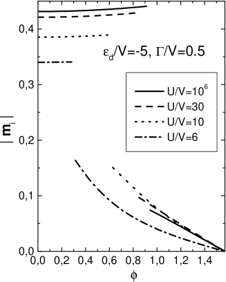
Figure 3: The magnitude of the magnetic moment at each impurity site $|\mathbf{m}_{i}|$ as a function of $\phi$, for $\varepsilon_{d}/V=-5$, $\Gamma/V=0.5$, and four different values of $U/V=10^{6}$, 30, 10, and 6.

The figure shows the region for $\phi<\phi_{c}$, where we observe a very weak dependence on $\phi$ for the corresponding magnetic moment at $\phi=0$, where we can write $|\mathbf{m}_{j}|=0.25*(2b_{1}^{2}+b_{3}^{2}+b_{5}^{2})$. For $\phi_{c}=\phi$, we observe the discontinuity showing the transition from $S_{z}=+1$ ground state to $S_{z}=0$, and finally, for $\phi_{c}<\phi$ we can see that $|\mathbf{m}_{j}|$ decreases and reduces to zero at $\phi=pi/2$ (see $|4,0>_{\pi/2}$). For $U/V=6$, far from the strong Kondo limit, we can observe an important reduction of the magnetic moment.

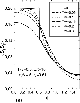
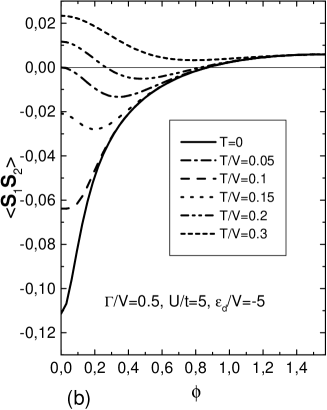
Figure 4: Zero-temperature magnetic correlation $<\mathbf{S}_{1}\mathbf{S}_{2}>$ as a function of $\phi$, for $\varepsilon_{d}/V=-5$, $\Gamma/V=0.5$ , and different values of temperature. In Fig. 4(a) we show the case of $U/V=10$ and Fig. 4(b) shows $U/V=5$

In Fig. 4, we show the magnetic correlations $<\mathbf{S}_{1}\mathbf{S}_{2}>$ as a function of $\phi$, for $\varepsilon_{d}/V=-5$, $\Gamma/V=0.5$, and different values of temperature ($T$). For $U/V=$ $10$, in the Kondo region, Fig. 4(a) shows different behavior depending on the value of $\phi$ related to $\phi_{c}$. For small values ($\phi<\phi_{c}\simeq 0.61$) and very low temperatures, results show very strong ferromagnetic correlation due to de ground state $\alpha_{2\uparrow}^{\dagger}|3,+1/2>_{0}$. Therefore, as the temperature increases, the contribution of the low energy levels reduce the magnetic correlation. On the contrary, for $\phi>\phi_{c}$, it is interesting to note that at low temperatures, thermodynamical excitations to the low excited states give additional contribution to the ferromagnetic correlation. This is an expected result in a Kondo energy level scheme (singlete-triplet structure). Therefore, we consider that $\phi_{c}$ as the lowest limit of $\phi$ below which the breakdown of the Kondo theory occurs. Finally, for $\phi\rightarrow\pi/2$, the splitting of the low energy levels decrease, so that, correlation decreases with increasing temperature.

For $U/V=$ $5$, in the I.V. regime, Fig. 4(b) shows the antiferromagnetic correlation between the impurities. We can see that $<\mathbf{S}_{1}\mathbf{S}_{2}>$ increases when $T$ increases. In Fig. 5, we show the temperature dependence of $<\mathbf{S}_{1}\mathbf{S}_{2}>$ for $U/V=10$, $\varepsilon_{d}/V=-5$, $\Gamma/V=0.5$, and different values of $\phi$, around the $\phi_{c}=0.61$.

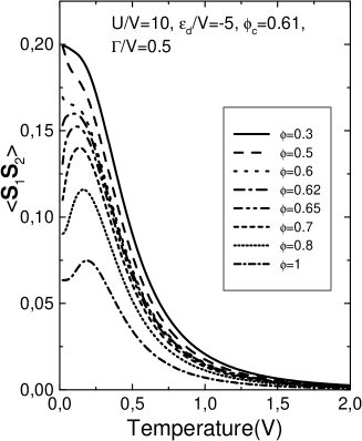
Figure 5: the magnetic correlations $<\mathbf{S}_{1}\mathbf{S}_{2}>$ as a function of temperature, for $\varepsilon_{d}/V=-5$, $U/V=10$, $\Gamma/V=0.5$, and different values of $\phi$ around the $\phi_{c}=0.61$.

At low temperatures, for $\phi\geq\phi_{c}$ the curves show a maximum. This maximum is due to the excitation from the $S_{z}=0$ ground state to the low excited states $S_{z}=+1,0,-1$. When $\phi$ is increases from $\phi_{c}$, the maximum becomes more significant and according to the above discussion in Fig. 4, we consider that the temperature at the maximum gives a rough measure of the Kondo temperature in this model. The curves also show how the maximum moves to low temperatures (the Kondo temperature goes down) when $\phi$ (the distance between impurities) is decreased. For $\phi<\phi_{c}$, the maximum disappears and the Kondo regime is impossible.

IV CONCLUSIONS

We have extended the zero-bandwidth limit of the two-impurity Anderson model to include the effect of an antiferromagnetic gap in the conduction band states. We have studied, as a function of $\phi=\mathbf{k}_{F}\mathbf{\cdot r}$, the lowest excitation energy, the magnetic moment at each impurity site, and the magnetic correlation between the impurities in this model. In the region of parameters where the impurities are in the Kondo regime, as a function of $\phi$, we have shown that a very interesting competition between the AF gap and the Kondo physics of the two impurities take place. At zero temperature, when the impurities are close enough ($\phi<\phi_{c}$), the AF splitting governs the physics of the system and the local moment of the impurities are frozen in a state with very strong ferromagnetic correlation between the impurities, and roughly independent of the distance. On the contrary, when the impurities are sufficiently far apart ($\phi>\phi_{c}$) and the AF gap is not too large, the scenario of Kondo physics takes place: a non-magnetic ground state with the possibility of spin-flip excitation can occurs. Here, the ferromagnetic $<\mathbf{S}_{1}\mathbf{S}_{2}>$ decreases when $\phi$ is increased from $\phi_{c}$, but the complete decoupling of the impurities never occurs. In addition, the presence of the AF gap gives a non-zero magnetic moment $\mathbf{m}_{j}$ at each impurity site, showing a non complete kondo screening of the impurities. Also, we can see that the residual magnetic moment decreases when $\phi$ is increased. Finally, the zero-bandwidth limit approach used here gives a new contribution to understand the very relevant and difficult problem of two magnetic impurities in an antiferromagnetic metal. We expect that new experimental results in nanodevices will confirm some of the theoretical predictions obtained here.

Acknowledgments

The author acknowledges many illuminating discussions with Blas Alascio.This work was supported by the Consejo Nacional de Investigaciones Científicas y Técnicas (CONICET).