Deformed matrix models, supersymmetric lattice twists and ${\cal N}={\textstyle{\frac{1}{4}}}$ supersymmetry

Abstract:

A manifestly supersymmetric nonperturbative matrix regularization for a twisted version of ${\cal N}=(8,8)$ theory on a curved background (a two-sphere) is constructed. Both continuum and the matrix regularization respect four exact scalar supersymmetries under a twisted version of the supersymmetry algebra. We then discuss a succinct ${\cal Q}=1$ deformed matrix model regularization of ${\cal N}=4$ SYM in $d=4$, which is equivalent to a non-commutative $A_{4}^{*}$ orbifold lattice formulation. Motivated by recent progress in supersymmetric lattices, we also propose a ${\cal N}={\textstyle{\frac{1}{4}}}$ supersymmetry preserving deformation of ${\cal N}=4$ SYM theory on $\mathbb{R}^{4}$. In this class of ${\cal N}={\textstyle{\frac{1}{4}}}$ theories, both the regularized and continuum theory respect the same set of (scalar) supersymmetry. By using the equivalence of the deformed matrix models with the lattice formulations, we give a very simple physical argument on why the exact lattice supersymmetry must be a subset of scalar subalgebra. This argument disagrees with the recent claims of the link approach, for which we give a new interpretation.

1 Introduction

This paper has three goals: One is to construct a manifestly supersymmetric matrix (non-lattice) regularization for certain twisted supersymmetric gauge theories formulated on curved backgrounds, such as $S^{2}$ or $S^{2}\times\mathbb{R}$. The other purpose is to discuss the global supersymmetry in the context of twisted supersymmetry, deformed (supersymmetric) matrix models, supersymmetric lattices, and supersymmetry in curved spaces. We hope to provide a sharp meaning to the notion of exact lattice supersymmetry by doing this. Our last goal is to introduce a simpler deformed matrix model regularization for ${\cal N}=4$ supersymmetric Yang-Mills (SYM) theory in $d=4$ dimensions and discuss its relation to the supersymmetric lattice regularization.

It is well-known that global scalar supersymmetry may be carried to curved spaces if a twisted version of the supersymmetry algebra is used [1]. On a flat space, twisting is a procedure which embeds a new Lorentz group into the product of the usual Lorentz and a global symmetry group. Usually, this is done in such a way that some of the spinors of the Lorentz symmetry turns into spin-0 scalars under the new twisted Lorentz group, see for example [2]. The twisted theories can be carried into curved backgrounds while preserving the (nilpotent) scalar supersymmetry generators, or the scalar subalgebra. A subclass of twisted theories which admits scalar supercharge may also be defined on lattices without upsetting the scalar subalgebra. (Not all twisted theories with a nilpotent supercharge admit a lattice regularization, see the discussion in §7.1) We refer to this subclass as supersymmetric lattice twists or SL-twists for short. The existence of a nilpotent scalar supersymmetry $Q^{2}=0$ is sufficient to formulate a topologically twisted version of supersymmetric gauge theories on curved spaces. The same criterion, however, is necessary but not sufficient to construct a physical (non-topological) supersymmetric theory on a lattice.

Motivated by these general observations, we first construct a deformed supersymmetric matrix model regularization for a twisted theory on curved background, a two-sphere $S^{2}$. The remarkable property of this construction is that both the regularized theory and continuum theory respect the same set of scalar supersymmetries. Our target theory is a twisted version (which we refer as A-twist) of ${\cal N}=(8,8)$ SYM theory with gauge group $U(k)$ residing on a two-sphere, $S^{2}$. Both the deformed matrix model and the A-twist has ${\cal Q}=4$ scalar supersymmetries and these are the exact supersymmetries of the target theory on $S^{2}$, with no enhancement of supersymmetry in the continuum limit.

Next, we study a $\beta$ (flux) deformation of the Type IIB matrix model. The continuum limit of this model is ${\cal N}=(8,8)$ SYM theory on flat torus, $T^{2}$. The regularized matrix model has ${\cal Q}=4$ scalar supersymmetries, which are the scalar set of supersymmetries of a B-twist of ${\cal N}=(8,8)$ target theory. In the continuum limit, the supersymmetry enhances to the full sixteen supersymmetries. A more interesting case is a certain two-flux deformation of the matrix model. This deformation preserves only ${\cal Q}=1$ out of ${\cal Q}=16$ supersymmetries, and generates the ${\cal N}=4$ SYM on $T^{4}$ in its classical continuum limit. We will benefit from the relation of the deformed matrix models and supersymmetric lattices in the discussion of the exact global supersymmetries of various lattice formulations.

In recent years, there has been significant progress on the non-perturbative lattice construction for the supersymmetric gauge theories. Various approaches are used to construct supersymmetric lattices with exact supersymmetry at finite lattice spacing. One such approach is the orbifold constructions which preserve a nilpotent subset of supersymmetries [10, 11, 12]. Also see [13, 14, 15, 16, 17, 18] for related work. Catterall [19, 20, 21, 22] and Sugino [23, 24, 25, 26, 27], starting with a “topologically” twisted form of the target theories, successfully preserved a scalar (nilpotent) subset of supersymmetries on the lattice. The relation between these three formulations was not clear at first.

Motivated by the unconventional aspects of supersymmetric orbifold lattices, such as scalars of the target theories residing on the links (rather than on sites) and fermions filling single-valued integer spin representations (rather than being double-valued spinors), Ref.[28] showed that all the supersymmetric orbifold lattices do indeed produce a twisted version of the supersymmetric gauge theories in their continuum. The main point of Ref.[28] is depicted in Fig. 1. This observation, merged the “topological” approach and supersymmetric orbifold lattices at the conceptual level. Soon after, Catterall [29] showed that, the use of the correct twist together with the geometrical discretization rules produce the supersymmetric lattice actions for the orbifold lattices. More recent important work by Takimi [30], and Damgaard et.al. [31, 32, 33] demonstrated the equivalence of these lattice formulations even at finite lattice spacing. Ref.[34] also provided a full classification of the supersymmetric lattices that can be obtained by orbifolding and argued for uniqueness in certain cases.

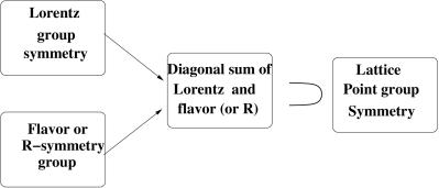
Figure 1: Twisting is one of the the main ideas in the formulation of i) supersymmetric lattices for physical SYM theories, ii) the staggered fermion formulation of lattice QCD, and iii) in the formulation of topological versions of SYM theories on curved spaces. [In literature, twisting is sometimes referred as “topological twisting” due to its applications to topological theories. This is a misnomer.] In neither of the first two cases (which is the main interest of this paper), the lattice point group symmetry may be considered as a sub-group of Lorentz symmetry. It is in fact a subgroup of the diagonal sum of the Lorentz and $G_{\rm global}$, referred as twisted Lorentz group $SO(4)^{\prime}$. $G_{\rm global}$ is an ${\cal R}$-symmetry in the case of supersymmetric theories and is a flavor symmetry in the case of QCD. In both lattice formulations, the fermions are in single-valued, integer spin representation of $SO(4)^{\prime}$ and its discrete subgroups. Of course, by undoing the twist, we recover usual fermions with double-valued spinor representation under $SO(4)$. The figure is adapted from Ref.[35].

There is one other approach to lattice supersymmetry which aims to preserve all the supersymmetries on the lattice, not only the nil-potent scalar supercharges. This approach is also motivated by the twisted form of the supersymmetry algebra and Dirac-Kähler structure of the fermions. It is referred as link approach in D’Adda et.al. [37, 38, 39, 40]. The claim of preserving the whole set of supersymmetries is debated in Ref.[41, 42], with a negative conclusion. On the other hand, the lattice structures on the link approach can be obtained by orbifold projections and in fact, these two approaches are also equivalent as shown in [32]. However, some lattices of link approach constructions, which are claimed to possess all the supersymmetries, can be obtained by orbifold projections which preserve either no supersymmetry, or just few scalar supercharges according to the criteria of [10, 43]. In our opinion, Ref. [32] answered this question satisfactorily by showing that whatever supersymmetry remains intact under the orbifold projection is indeed the exact supersymmetry on the lattice. However, [44, 45] asserted the consistency of the link approach despite Ref.[41, 42, 32]. Here, we will give an independent and simpler argument which shows that the amount of global supersymmetries preserved in lattice regularization of the extended supersymmetric gauge theories is always the subset of scalar supersymmetries, and not the whole set of supersymmetry.

The merit of our argument is in its conceptual simplicity. We will benefit from the (supersymmetric) deformed matrix models. Recall that in $d=4$ dimensions, the $\beta$ [3] or a mass deformation of superpotential reduce the ${\cal N}=4$ SYM down to ${\cal N}=1$. There is no ambiguity in the amount of global supersymmetry here, because the other twelve supersymmetries are explicitly spoiled by the deformation. We will consider similar ${\cal Q}=1$ [6] and ${\cal Q}=4$ supersymmetry preserving deformation of ${\cal Q}=16$ Type IIB model. The equivalence of the deformed supersymmetric matrix model to supersymmetric lattices is explicitly given in [6] and is summarized in §5. The reason that I choose to go through this detour is to avoid the technical discussion of the modified Leibniz rule or its spin-offs such as “link supercharge” altogether. Our argument is very simple. Since the $\beta$-deformed matrix model is equivalent to the lattice regularization, the existence of the full set of supersymmetry in the lattice formulation would have implied that the $\beta$-deformation does not reduce the amount of supersymmetry, which is a contradiction. This argument also leads us to the conclusion that exact lattice supersymmetry must be a subset of the scalar supersymmetry subalgebra.

The question of whether we can preserve the whole set of supersymmetries of a continuum gauge theory in its lattice (or matrix) regularization leads us to a surprising reverse-engineering. There exist deformations of ${\cal N}=4$ SYM theory on $\mathbb{R}^{4}$ or $T^{4}$ which preserve only ${\cal N}={\textstyle{\frac{1}{4}}}$ (or ${\cal Q}=1$) supersymmetry. The idea is to deform the twisted action such that only scalar super-charge remains as a global supersymmetry. Although these theories looks like a BRST-like gauge fixing of an underlying gauge invariant theory, I was unable to construct them this way. A physical interpretation for the ${\cal N}={\textstyle{\frac{1}{4}}}$ theories on flat space is currently lacking, although their non-perturbative lattice and matrix regularizations exist, and are given here. The generalization of these twisted-deformed actions to other dimensions is obvious.

Finally, I discuss twisting in a more general context (outside supersymmetry or topological twisting) in §8 where I rephrase the staggered and reduced staggered fermions of lattice QCD as particularly elegant applications of the twisting idea, see Fig.1. In these cases, the ${\cal R}$-symmetry is replaced by the flavor symmetry of QCD.

2 Target theories: Twisted ${\cal N}=(8,8)$ SYM theories on $S^{2}$ and $T^{2}$

Our two dimensional target theories are the twisted versions of the ${\cal N}=(8,8)$ (or ${\cal Q}=16$) supersymmetric Yang-Mills theory formulated on a two-sphere, $S^{2}$ and on a two-torus $T^{2}$. The ${\cal N}=(8,8)$ theory on $\mathbb{R}^{2}$ can be obtained as the dimensional reduction of the ${\cal N}=1$ gauge theory on $\mathbb{R}^{10}$ down to $\mathbb{R}^{2}$. The ten dimensional theory possess an $SO(10)$ Euclidean Lorentz rotation group. Upon reduction, $SO(10)$ group decompose into

$$SO(10)\longrightarrow\left(\begin{array}[]{c|c}SO(2)&\\ \hline\cr&SO(8)\end{array}\right)$$ (3)

where $SO(2)$ is the two dimensional Lorentz symmetry acting on $\mathbb{R}^{2}$ and $SO(8)_{\cal R}$ is the internal ${\cal R}$-symmetry group.

We will consider a compactification of the ${\cal Q}=16$ SYM theory on two-sphere, $S^{2}$. A straight forward compactification of a supersymmetric theory on a curved manifold breaks all the supersymmetries, since there are no covariantly constant spinors on curved spaces. This can be evaded by using a twisting procedure which turns some of the (spinor) supersymmetries into scalars under a new Lorentz group. The scalar supersymmetries are globally defined even when the underlying manifold is curved. The other supersymmetries of the flat-space theory are no longer symmetries in the global sense on $S^{2}$.

The fermions and supercharges transform under the spin group of $SO(2)\times SO(8)$ as $({\textstyle{\frac{1}{2}}},{\bf 8})\oplus(-{\textstyle{\frac{1}{2}}},{\bf 8^{\prime}})$ and the scalars and gauge bosons transform as $(1,{\bf 8_{v}})$ and $(\pm 1,{\bf 1})$. Below, we wish to examine two twists of the theory that will accommodate four scalar supersymmetries.

2.1 A-twist

The main idea of twisting is to embed a new rotation group into the product of Lorentz and ${\cal R}$-symmetry groups in such a way that a subset of supercharges transform as scalars. In our particular case, we find an embedding of $SO(2)^{\prime}_{E}$ into $SO(2)_{E}\times SO(8)_{\cal R}$. Let us decompose $SO(8)_{\cal R}\rightarrow SO(4)\times SO(4)\sim SU(2)_{A}\times SU(2)_{B}\times SU(2)_{L}\times SU(2)_{R}$. Therefore, under

$$SO(2)_{E}\times[SU(2)]^{4}$$ (4)

the fermions and bosons branch as

$${\rm scalars}:\;\;(0,{\bf 2,2,1,1})\oplus(0,{\bf 1,1,2,2})\qquad{\rm gauge\;bosons}:\;\;(\pm 1,{\bf 1,1,1,1})$$ (5)

(6)

$${\rm fermions:}\;\;({\textstyle{\frac{1}{2}}},{\bf 2,1,2,1})\oplus(-{\textstyle{\frac{1}{2}}},{\bf 2,1,1,2})\oplus({\textstyle{\frac{1}{2}}},{\bf 1,2,2,1})\oplus(-{\textstyle{\frac{1}{2}}},{\bf 1,2,1,2})$$ (7)

One can use, the $U(1)_{A}$ subgroup of the $SU(2)_{A}$ to construct a twisted rotation group

$$U(1)^{\prime}_{E}={\rm Diag}(U(1)_{E}\times U(1)_{A})\qquad.$$ (8)

and declare $U(1)^{\prime}_{E}\sim SO(2)^{\prime}_{E}$ as the new Lorentz group. This is the procedure of twisting. Since the $[SU(2)]^{3}$ subgroup of the full ${\cal R}$-symmetry remains intact, it will be an ${\cal R}$-symmetry group of the twisted version. Under $U(1)^{\prime}_{E}\times[SU(2)]^{3}$, the transformation properties of fields are

$${\rm fermions}\longrightarrow(1,{\bf 1,2,1})\oplus(0,{\bf 1,2,1})\oplus(-1,{\bf 1,1,2})\oplus(0,{\bf 1,1,2})\oplus({\textstyle{\frac{1}{2}}},{\bf 2,2,1})\oplus(-{\textstyle{\frac{1}{2}}},{\bf 2,1,2})\qquad$$ (9)

(10)

$${\rm scalars}\longrightarrow(\pm{\textstyle{\frac{1}{2}}},{\bf 2,1,1})\oplus(0,{\bf 1,2,2})\qquad{\rm gauge\;bosons}\longrightarrow(\pm 1,{\bf 1,1,1})$$ (11)

Four of the fermionic degrees of freedom are neutral under the twisted Lorentz group $U(1)^{\prime}_{E}$, and therefore they transform as scalars. The same argument is also true for the supercharges, and consequently the sixteen supercharges of the original theory decompose precisely as fermions in eq. (11). Four of them are scalars

$${\rm Scalar\;\;supercharges:}(0,{\bf 1,2,1})\oplus(0,{\bf 1,1,2})$$ (12)

and they can be defined globally on curved two-manifolds.

There is a natural supermultiplet structure that can be read-off from the transformation properties of the fields and supercharges:

$$\begin{array}[]{|c|c|c|}\hline\cr&{\rm Bosons}&{\rm Fermions}\cr\hline\cr U(1)^{\prime}_{E}\;\;\;{\rm scalars}:&(0,{\bf 1,2,2})&(0,{\bf 1,2,1})\oplus\;\;(0,{\bf 1,1,2})\cr&&\cr\hline\cr U(1)^{\prime}_{E}\;\;\;{\rm spinors}:&(\pm{\textstyle{\frac{1}{2}}},{\bf 2,1,1}),&\;\;({\textstyle{\frac{1}{2}}},{\bf 2,2,1}),\;\;(-{\textstyle{\frac{1}{2}}},{\bf 2,1,2})\cr&&\cr\hline\cr U(1)^{\prime}_{E}\;\;\;{\rm vectors}:&(\pm 1,{\bf 1,1,1}),&\;\;(1,{\bf 1,2,1}),\;\;(-1,{\bf 1,1,2})\cr&&\cr\hline\cr\end{array}$$ (20)

The supermultiplets transform as their lowest components and are respectively scalars, spinors and vectors under $U(1)^{\prime}_{E}$: Unlike the supersymmetric lattice twists which associate all the degrees of freedom with integer valued representations of the twisted rotation group, this twist has double-valued spinor representations as well.

The A-twist of the gauge theory on $S^{2}$ arises naturally out of a ${\cal Q}=4$ supersymmetry preserving mass deformation of ${\cal Q}=16$ type IIB matrix model, as it will be discussed in §3.4.

2.2 B-twist

The supersymmetric lattice twists have no half-integer representation under the twisted group. We can build such a twist starting with eq. (11) and by taking the diagonal sum of the $U(1)^{\prime}_{E}$ with the $U(1)_{B}$ subgroup of $SU(2)_{B}$:

$$U(1)^{\prime\prime}_{E}={\rm Diag}(U(1)^{\prime}_{E}\times U(1)_{B})={\rm Diag}(U(1)_{E}\times U(1)_{A}\times U(1)_{B})$$ (21)

This amounts to defining a charge $Q_{E}^{\prime\prime}$ as

$$Q^{\prime\prime}_{E}=Q_{E}+Q_{A}+Q_{B}$$ (22)

under $SO(2)_{E}^{\prime\prime}\sim U(1)^{\prime\prime}_{E}$. Under $U(1)^{\prime\prime}_{E}\times SU(2)_{L}\times SU(2)_{R}$, we have

$${\rm scalars}\longrightarrow(\pm 1,{\bf 1,1})\oplus 2(0,{\bf 1,1})\oplus(0,{\bf 2,2})\qquad{\rm gauge\;bosons}\longrightarrow(\pm 1,{\bf 1,1})$$ (23)

(24)

$$\rm fermions\longrightarrow 2\times\left[(1,{\bf 2,1})\oplus(0,{\bf 2,1})\oplus(-1,{\bf 1,2})\oplus(0,{\bf 1,2})\right]$$ (25)

This twist is the one which emerges naturally from the $A_{2}^{*}$ hexagonal lattice construction [28]. In §3.6 we will see that the B-twist also appears in a ${\cal Q}=4$ supersymmetry preserving $\beta$-flux deformation of type IIB matrix model.

3 Matrix regularization of target theories on $S^{2}$ and $T^{2}$

In this section, we present a manifestly supersymmetric deformed matrix model regularization for the twisted version of supersymmetric gauge theory on $S^{2}$ and $T^{2}$. The two types of matrix regularizations have manifest ${\cal Q}=4$ supersymmetries, and in their continuum, correspond to A-twist and B-twist, respectively. On $S^{2}$, there is no enhancement of the supersymmetry in the continuum. For $T^{2}$, as in the supersymmetric lattices, generically a nilpotent scalar subset of supersymmetry is preserved exactly on the regularized theory, and the others emerge accidentally in the continuum.

3.1 The Type IIB matrix model in ${\cal Q}=4$ multiplets

To describe our regularization scheme, it is convenient to express the ${\cal Q}=16$ Type IIB matrix theory in a manifestly ${\cal Q}=4$ supersymmetric formalism. This is most easily done by writing the ${\cal N}=4$ SYM in $d=4$ dimensions using ${\cal N}=1$ superfields followed by dimensional reduction down to $d=0$ dimension. The matrix model action is

$$S = \frac{1}{g^{2}}\operatorname{Tr}\biggl{[}\int d^{2}\theta\;d^{2}\kern 0.6pt\overline{\kern-0.6pt\theta\kern-0.6pt}\kern 0.6pt\;\;\kern 0.6pt\overline{\kern-0.6pt\mathbf{Z}\kern-0.6pt}\kern 0.6pt_{m}e^{2{\bf V}}{\mathbf{Z}}^{m}e^{-2{\bf V}}+\;\frac{1}{4}\int d^{2}\theta\;{\bf W}^{\alpha}{\bf W}_{\alpha}+{\rm a.h.}$$

$$+ \frac{\sqrt{2}}{3!}\epsilon_{mnp}\int d^{2}\theta\,{\mathbf{Z}}^{m}[\mathbf{Z}^{n},\mathbf{Z}^{p}]+{\rm a.h.}\biggr{]}$$

Here, $\mathbf{Z}^{m}$, $\kern 0.6pt\overline{\kern-0.6pt\mathbf{Z}\kern-0.6pt}\kern 0.6pt_{m}$, ${\bf V}$ and ${\bf W}_{\alpha}$ are the dimensional reduction of familiar ${\cal N}=1$ chiral, anti-chiral vector and field-strength supermultiplets on $\mathbb{R}^{4}$ down to $d=0$ dimension.

The type IIB matrix model possesses a global $SO(10)$ symmetry and sixteen supersymmetries. The ${\cal Q}=4$ superfield language only makes the

$$SU(3)\times SU(2)\times SU(2)\times U(1)$$ (27)

subgroup manifest. The ${\bf 10}$ bosons and ${\bf 16}$ fermions of $SO(10)$ decompose under eq. (27) as

$${\bf 10}\ \longrightarrow\ z^{m}\oplus\kern 0.6pt\overline{\kern-0.6ptz\kern-0.6pt}\kern 0.6pt_{m}\oplus\tilde{v}\sim({\bf 3,1,1})_{\frac{2}{3}}\oplus({\bf\kern 0.6pt\overline{\kern-0.6pt3\kern-0.6pt}\kern 0.6pt,1,1})_{-\frac{2}{3}}\oplus({\bf 1,2,2})_{0}\ .$$ (28)

$${\bf 16}\ \longrightarrow\ \psi^{m}\oplus\kern 0.6pt\overline{\kern-0.6pt\psi\kern-0.6pt}\kern 0.6pt_{m}\oplus\lambda\oplus\kern 0.6pt\overline{\kern-0.6pt\lambda\kern-0.6pt}\kern 0.6pt\sim({\bf 3,2,1})_{-\frac{1}{{3}}}\oplus({\bf\kern 0.6pt\overline{\kern-0.6pt3\kern-0.6pt}\kern 0.6pt,1,2})_{\frac{1}{{3}}}\oplus({\bf 1,2,1})_{{1}}\oplus({\bf 1,1,2})_{-{1}}\ \$$ (29)

Next, we construct a ${\cal Q}=4$ supersymmetry preserving mass deformation of the matrix model eq. (3.1). The deformed matrix model, around a particular background solution, produces a higher dimensional twisted supersymmetric gauge field theory.

3.2 Mass deformed matrix model and symmetries

The ${\cal Q}=4$ supersymmetry preserving (equal) mass deformation of the ${\cal Q}=16$ supercharge theory is the dimensional reduction of the ${\cal N}=1^{*}$ SYM from $d=4$ down to $d=0$ dimension. The ${\cal N}=1^{*}$ deformation of the ${\cal N}=4$ was studied in Ref. [46]. The deformed “superpotential” is

$$W({\mathbf{Z}}^{m})=\frac{\sqrt{2}}{3!}\epsilon_{mnp}\,{\mathbf{Z}}^{m}[\;\mathbf{Z}^{n},\mathbf{Z}^{p}\;]+\frac{1}{\sqrt{2}}\;m\sum_{p=1}^{3}\;\;(\mathbf{Z}_{p})^{2}$$ (30)

or equivalently, the deformed action is

$$S^{\rm deformed}=S+\frac{1}{\sqrt{2}}m\int d^{2}\theta\;\sum_{p=1}^{3}\;(\mathbf{Z}_{p})^{2}+{\rm a.h.}$$ (31)

The mass deformation preserves the $SO(3)\cong SU(2)$ subgroup of $SU(3)\times U(1)$ ${\cal R}$-symmetry. Since the mass parameter is dimensionful, the $U(1)$ symmetry is explicitly broken. The three dimensional representations of $SU(3)$ split as ${\bf 3}({\bf\kern 0.6pt\overline{\kern-0.6pt3\kern-0.6pt}\kern 0.6pt})\rightarrow{\bf 2}\oplus{\bf 1}$ under $SU(2)$. The $SO(4)\simeq SU(2)\times SU(2)$ ${\cal R}$-symmetry, just like ${\cal Q}=4$ supersymmetry, is not harmed. This means, the mass deformed matrix model has a manifest $[SU(2)]^{3}$ symmetry. The ten bosons and sixteen fermions of the matrix model, under $[SU(2)]^{3}$ symmetry decompose as

$${\bf 10}\ \longrightarrow 2({\bf 2,1,1})\oplus 2({\bf 1,1,1})\oplus({\bf 1,2,2}).$$ (32)

$${\bf 16}\ \longrightarrow({\bf 2,2,1})\oplus({\bf 1,2,1})\oplus({\bf 2,1,2})\oplus({\bf 1,1,2})\oplus({\bf 1,2,1})\oplus({\bf 1,1,2})\ \$$ (33)

As we have seen in §2, the $[SU(2)]^{3}$ symmetry is the ${\cal R}$-symmetry group of the A-twist shown in eq. (11). The $U(1)^{\prime}_{E}$ twisted rotation symmetry is not a symmetry of the matrix model. It emerges in the continuum in the same way as the Lorentz symmetry emerges in the continuum limit of a lattice gauge theory.

3.3 Noncommutative moduli space

The zero action configurations of the deformed matrix theory, also called the noncommutative moduli space, is the locus of the bosonic action:

$$S_{bosonic}|_{\cal M}=0$$ (34)

This implies the vanishing of $F$ and $d$ terms and all other bosonic positive definite terms in the action:

$$F_{m}=\frac{\partial W(z^{m})}{\partial z^{m}}=0,\qquad d=-i\sum_{m=1}^{3}[\kern 0.6pt\overline{\kern-0.6ptz\kern-0.6pt}\kern 0.6pt_{m},z^{m}]=0,\qquad[v_{\mu},v_{\nu}]=0,\qquad[v_{\mu},z^{m}]=0\qquad$$ (35)

where $m=1,\ldots 3$ and $\mu=1,\ldots 4$. The $F$-term conditions are

$$[z^{m},z^{n}]=-m\epsilon_{mnp}z^{p}$$ (36)

The anti-hermitian ${\Im}(z^{m})$ satisfies the commutation relations of the $SU(2)$ algebra. Since the $F$-term conditions are not homogeneous under $z\rightarrow cz$ where $c\in\mathbb{C}$, the mass deformed theory (in the chiral multiplet sector) does not possess a moduli space, rather it has a discrete isolated set of classical minima. The solutions of the $F$-terms also satisfy the $d$-term condition. The other conditions in eq. (35) put certain restrictions on the form of $v_{\mu}$, but not $z_{m}$.

The eq. (36) has both reducible and irreducible set of solutions [46]. For example, an irreducible embedding of $SU(2)$ algebra into $U(N)$ yield a target theory with $U(1)$ gauge group. In order to construct the continuum $U(k)$ gauge theory on $S^{2}$, it is more convenient to start with a $U(Nk)$ matrix model and expand the fluctuation around the rank-$N$ background solution of eq. (36). Formally, we have

$$U(Nk)\longrightarrow\underbrace{U(N)}_{S^{2}\;\rm background}\otimes\underbrace{U(k)}_{\rm fluctuations}$$ (37)

The background solution for eq. (36) can explicitly be written as

$$z^{p}=imJ^{p},\qquad{\rm where}\;\;\;[J^{m},J^{n}]=i\epsilon_{mnp}J^{p}$$ (38)

where $J_{p}$ are generators of $SU(2)$ algebra. The irreducible embedding of $SU(2)$ into $U(N)$ is an angular momentum

$$j\equiv\frac{N-1}{2}$$ (39)

representation. The eigenvalues of each ${\Im}(z^{p})$ ranges in the interval $m\left[-\frac{N-1}{2},\ldots,\frac{N-1}{2}\right]$. However, these matrices do not commute with each other, and consequently, the moduli space is noncommutative. The eigenvalues lies on the surface of a sphere (which is often referred as “a fuzzy sphere”) in moduli space:

$$\sum_{p=1}^{3}\;(z^{p})^{2}=m^{2}\sum_{p=1}^{3}\;(J^{p})^{2}=m^{2}\;j(j+1)\;1_{N}=\frac{m^{2}(N^{2}-1)}{4}1_{N}$$ (40)

where the last equality follows from eq. (39). The radius of this fuzzy sphere $R_{\rm fuzzy}$ in the moduli space is the UV cut-off ($\Lambda_{\rm UV}$) of the matrix regularization

$$R_{\rm fuzzy}=\frac{mN}{2}=\Lambda_{\rm UV},$$ (41)

up to lower order terms in $1/N$. In the continuum limit, the size of this fuzzy sphere diverges in an analogous manner with the Brillouin zone of a lattice gauge theory, whereas the base space of our target theory has a fixed size determined by $m^{-1}$ , the IR scale.

In what follows, the non-commuting zero action configurations $J^{p},\;p=1,2,3$ play two roles. They generate the $S^{2}$ background and the “hopping” (kinetic) terms in the target $U(k)$ theory.

3.4 Classical spectrum and “onion ring” Brillouin zone

In order to analyze the quadratic fluctuations of the action, we expand the superfields around the zero action configuration:

$$\mathbf{Z}_{p}=\langle\mathbf{Z}_{p}\rangle+\widetilde{\mathbf{Z}}_{p}=im\;J_{p}\otimes{\bf 1}_{k}+\widetilde{\mathbf{Z}}_{p}$$ (42)

where $\widetilde{\mathbf{Z}}_{p}$ denotes the fluctuations. We expand generic matrix field ${\bf X}$ in our action as

$${\bf X}=\sum_{l,m}Y_{lm}\otimes{\bf X}_{lm}$$ (43)

where $Y_{lm}$ are $N\times N$ matrices (given below), associated with the angular momentum mode $l,m$. The fields ${\bf X}_{lm}$ is the $U(k)$ algebra valued field associated with the momentum $l,m$ in a spherical decomposition.

In eq. (42), the fluctuation matrix $\widetilde{\mathbf{Z}}$ is a $GL(Nk,\mathbb{C})$ valued matrix. The zero action configuration matrices can be used to form a complete orthonormal matrix basis for $GL(N,\mathbb{C})$. Since $GL(N,\mathbb{C})$ is $N^{2}$ complex dimensional vector space, we need $N^{2}$ basis matrices. A complete orthonormal basis is generated by using the three $J_{p}$ matrices, and by just mimicking the spherical harmonics, $Y_{lm}$. For example, for $GL(3,\mathbb{C})$, a complete orthogonal basis ${\cal B}(S^{2})$ composed of nine three by three matrices are given by

$${\cal B}(S^{2})\equiv\Big{\{}1,J_{z},J_{\pm},J_{\pm}^{2},J_{z}J_{\pm},(3J_{z}^{2}-1)\Big{\}}\sim\Big{\{}Y_{00},Y_{10},Y_{1,\pm 1},Y_{2,\pm 2},Y_{2,\pm 1},Y_{2,0}\Big{\}}$$ (44)

The classical spectrum of the fermions and bosons can be found by studying the fluctuations around the background. This is a straightforward calculation along the lines of analysis of [47] and [6]. In particular, the details of the classical analysis are literally identical to the deconstruction of the Maldacena-Núñez compactification on $\mathbb{R}^{4}\times S^{2}$, starting with ${\cal N}=1^{*}$ SYM theory in $d=4$ dimensions, and are discussed thoroughly in [47]. Hence, this classical analysis will not be repeated here. The interaction terms as well work precisely as in [6] and [47]. This means, at the classical level, our deformed matrix model produces the target theory on $S^{2}$ correctly. Below, we discuss some interesting physical aspects of the matrix regularizations.

The spectrum of Grassmann even and odd modes of the matrix model, their level degeneracy and their transformation properties under the twisted rotation group are given by

$$\begin{array}[]{|c|c|c|c|}\hline\cr{\rm Free\;Spectrum}&{\rm Grassmann\;odd}&{\rm Grassmann\;even}&SO(2)_{E}^{\prime}\cr&&&\cr\hline\cr M^{2}_{l,m}=m^{2}\;l(l+1),\,\,\,l=0,1,2,\ldots&4(2l+1),&4(2l+1)&{\rm scalar}\cr&&&\cr\hline\cr M^{2}_{l^{\prime},m^{\prime}}=m^{2}\;(l^{\prime}+{\textstyle{\frac{1}{2}}})^{2},\,\,\,l^{\prime}={\textstyle{\frac{1}{2}}},{\textstyle\frac{3}{2}},{\textstyle\frac{5}{2}},\ldots,&8(2l^{\prime}+1)&4(2l^{\prime}+1)&{\rm spinor}\cr&&&\cr\hline\cr M^{2}_{l,m}=m^{2}\;l(l+1),\,\,\,l=1,2,3,\ldots,&4(2l+1)&2(2l+1)&{\rm vector}\cr&&&\cr\hline\cr\end{array}.$$ (53)

The three types of the spectrum can be naturally associated with the truncated spectrum of spin-0, spin-${\textstyle{\frac{1}{2}}}$ and spin-$1$ fields on $S^{2}$. The spectral degeneracy of the Grassmann even and odd spin-0, spin-${\textstyle{\frac{1}{2}}}$ and spin-$1$ modes is a consequence of the exact supersymmetry of the deformed matrix model.

Brillouin zone: The spectrum shown in eq. (53) also provides a notion of the Brillouin zone for the matrix regularization. In the penultimate line of eq. (53), define $l=(l^{\prime}+{\textstyle{\frac{1}{2}}}),\;l=1,2,3\ldots$. The Brillouin zone is composed of circular shells, like the onion rings and $l^{th}$ shell accommodates $(2l+1)$ states. The cut-off is determined by the size of the matrices in the matrix regularization, $N$, and $j_{max}=\frac{N-1}{2}$ and the UV cut-off is $\Lambda_{\rm UV}=m\frac{N}{2}$. As in the lattice regularization, wavelengths below the length scale $\Lambda^{-1}_{\rm UV}$ are not present in the matrix regularized theory. In the continuum limit, we take the cut-off $\Lambda_{\rm UV}$ to infinity while keeping $m$ fixed (the inverse size of the two-sphere) and taking $N\rightarrow\infty$. In the moduli space, this corresponds to taking radius of the fuzzy sphere to infinity, similar to the deconstruction and supersymmetric lattices where the continuum limit is a trajectory out to infinity in the moduli space.

3.5 A-twist and mass deformation

Fermions: Clearly, the spectrum of the Grassmann odd variables shown in eq. (53) is not what one would naively expect from the eigenvalue spectrum of a Dirac operator on a two-sphere $S^{2}$. Instead, it is a mix of truncated spectrum of spin-0, spin-${\textstyle{\frac{1}{2}}}$ and spin-$1$ fields on a sphere. In eq. (53), another bizarre feature at first glance is the appearance of fermion zero modes. However, it is well known that, the eigenvalue spectrum of the Dirac operator on $S^{2}$, (and in general in any positively curved background) has a gap due to spin connection.

Of course, although the fermionic spectrum sounds incorrect for a naive (no supersymmetry preserving) compactification of the ${\cal N}=(8,8)$ theory on $S^{2}$, it is on the other hand precisely what one expects from the compactification of the twisted formulation discussed in §2.1. Due to twisting, we have global supersymmetry on $S^{2}$, the spectrum of fermions has four fermionic zero modes, which is in exact correspondences with the presence of four exact supersymmetries of the matrix model eq. (31).

Bosons: The spectrum of bosons coincides with the truncation of the A-twist eq. (11) of the supersymmetric theory, but not with the naive untwisted compactification. Of course, this is consistently tied with what we have presented for fermions in terms of twisting.

3.6 B-twist and $\beta$-flux deformation and target theory on $T^{2}$

The $\beta$-flux deformation of the superpotential is a one-parameter family of deformation given by

$$W({\mathbf{Z}}^{m})_{\beta} =\sqrt{2}{\mathbf{Z}}^{1}(e^{-i\beta/2}\mathbf{Z}^{2}\mathbf{Z}^{3}-e^{+i\beta/2}\mathbf{Z}^{3}\mathbf{Z}^{2})$$ (54)

or equivalently,

$$W({\mathbf{Z}}^{m})_{\beta}=\frac{\sqrt{2}}{3!}\epsilon_{mnp}\,{\mathbf{Z}}^{m}(\;e^{-i\Phi_{np}/2}\mathbf{Z}^{n}\mathbf{Z}^{p}\;-e^{+i\Phi_{np}/2}\mathbf{Z}^{p}\mathbf{Z}^{n}\;)$$ (55)

with obvious identifications. The deformation is respectful to $SU(2)_{L}\times SU(2)_{R}$ ${\cal R}$-symmetry of the matrix model, whereas it only preserves $U(1)^{3}$ subgroup of the $SU(3)\times U(1)$ symmetry. Recall from §2.2 that the $SU(2)_{L}\times SU(2)_{R}$ is also the non-abelian global ${\cal R}$-symmetry of the B-twist .

The $\beta$ flux-deformation does not introduce a dimensionful parameter, unlike the case with mass deformation. However, the $\beta$-flux deformed theory possesses a degenerate manifold of the ground states, a moduli space, where the distance from the origin of the moduli space has an interpretation as an UV cut-off, similar to the supersymmetric orbifold lattices.

The zero action configuration of the $\beta$-flux deformed theory is the solution of eq. (35). Given the superpotential eq. (54), the $F$-term constraints reduce to a slight generalization of the ’t Hooft algebra

$$z^{1}z^{2}=e^{i\beta}z^{2}z^{1},\qquad z^{2}z^{3}=e^{i\beta}z^{3}z^{2},\qquad z^{3}z^{1}=e^{i\beta}z^{1}z^{3}$$ (56)

Let us consider a $U(Nk)$ deformed matrix theory. Our goal is, similar to the mass deformed matrix model, to generate a base space and gauge theory residing on it:

$$U(Nk)\longrightarrow\underbrace{U(N)}_{T^{2}\;\rm background}\otimes\underbrace{U(k)}_{\rm gauge\;fluctuations}$$ (57)

Such constructions at the classical level are standard, for example, for the classical relation between non-supersymmetric TEK model regularization to the non-commutative Yang-Mills theory, see the Refs.[49, 50, 5] and references therein. The non-commutative Yang-Mills theory also possess the commutative limit for appropriate choice of deformation parameters. The construction of the square lattices on $T^{2}$ in matrix regularization is well-known. Below, we additionally point out how to construct the hexagonal $A_{2}^{*}$ lattice without getting into details. Of course, the main point of this section is that $\beta$-flux deformation produce the B-twist in its continuum limit.

Let us choose the deformation matrix as

$$\Phi_{np}=\left[\begin{array}[]{cc|c}&+\frac{2\pi}{N}&-\frac{2\pi}{N}\\ -\frac{2\pi}{N}&&+\frac{2\pi}{N}\\ \hline\cr+\frac{2\pi}{N}&-\frac{2\pi}{N}&\end{array}\right]_{np}$$ (61)

The solutions of the ’t Hooft algebra is given in terms of clock and shift matrices:

$$(P)_{kl}=e^{i2\pi k/N}\delta_{kl},\qquad(Q)_{kl}=\delta_{k+1,l},\qquad k,l=1,\ldots N$$ (62)

We background matrices are

$$\langle z^{1}\rangle=c^{1}P\otimes 1_{k},\qquad\langle z^{2}\rangle=c^{2}Q\otimes 1_{k}\qquad\langle z^{3}\rangle=c^{3}(PQ)^{-1}\otimes 1_{k}$$ (63)

where $c^{i}\in\mathbb{C}$ are complex modulus parameters which are essential in establishing a continuum limit. The presence of these moduli fields is expected. If eq. (56) has a solution, due to its homogeneity under $z^{m}\rightarrow\alpha z^{m}$, it has a continuum of solutions (unlike the mass deformed theory eq. (30)). The conditions $[v_{\mu},z^{m}]=0$ restrict $v_{\mu}$ to a matrix proportional to identity. Since $v_{\mu}$ matrices commute with both $P$ and $Q$, they must be proportional to the Casimir of the ’t Hooft algebra, which is identity. With this configuration of the matrices, the $d$-term constraint and $[v_{\mu},v_{\nu}]=0$ are automatically satisfied. Consequently, classical moduli space is (for $k=1$)

$${\cal M}={\mathbb{R}}^{4}\times{\mathbb{C}}^{3}$$ (64)

The existence of ${\mathbb{C}}^{3}$ along which one can move to infinity is sufficient to produce a continuum ${\cal N}=(8,8)$ theory.

We can map the matrix model to two types of lattices. The analog of the basis for $S^{2}$ eq. (44) can now be constructed by using the clock and shift matrices. The basis matrices are $J_{(p_{1},p_{2})}\sim Q^{p_{1}}P^{p_{2}},\;p_{i}=1,\ldots N$ , where $p_{i}$ gains interpretation as momentum in a two dimensional Brillouin zone. In particular, expressing the fluctuations of the matrix fields as $\widetilde{\mathbf{Z}}=\sum_{{\bf p}}J_{\bf p}\otimes\widetilde{\mathbf{Z}}_{\bf p}$ produces the ${\cal Q}=4$ supersymmetry preserving non-commutative lattice regularization for the ${\cal N}=(8,8)$ target theory. As usual, the square and $A_{2}^{*}$ lattices emerges by expanding around the following points in the moduli space

$${\rm Square\;\;lattice:}\;\;c_{1}=c_{2}=\frac{1}{a},\;\;c_{3}=0,$$ (65)

$${\rm Hexagonal}\;A_{2}^{*}\;\;{\rm lattice}:\;c_{m}=\frac{1}{a},\qquad m=1,2,3$$ (66)

The details of this type of calculations can be found in [6].

3.7 Comments

There are a few points that we wish to emphasize in this construction:

1) The matrix regularization given in eq. (54) has only ${\cal Q}=4$ exact supersymmetries. These are the scalar supersymmetries of the B-twist version of the target theory. Since the target theory is defined on a flat $T^{2}$ (or $\mathbb{R}^{2}$ in its infinite volume limit), the other 12 (non-scalar) supersymmetries arises accidentally in the continuum. Note that as it is in $d=4$ dimensional $\beta$-deformation (the Leigh-Strassler deformation [3]), the remaining twelve supersymmetries are explicitly broken, and are not symmetries of the matrix model in any sense.

2) In matrix model approach, there is no orbifold projection. The $N^{2}k^{2}$ total number of microscopic degrees of freedom of the $U(Nk)$ matrix model transmutes into a non-commutative $U(k)$ lattice gauge theory with $N^{2}$ sites. In the orbifold projection, in order to generate a two dimensional regular lattice, one starts with $U(N^{2}k)$ matrix model, which has $N^{4}k^{2}$ degrees of freedom and projects out by a $(Z_{N})^{2}$ discrete symmetry:

$$U(N^{2}k)\underbrace{\longrightarrow}_{\rm orbifolding}[U(k)]^{N^{2}}$$ (67)

In the matrix regularization, one keeps all the degrees of freedom of the matrix model and in the latter, one removes most degrees of freedom by projections. Orbifolding results in an ordinary SYM theory on a commutative (regular) lattice with nearest neighbor interactions. The matrix regularization has both commutative and non-commutative continuum limits.

3) The $\beta$-deformation of the $d=0$ matrix model can only produce the target theories in even dimensions, $d=2,4$. In orbifold constructions, there is no distinction between even and odd dimensional target theories.

4) It should be noted that our analysis of the fluctuations on both ($S^{2}$ and $T^{2}$) backgrounds is classical. As explained, the mass deformed action has many discrete, isolated minima corresponding to different background configuration of the matrix degrees of freedom and the $\beta$ deformed theory has a classical moduli space. As we have argued, not all these background zero action configurations lead to a regularized field theory on $S^{2}$ and $T^{2}$. In our classical analysis, we choose to expand around a particular minima eq. (42). It is in principle possible that the statistical fluctuations can take the equilibrium state we expand around to another one which does not have “an emergent space” interpretation and hence spoil the whole picture.

Indeed, Refs. [50, 49] recently showed a non-perturbative instability in related bosonic matrix models. The TEK model, which produces the $d=4$ dimensional non-commutative YM theory in its classical continuum limit, fails to be stable non-perturbatively. Ref. [49] also shows that in supersymmetric matrix models, the non-commutative background is stable (even if supersymmetry is broken softly). In this sense, the manifestly supersymmetric matrix model regularizations of the supersymmetric theories should be producing a stable background. According to the criteria of Ref. [49], both of our supersymmetric target theories as well as the supersymmetric deformed matrix models of Refs. [4, 5, 6] are safe. For the detailed discussion, we refer the reader to Ref.[49].

4 A new class of supersymmetric gauge theories: ${\cal N}={\textstyle{\frac{1}{4}}}$ SYM

In this section, motivated by the recent advances in supersymmetric lattice constructions and using ideas from the topological field theories, we define a new class of supersymmetric theories with ${\cal N}={\textstyle{\frac{1}{4}}}$ supersymmetry on $\mathbb{R}^{4}$. This construction will be used to address certain questions about exact lattice supersymmetry, although it may have a wider class of applications.

The approach described in what follows can be applied to extended supersymmetric gauge theories in various dimensions. We will describe it in $d=4$ dimensions, starting with ${\cal N}=4$ SYM theory.

The proposal is as follows: First, we twist the ${\cal N}=4$ SYM theory formulated on $M=\mathbb{R}^{4}$. Then, we deform the action on $\mathbb{R}^{4}$ such that only one out of sixteen supersymmetries is preserved exactly.

Recall that the twisted theories on flat space-times such as $M=\mathbb{R}^{4},\;T^{4}$ are simply a rewriting of the original theories in terms of representation of the new Lorentz group. The twisted theory on $\mathbb{R}^{4}$ preserves the same set of supersymmetries as in the original theory, and the twist can be undone. A well-known way to preserve only the scalar sub-set of supersymmetry is to carry the theory into curved space. This is in essence same as declaring the scalar supersymmetry as some type of BRST operator. Here, we will not do so. Instead, we will simply deform the twisted action on $\mathbb{R}^{4}$ in such a way that only ${\cal N}={\textstyle{\frac{1}{4}}}$ is respected.

4.1 Twist the algebra, deform the action: From ${\cal N}=4$ to ${\cal N}={\textstyle{\frac{1}{4}}}$ on $\mathbb{R}^{4}$

Twisting
The ${\cal N}=4$ theory on $\mathbb{R}^{4}$ can be obtained as the dimensional reduction of the ${\cal N}=1$ gauge theory on $\mathbb{R}^{10}$ down to $\mathbb{R}^{4}$. The ten dimensional theory possess an $SO(10)$ Euclidean Lorentz rotation group. Upon reduction, the $SO(10)$ group decomposes into

$$SO(10)\longrightarrow\left(\begin{array}[]{c|c}SO(4)&\\ \hline\cr&SO(6)\end{array}\right)$$ (70)

where $SO(4)\sim SU(2)_{L}\times SU(2)_{R}$ is the four dimensional Lorentz symmetry action on $\mathbb{R}^{4}$ and $SO(6)_{\cal R}\sim SU(4)_{\cal R}$ is the internal ${\cal R}$-symmetry group.

The ${\bf 16}$ dimensional positive chirality spinor of $SO(10)$ and the sixteen supercharges decompose as

$$Q_{\alpha,I}\oplus\kern 0.6pt\overline{\kern-0.6ptQ\kern-0.6pt}\kern 0.6pt_{\dot{\alpha},I}\sim({\bf 2,1,4})\oplus({\bf 1,2,\bar{4}})\in SU(2)_{L}\times SU(2)_{R}\times SU(4)_{\cal R}$$ (71)

The twisting procedure is a choice of an $[SU(2)\times SU(2)]^{\prime}$ embedding into $SU(2)\times SU(2)\times SU(4)_{\cal R}$. There are three inequivalent twists of ${\cal N}=4$ SYM [46], only one of which emerges naturally from supersymmetric lattices, and the two others do not. The reasons is discussed in detail in §7.1.

The twist which arises naturally in supersymmetric lattices maps all the supercharges (and fermions) into integer spin representation. This correspond to the Dirac-Kähler decomposition of multiple-spinors as often used in lattice gauge theory. This twist arises naturally on $A_{4}^{*}$ or hyper-cubic lattice definition of the ${\cal N}=4$ SYM theory. In order to distinguish the twists which admit a lattice implementation [51] and the ones which do not [46], it seems convenient to address the first class as supersymmetric lattice twists (SL-twists).

In what follows, let us choose an SL-twist. It is most easily described by the decomposition of ${\bf 4}$ of $SU(4)_{\cal R}$ into $({\bf 2,1})\oplus({\bf 1,2})$ and by the diagonal embedding of the twisted Lorentz group,

$$[SU(2)\times SU(2)]^{\prime}\subset{\rm Diag}\Big{(}[SU(2)\times SU(2)]_{\rm Lorentz}\times[SU(2)\times SU(2)]_{\cal R}\Big{)}\;.$$ (72)

The spinors (and supercharges) decompose into $p$-form integer spins:

$$Q_{\alpha,I}\oplus\kern 0.6pt\overline{\kern-0.6ptQ\kern-0.6pt}\kern 0.6pt_{\dot{\alpha},I}\longrightarrow Q^{(0)}\oplus Q^{(1)}\oplus Q^{(2)}\oplus Q^{(3)}\oplus Q^{(4)}$$ (73)

The twisted supersymmetry algebra in four dimensions has one or two nilpotent scalar subalgeras, a particularly useful one being

$$(Q^{(0)})^{2}\equiv Q^{2}=0$$ (74)

which does not care about the background spacetime, and is a charge (which is defined globally) even if the background space is curved or discrete. The higher form supersymmetries, $Q^{(1)}$ for example, cannot be globally defined on a curved space, because of the absence of the covariantly constant four vectors on four manifolds. $Q^{(1)}$ cannot be globally defined on a lattice either, since the anti-commutator $\{\eta Q,\eta_{\mu}Q^{{\mu}}\}\;\cdot\sim\eta\eta_{\mu}P^{\mu}\;\cdot$ is an infinitesimal translation, and there are no infinitesimal translation on the lattice. This tells us that the exact global supersymmetry that can be achieved on lattice and on curved spaces are necessarily the scalar subalgebra.

We label the fermionic matter content of the twisted theory as $p$-form Grassmann variables $(\lambda,\psi^{\mu},\xi_{\mu\nu},\xi^{\mu\nu\rho},\psi_{\mu\nu\rho\sigma})$. The bosonic content is $(z^{\mu},\kern 0.6pt\overline{\kern-0.6ptz\kern-0.6pt}\kern 0.6pt_{\mu},z_{\mu\nu\rho\sigma}\kern 0.6pt\overline{\kern-0.6ptz\kern-0.6pt}\kern 0.6pt^{\mu\nu\rho\sigma})$ where $z^{\mu}=(S^{\mu}+iV^{\mu})/\sqrt{2}$ is a complexified gauge field which is the linear combination of the gauge boson and four scalars of the original theory. The other scalars are the fully anti-symmetric $z_{\mu\nu\rho\sigma}$ and its conjugate. We also need complex gauge covariant derivative ${\cal D}^{\mu}\,\cdot=\partial^{\mu}\cdot+\sqrt{2}[z^{\mu},\,\cdot\,],$ and associated two-form field strength ${\cal F}^{\mu\nu}=-i[{\cal D}^{\mu},{\cal D}^{\nu}]$.

The (off-shell) action of the 0-form supercharge $Q$ is

$$Q\lambda=-id,\qquad Qd=0$$ (75)

$$Qz^{\mu}=\sqrt{2}\,\,\psi^{\mu},\qquad Q\psi^{\mu}=0$$ (76)

$$Q\kern 0.6pt\overline{\kern-0.6ptz\kern-0.6pt}\kern 0.6pt_{\mu}=0$$ (77)

$$Q\xi_{\mu\nu}=-i\kern 0.6pt\overline{\kern-0.6pt{\cal F}\kern-0.6pt}\kern 0.6pt_{\mu\nu}$$ (78)

$$Q\xi^{\nu\rho\sigma}=\sqrt{2}\,{\kern 0.6pt\overline{\kern-0.6pt{\cal D}\kern-0.6pt}\kern 0.6pt}_{\mu}\kern 0.6pt\overline{\kern-0.6ptz\kern-0.6pt}\kern 0.6pt^{\mu\nu\rho\sigma}$$ (79)

$$Qz_{\mu\nu\rho\sigma}=\sqrt{2}\psi_{\mu\nu\rho\sigma},\qquad Q\psi_{\mu\nu\rho\sigma}=0$$ (80)

$$Q\kern 0.6pt\overline{\kern-0.6ptz\kern-0.6pt}\kern 0.6pt^{\mu\nu\rho\sigma}=0$$ (81)

where $d$ is an auxiliary field introduced for the off-shell completion of the scalar supersymmetry subalgebra.

Deform
The ${\cal N}=4$ SYM lagrangian on $\mathbb{R}^{4}$ can be expressed in a way to make only ${\cal N}={\textstyle{\frac{1}{4}}}$ manifest. Obviously, with the spinor supercharges, the minimal amount of supersymmetry that we can have in a supersymmetric theory is ${\cal N}=1$. This constraint can be circumvented upon having a spin-0 scalar supercharge.

The twisted Lagrangian on $\mathbb{R}^{4}$ may be written as a sum of $Q$-exact and $Q$-closed terms:

$${\cal L}= {\cal L}_{exact}+{\cal L}_{closed}={\cal L}_{1}+{\cal L}_{2}+{\cal L}_{3}=Q{\widetilde{\cal L}_{exact}}+{\cal L}_{closed},$$ (82)

where $\widetilde{\cal L}_{exact}={\widetilde{\cal L}}_{e,1}+{\widetilde{\cal L}}_{e,2}$ is given by

$${\widetilde{\cal L}}_{e,1}=\frac{1}{g^{2}}\operatorname{Tr}\Big{(}\lambda({\textstyle{\frac{1}{2}}}id+{\textstyle{\frac{1}{2}}}[\kern 0.6pt\overline{\kern-0.6pt\cal D\kern-0.6pt}\kern 0.6pt_{\mu},{\cal D}^{\mu}]+\textstyle{\frac{1}{24}}[\kern 0.6pt\overline{\kern-0.6ptz\kern-0.6pt}\kern 0.6pt^{\mu\nu\rho\sigma},z_{\mu\nu\rho\sigma}])\Big{)}$$ (83)

$${\widetilde{\cal L}}_{e,2}=\frac{1}{g^{2}}\operatorname{Tr}\Big{(}{\textstyle{\frac{i}{4}}}\xi_{\mu\nu}{\cal F}^{\mu\nu}+\textstyle{\frac{1}{12\sqrt{2}}}\xi^{\nu\rho\sigma}{\cal D}^{\mu}z_{\mu\nu\rho\sigma}\Big{)}$$ (84)

and ${\cal L}_{closed}$ is given by

$${\cal L}_{closed}={\cal L}_{3}=\frac{1}{g^{2}}\operatorname{Tr}{\textstyle{\frac{1}{2}}}\xi_{\mu\nu}\kern 0.6pt\overline{\kern-0.6pt\cal D\kern-0.6pt}\kern 0.6pt_{\rho}\xi^{\mu\nu\rho}+\textstyle{\frac{\sqrt{2}}{8}}\;\xi_{\mu\nu}[\kern 0.6pt\overline{\kern-0.6ptz\kern-0.6pt}\kern 0.6pt^{\mu\nu\rho\sigma},\xi_{\rho\sigma}]\qquad$$ (85)

and $g$ is coupling constant. By using the transformation properties of fields and the equation of motion for the auxiliary field $d$, we obtain the Lagrangian expressed in terms of propagating degrees of freedom:

$${\cal L}_{1}=\frac{1}{g^{2}}\operatorname{Tr}\Big{(}{\textstyle{\frac{1}{2}}}({\textstyle{\frac{1}{2}}}[\kern 0.6pt\overline{\kern-0.6pt\cal D\kern-0.6pt}\kern 0.6pt_{\mu},{\cal D}^{\mu}]+\textstyle{\frac{1}{24}}[\kern 0.6pt\overline{\kern-0.6ptz\kern-0.6pt}\kern 0.6pt^{\mu\nu\rho\sigma},z_{\mu\nu\rho\sigma}])^{2}+\lambda(\kern 0.6pt\overline{\kern-0.6pt\cal D\kern-0.6pt}\kern 0.6pt_{\mu}\psi^{\mu}+\textstyle{\frac{1}{24}}[\kern 0.6pt\overline{\kern-0.6ptz\kern-0.6pt}\kern 0.6pt^{\mu\nu\rho\sigma},\psi_{\mu\nu\rho\sigma}])\Big{)}$$ (86)

$${\cal L}_{2}=\frac{1}{g^{2}}\operatorname{Tr}\Big{(}{\textstyle{\frac{1}{4}}}\kern 0.6pt\overline{\kern-0.6pt{\cal F}\kern-0.6pt}\kern 0.6pt_{\mu\nu}{{\cal F}}^{\mu\nu}+\xi_{\mu\nu}{\cal D}^{\mu}\psi^{\nu}+{\textstyle\frac{1}{12}}|{\cal D}^{\mu}z_{\mu\nu\rho\sigma}|^{2}+{\textstyle\frac{1}{12}}\xi^{\nu\rho\sigma}{\cal D}^{\mu}\psi_{\mu\nu\rho\sigma}+{\textstyle\frac{1}{6\sqrt{2}}}\xi^{\nu\rho\sigma}[\psi^{\mu},z_{\mu\nu\rho\sigma}]\Big{)}$$ (87)

$${\cal L}_{3}=\frac{1}{g^{2}}\operatorname{Tr}\Big{(}{\textstyle{\frac{1}{2}}}\xi_{\mu\nu}\kern 0.6pt\overline{\kern-0.6pt\cal D\kern-0.6pt}\kern 0.6pt_{\rho}\xi^{\mu\nu\rho}+\textstyle{\frac{\sqrt{2}}{8}}\;\xi_{\mu\nu}[\kern 0.6pt\overline{\kern-0.6ptz\kern-0.6pt}\kern 0.6pt^{\mu\nu\rho\sigma},\xi_{\rho\sigma}]\Big{)}\;.$$ (88)

The $Q$-invariance of the ${\cal L}_{exact}$ is obvious and follows from supersymmetry algebra $Q^{2}=0$. To show the invariance of $Q$-closed term requires the use of the Bianchi identity. The Lagrangian eq. (82) possesses a manifest ${\cal N}={\textstyle{\frac{1}{4}}}$ supersymmetry, $SO(4)^{\prime}$ twisted Lorentz symmetry, and $U(1)_{\cal R}$ ${\cal R}$-symmetry.

This form of the ${\cal N}=4$ Lagrangian as well as its generalizations by fermionic symmetry

$$Q(u,v)\sim uQ^{(0)}+v(*Q^{(4)}),\qquad u,v\in{\mathbb{C}}$$ (89)

where $*$ is Hodge-dual had multiple useful applications during the recent years. The fermionic symmetry satisfies

$$[Q(u,v)]^{2}\;\cdot\sim uv\{Q^{(0)},(*Q^{(4)})\}\;\cdot\sim uv\delta_{\bar{z}}\;\cdot$$ (90)

where $\bar{z}=\frac{1}{4!}\epsilon_{\mu\nu\rho\sigma}{\bar{z}}^{\mu\nu\rho\sigma}$ and $\delta_{\bar{z}}$ is field dependent infinitesimal gauge transformation. This means, modulo gauge transformations, $[Q(u,v)]^{2}=0$. Such generalizations of this twist at special values of the complex parameters were used in studying dualities in ${\cal N}=4$ SYM [52] and in the comparison of $A_{4}^{*}$ supersymmetric orbifold lattices [43] and geometric formulation [21] in Refs.[28, 29]. These two supersymmetric lattice formulations correspond to $(u,v)\sim(1,0)$ and $(u,v)\sim(1,1)$, respectively. The eq. (82) is also the continuum limit of the supersymmetric matrix model regularization of ${\cal N}=4$ SYM theory [6].

Let us now consider a deformation of the action eq. (82) into

$${\cal L}^{{\cal N}={\textstyle{\frac{1}{4}}}}=d_{1}{\cal L}_{1}+d_{2}{\cal L}_{2}+d_{3}{\cal L}_{3}$$ (91)

where $d_{i}$ are real parameters. If the deformation parameters are equal, this is the original Lagrangian with a rescaled coupling constant $\frac{1}{g^{2}}\rightarrow\frac{d}{g^{2}}$.

For unequal deformation parameters, eq. (91) is a theory with ${\cal N}={\textstyle{\frac{1}{4}}}$ supersymmetry, as can be shown by explicit calculation on any four manifold $M$. If $M$ is flat, such as $T^{4}$ or $\mathbb{R}^{4}$, for generic values of the deformation parameters, the twisting cannot be undone. Hence, this is truly a theory with ${\cal Q}=1$ (or ${\cal N}={\textstyle{\frac{1}{4}}}$) supersymmetry even on flat spacetime. In this sense, it is different from the topological twists, which on the flat spacetime is a rewriting of the original gauge theory.

The eq. (91) seems like a BRST gauge fixing of a complexified gauge invariant gauge theory. I have attempted to construct such a BRST gauge fixing and failed. Currently, the physical interpretation of the deformed Lagrangian is also unclear. Despite these subtleties, this Lagrangian will be useful in addressing some questions about lattice supersymmetry.

5 Matrix model regularization for ${\cal N}=4$ SYM in $d=4$

As the ${\cal Q}=16$ matrix model can be written in terms of ${\cal Q}=4$ superfields, which is suitable for ${\cal Q}=4$ supersymmetry preserving deformations, it can also be written in terms of ${\cal Q}=1$ superfields. A generalization of the $\beta$-flux deformation to generate four dimensional target theories may be used to create either an hyper-cubic lattice or more symmetrical $A_{4}^{*}$ lattice. What follows is a concise reformulation of earlier work [6].

The deformed matrix model action with ${\cal Q}=1$ exact supersymmetry is given by

$$S^{\rm DMM} = \frac{\operatorname{Tr}}{g^{2}}\bigg{[}\int\;d\theta\left(-\frac{1}{2}{\bf\Lambda}{\partial}_{\theta}{\bf\Lambda}-{\bf\Lambda}[\kern 0.6pt\overline{\kern-0.6ptz\kern-0.6pt}\kern 0.6pt_{m},{\bf Z}_{m}]+\frac{1}{2}{\bf\Xi}_{mn}{\bf E}^{mn}\right)$$ (92)

. $$+ \bigg{.}\frac{\sqrt{2}}{8}\epsilon^{mnpqr}{\bf\Xi}_{mn}(e^{-i(\Phi_{pq}+\Phi_{pr})/2}\kern 0.6pt\overline{\kern-0.6ptz\kern-0.6pt}\kern 0.6pt_{p}{\bf\Xi}_{qr}-e^{+i(\Phi_{pq}+\Phi_{pr})/2}{\bf\Xi}_{qr}\kern 0.6pt\overline{\kern-0.6ptz\kern-0.6pt}\kern 0.6pt_{p})\bigg{]}\qquad\qquad$$ (93)

where the ${\cal Q}=1$ supersymmetric matrix multiples are

$${\bf\Lambda}=\lambda-i\theta d\ ,$$ (94)

$${\mathbf{Z}}^{m}=z^{m}+\sqrt{2}\,\theta\,\psi^{m},\qquad\kern 0.6pt\overline{\kern-0.6ptz\kern-0.6pt}\kern 0.6pt_{m},\qquad m=1,\ldots,5$$

$${\bf\Xi}_{mn}=\xi_{mn}-2\theta\,\,\kern 0.6pt\overline{\kern-0.6ptE\kern-0.6pt}\kern 0.6pt_{mn}\,.$$

The $\kern 0.6pt\overline{\kern-0.6ptz\kern-0.6pt}\kern 0.6pt_{m}$ is supersymmetry singlet, and hence a multiplet on its own right. The fermi multiplet ${\bf\Xi}_{mn}$ is anti-symmetric in its indices. The holomorphic ${\bf E}^{mn}$ functions are the analogs of the derivative of the superpotential $\epsilon^{mnp}\frac{\partial W({\bf Z})}{\partial\mathbf{Z}^{p}}$ and given by

$${\bf E}_{mn}({\bf Z}) =e^{-i\Phi_{mn}/2}{\bf Z}^{m}{\bf Z}^{n}-e^{+i\Phi_{mn}/2}{\bf Z}^{n}{\bf Z}^{m},$$ (95)

$${\kern 0.6pt\overline{\kern-0.6ptE\kern-0.6pt}\kern 0.6pt}_{mn}({\kern 0.6pt\overline{\kern-0.6ptz\kern-0.6pt}\kern 0.6pt}) =e^{-i\Phi_{mn}/2}{\kern 0.6pt\overline{\kern-0.6ptz\kern-0.6pt}\kern 0.6pt}_{m}{\kern 0.6pt\overline{\kern-0.6ptz\kern-0.6pt}\kern 0.6pt}_{n}-e^{+i\Phi_{mn}/2}{\kern 0.6pt\overline{\kern-0.6ptz\kern-0.6pt}\kern 0.6pt}_{n}{\kern 0.6pt\overline{\kern-0.6ptz\kern-0.6pt}\kern 0.6pt}_{m}\;.$$ (97)

The eq. (93) is the ${\cal Q}=1$ supersymmetry preserving deformed matrix model formulation of the target ${\cal N}=4$ SYM theory.

A convenient choice for the gauge group of the deformed matrix model is $U(N^{2}k)$ and a choice of flux matrix with a commutative continuum limit is

$$[\Phi_{mn}]=\left[\begin{array}[]{cc|cc|c}&+\frac{2\pi}{N}&&&-\frac{2\pi}{N}\\ -\frac{2\pi}{N}&&&&+\frac{2\pi}{N}\\ \hline\cr&&&+\frac{2\pi}{N}&-\frac{2\pi}{N}\\ &&-\frac{2\pi}{N}&&+\frac{2\pi}{N}\\ \hline\cr+\frac{2\pi}{N}&-\frac{2\pi}{N}&+\frac{2\pi}{N}&-\frac{2\pi}{N}&\end{array}\right]$$ (103)

With this choice of the flux matrix, the background solution is given in [6]. Splitting the background and fluctuations of the matrix field in eq. (93) and following similar steps in [6], we obtain the corresponding lattice gauge theory action:

$$S=\frac{1}{g^{2}}\operatorname{Tr}\sum_{{\bf n}}\int d\theta\left(-\frac{1}{2}{\bf\Lambda}({\bf n})\star{\partial}_{\theta}{\bf\Lambda}({\bf n})-{\bf\Lambda}({\bf n})\star\Bigl{[}\kern 0.6pt\overline{\kern-0.6ptz\kern-0.6pt}\kern 0.6pt_{m}({\bf n}-\boldsymbol{\mu}_{m})\star{\bf Z}^{m}({\bf n}-\boldsymbol{\mu}_{m})-{\bf Z}^{m}({\bf n})\star\kern 0.6pt\overline{\kern-0.6ptz\kern-0.6pt}\kern 0.6pt_{m}({\bf n})\Bigr{]}\right.$$ (104)

$$\qquad\qquad\qquad\qquad+\left.\frac{1}{2}{\bf\Xi}_{mn}({\bf n})\star\Bigl{[}{\bf Z}^{m}({\bf n})\star{\bf Z}^{n}({\bf n}+\boldsymbol{\mu}_{m})-{\bf Z}^{n}({\bf n})\star{\bf Z}^{m}({\bf n}+\boldsymbol{\mu}_{n})\Bigr{]}\right)$$ (105)

$$+\frac{\sqrt{2}}{8}\epsilon^{mnpqr}{\bf\Xi}_{mn}({\bf n})\star\Bigl{[}\kern 0.6pt\overline{\kern-0.6ptz\kern-0.6pt}\kern 0.6pt_{p}({\bf n}-\boldsymbol{\mu}_{p})\star{\bf\Xi}_{qr}({\bf n}+\boldsymbol{\mu}_{m}+\boldsymbol{\mu}_{n})-{\bf\Xi}_{qr}({\bf n}-\boldsymbol{\mu}_{q}-\boldsymbol{\mu}_{r})\star\kern 0.6pt\overline{\kern-0.6ptz\kern-0.6pt}\kern 0.6pt_{p}({\bf n}+\boldsymbol{\mu}_{m}+\boldsymbol{\mu}_{n})\Bigr{]}$$ (106)

(107)

where ${\bf n}$ is site index, $(\boldsymbol{\mu}_{m})_{\nu}=\delta_{m\nu}-\delta_{m5}$ for $m=1,\ldots,5,\;\nu=1,\ldots,4$. This is precisely the ${\cal Q}=1$ supersymmetric lattice action of Ref.[43] with identical notation therein, however, with a modified (non-local) product of lattice superfields. The exact ${\cal Q}=1$ supersymmetry of the deformed model is same as the exact lattice supersymmetry of the lattice formulation. The $\star$-product is encoded into a kernel $K({\bf j-n,\;k-n})$

$$\Psi_{1}({{\bf n}})\star\Psi_{2}({{\bf n}})= \sum_{{\bf j},{\bf k}}\Psi_{1}({\bf j})\;K({\bf j-n,\;k-n})\Psi_{2}({\bf k})\;\;$$ (108)

$$\equiv \sum_{{\bf j},{\bf k}}\Psi_{1}({\bf j})\left(\frac{1}{L^{4}}e^{-\frac{4\pi i}{L^{2}\theta^{\prime}}\;({\bf j}-{\bf n})\wedge({\bf k}-{\bf n})}\right)\Psi_{2}({\bf k})\;\;$$ (109)

In this formula. $\theta^{\prime}=2/N$ is a dimensionless non-commutativity parameter on the lattice, and $\wedge$ is the usual skew-product.

The eq. (107) is a $U(k)$ lattice gauge theory on a $N^{4}$ lattice. The hyper-cubic lattice examined in [6] and the $A_{4}^{*}$ lattice are special points in its moduli space.

$${\rm Hyper-cubic\;\;lattice:}\;\;c_{\mu}=\frac{1}{a},\;c_{5}=0,\qquad\mu=1,\ldots 4$$ (110)

$$A_{4}^{*}\;\;{\rm lattice}:\;c_{m}=\frac{1}{a},\qquad m=1,\ldots,5$$ (111)

The deformed matrix model possesses a continuum limit which is local (or commutative). This may be reached as

$$L=Na={\rm fixed},\qquad N\rightarrow\infty,\;a\rightarrow 0,$$ (112)

where we keep the size of the torus fixed. The non-commutativity parameter, in dimensionful units, is equal to

$$\Theta=\frac{N^{2}a^{2}\theta^{\prime}}{4\pi}$$ (113)

The length scale associated with the non-locality of the $\star$-product is,

$$\ell_{\star}\sim\sqrt{\Theta}\sim Na\sqrt{\theta^{\prime}}\sim\sqrt{N}a,$$ (114)

This means, in the continuum, the non-commutativity scale tends to zero relative to the size of the box. For our choice of parameters, we have

$$\frac{\ell_{\star}}{L}\sim\sqrt{\theta^{\prime}}\sim\frac{1}{\sqrt{N}}\rightarrow 0\;.$$ (115)

By tuning $\theta^{\prime}$ to be $O(1)$ in $N$ counting, we may also achieve a non-commutative ${\cal N}=4$ SYM theory on $T^{4}$ or $\mathbb{R}^{4}$ as in the supersymmetric examples of Refs.[4, 5]. Unlike the TEK matrix models which are recently shown to have an instability [49, 50], the deformed matrix model shown in eq. (93) with appropriate choice of flux yields a non-perturbatively stable $d=4$ dimensional non-commutative gauge theory according to the criteria of Ref. [49].

5.0.1 Commutative versus non-commutative theories and supersymmetry

We wish to make the relation between the $A_{4}^{*}$ formulation of Ref.[43] and non-commutative lattice formulation given in eq. (107) (at arbitrary $\theta^{\prime}$) more precise. First, let us consider a supersymmetric gauge theory on $\mathbb{R}^{4}$, in continuum. If we change the structure of space such that the Grassmann even coordinates $x_{\mu}$ are of non-commutative type, and perform no manipulation about the anti-commuting Grassmann coordinates,

$$[x_{\mu},x_{\nu}]=i\Theta_{\mu\nu},\qquad\{\theta_{\alpha},\theta_{\beta}\}=0$$ (116)

the resulting theory is on a non-commuting space, with anti-commuting spinor coordinates. This manipulation does not alter the structure of the Grassmann odd-space and we can define non-commutative versions of all supersymmetric gauge theories without upsetting the supersymmetry.

As an alternative to the above description, Seiberg proposed a notion of non-anti-commuting spinor coordinates. Instead of being anti-commuting, the spinor coordinates satisfy a Clifford algebra[53]. The consistency demands that the Grassmann even space coordinates must be non-commuting as well,

$$\{\theta_{\alpha},\theta_{\beta}\}=C_{\alpha\beta}\Longrightarrow[x_{\mu},x_{\nu}]=i\Theta_{\mu\nu}$$ (117)

where the latter is a consequence of the first. Ref.[53] showed that the deformation of the Grassmann odd-space is consistent with half of the supersymmetry and termed this structure as ${\cal N}={\textstyle{\frac{1}{2}}}$ supersymmetry.

We do not introduce any deformation to the anti-commutativity in the Grassmann-odd space. Hence, in our case, whatever structure exists in the Grassmann odd space remains intact as we pass from commutative to non-commutative space backgrounds. Thus, Ref.[53]’s proposal of getting an ${\cal N}={\textstyle{\frac{1}{2}}}$ theory and our proposal of obtaining ${\cal N}={\textstyle{\frac{1}{4}}}$ theory are conceptually distinct. In our case, we deform the twisted-action such that only ${\cal N}={\textstyle{\frac{1}{4}}}$ remains as a symmetry of the theory. Moreover, by Morita equivalence, the theory on the non-commutative space is equivalent to a field theory on an ordinary space, where ordinary product is replaced by the non-local $\star$-product of fields. The Morita equivalence of the supersymmetric theories on $\mathbb{R}^{d}$ can also be extended into supersymmetric lattice theories [5].

This implies, we could reach the $A_{4}^{*}$ lattice formulation of Ref.[43] by just turning the $\star$-product in eq. (107) into an ordinary product, and this is indeed true. In both case, the fermionic (scalar) coordinates satisfies $\{\theta,\theta\}=0$ and the amount of supersymmetry in these two formulations are equal. We will benefit from this simple observations in one of the two discussions of global supersymmetries in the link approach.

5.1 Matrix model regularization for ${\cal N}={\textstyle{\frac{1}{4}}}$ SYM in $d=4$

In §4.1, we introduced a ${\cal N}={\textstyle{\frac{1}{4}}}$ SYM theory on flat $T^{4}$ (and $\mathbb{R}^{4}$) by deforming a twisted form of the action. The lagrangian ${\cal L}^{{\cal N}={\textstyle{\frac{1}{4}}}}$ of the target theory is given in eq. (91). The main point of this deformation is the fact that one cannot undo the twist and recover the ${\cal N}=4$ theory on $\mathbb{R}^{4}$, just like the twisted gauge theory on $S^{2}$. In deformed-twisted theories with only scalar supersymmetries, we can indeed have a formulation in which both the matrix and lattice regularization and their continuum limits respect the same scalar sub-algebra, $Q^{2}=0$. But as we will discuss in §6, the same is not true for the whole supersymmetry algebra.

Here, we give a matrix model for the theory given in eq. (91). The action is

$$S^{\rm DD} = \frac{\operatorname{Tr}}{g^{2}}\bigg{[}\int\;d\theta\;\;d_{1}\left(-\frac{1}{2}{\bf\Lambda}{\partial}_{\theta}{\bf\Lambda}-{\bf\Lambda}[\kern 0.6pt\overline{\kern-0.6ptz\kern-0.6pt}\kern 0.6pt_{m},{\bf Z}_{m}]\right)+d_{2}\left(\frac{1}{2}{\bf\Xi}_{mn}{\bf E}_{mn}\right)$$ (118)

. $$+ \bigg{.}d_{3}\frac{\sqrt{2}}{8}\epsilon^{mnpqr}{\bf\Xi}_{mn}(e^{-i(\Phi_{pq}+\Phi_{pr})/2}\kern 0.6pt\overline{\kern-0.6ptz\kern-0.6pt}\kern 0.6pt_{p}{\bf\Xi}_{qr}-e^{+i(\Phi_{pq}+\Phi_{pr})/2}{\bf\Xi}_{qr}\kern 0.6pt\overline{\kern-0.6ptz\kern-0.6pt}\kern 0.6pt_{p})\bigg{]}\qquad\qquad,$$ (119)

a ${\cal Q}=1$ preserving doubly-deformed matrix model. Note that applying the same $(d_{1},d_{2},d_{3})$ deformation to the supersymmetric $A_{4}^{*}$ lattice construction of Ref.[43] produce a lattice regularization for eq. (91). The classical continuum limit of eq. (119) is the ${\cal N}={\textstyle{\frac{1}{4}}}$ SYM theory. As stated earlier, the twist of ${\cal N}={\textstyle{\frac{1}{4}}}$ cannot be undone due to the $d_{i}$ deformation. The exact supersymmetry in the matrix and lattice regularization is the scalar supercharge of the twisted ${\cal N}={\textstyle{\frac{1}{4}}}$ theory, with continuum Lagrangian eq. (91).

6 Link approach and global supersymmetry

Link approach is a lattice proposal for the supersymmetric gauge theories. According to the interpretation of Refs.[37, 38, 39, 40, 54] and on a matrix model formulation in [44, 45], this formulation preserve the whole supersymmetry of the target theory on the lattice. More precisely, it is claimed that, all the supersymmetries of the target supersymmetric gauge theory can be preserved exactly on the lattice by modifying the Leibniz rule on the lattice.

Recently, Ref.[32] unambiguously showed that the link approach and orbifold approach are indeed equivalent. Here, following [32], we classify the link approach and orbifold approach lattices in two category:

• Link(1) and Orbifold(1): Fermions associated with sites, links, faces, etc.

• Link(2) and Orbifold(2): All the fermions are associated with links.

According to the criteria of Ref. [10] (item (iv) in §3), the theories obtained by orbifolding have as many supersymmetries as the number of fermions on the sites. (These are the fermions with zero ${\bf r}$-charge in the nomenclature of Ref.[10]). In this respect, Ref. [10] would say, the link(1)/orbifold(1) has few supersymmetries and link(2)/orbifold(2) has none. The claim of Refs.[37, 38, 39, 40] is that with a modified Leibniz rule on the lattice, one can devise a notion of “link-supercharge”. According to this modified criteria, both classes above can be declared fully supersymmetric. Here, we wish to question the latter claim.

Recall that in $d=4$ dimensions, the $\beta$ deformation and a mass deformation of superpotential reduce the ${\cal N}=4$ SYM down to ${\cal N}=1$ [3, 46]. There is no ambiguity in the amount of global supersymmetry here, because the other twelve supersymmetries are explicitly spoiled by the deformation. This can be shown by explicit computation. We can dimensionally reduce these theories down to $d=0$ dimensional matrix models, and the amount of exact global supersymmetry is unaltered by this reduction. These are the matrix models studied in §3 and §3.6. We can construct a ${\cal Q}=1$ supersymmetry preserving matrix model deformation of the ${\cal Q}=16$ matrix model too [6]. This is just a simple generalization of the Leigh-Strassler $\beta$ deformation [3].

The ${\cal Q}=1$ $\beta$-deformed matrix models are equivalent to the non-commutative hyper-cubic [6] and $A_{4}^{*}$ formulation. The same is also valid for ${\cal Q}=4$ $\beta$-deformed theory for the square or $A_{2}^{*}$ lattice. As discussed in §.5.0.1, the amount of the global supersymmetry on a non-commutative lattice and commutative one is the same. The global supersymmetry of the deformed matrix model is fewer than the undeformed theory by its construction. Moreover, the deformed matrix model formulation has the same number of supersymmetries as the lattice formulation, both can be written in terms of identical superfields and they possess exactly the same supersymmetries.

Therefore, the claim of preserving all the (global) supersymmetries in the lattice theory is identical, in the matrix model language, to the statement that the deformation of the superpotential does not reduce the amount of supersymmetry, which is a contradiction.

Apparently, the explicitly broken supersymmetries of the deformed matrix model are the ones associated with the “link supersymmetries”. The above simple argument shows that there is no such global supersymmetry in the theory.

An independent argument: It is also useful to reiterate what is asserted above slightly differently. Again, in order not to dwell into the technical discussion on the various implementation of Dirac-Kähler fermions, we choose the simplest example which carry the adequate message, and phrased everything in well-known ${\cal N}=1$ superfield language. Consider, for example, the ${\cal N}=2$ SYM theory with a gauge group $G=U(Nk)$ on $\mathbb{R}^{4}$ or its dimensional reductions down to $d<4$. For our conclusions, (which are elementary), the dimension does not matter because dimensional reduction in continuum commutes with the total number of supersymmetry. The $d=4$ dimensional theory possess an $[SU(2)\times U(1)]_{\cal R}$ symmetry. The structure of the ${\cal N}=2$ supersymmetry in terms of ${\cal N}=1$ multiplets $V=(A_{\mu},\lambda)$, $\Phi=(\phi,\psi)$ and ${\cal N}=1^{\prime}$ multiplets $V^{\prime}=(A_{\mu},\psi)$, $\Phi^{\prime}=(\phi,\lambda)$ (all in the adjoint representation of gauge group $G$) are shown below:

(120)

In order to generate a one-dimensional lattice, we perform an orbifold projection by a $Z_{k}$ factor. We assign an $r$-charge +1 to $\Phi=(\phi,\psi)$ and 0 to $V=(A_{\mu},\lambda)$. The result is described by a one-dimensional quiver (lattice) with a segment

(121)

Apparently, the supersymmetry of the quiver is only the ${\cal N}=1$ bit, with multiplets $V_{n}=(A_{\mu,n},\lambda_{n})$ which transform as adjoint under the gauge group factor $G_{n}$ and $\Phi_{n}=(\phi_{n},\psi_{n})\equiv(\phi_{n,n+1},\psi_{n,n+1})$ which transform as bi-fundamental under $G_{n}\times G_{n+1}$. Thus, in the quiver, the ${\cal N}=1^{\prime}$ is explicitly violated.

(122)

The action of a global supersymmetry transformation of an adjoint cannot produce a bi-fundamental. According to the interpretation of [37, 38, 39, 40], there exist “link supersymmetries” which are the images of the ${\cal N}=1^{\prime}$ supersymmetry of the parent. However, no such symmetry exists in the quiver theory or any of its dimensional reductions down to $d<4$.

6.1 Reinterpreting the link(2) constructions: Why are there intriguing?

The (non-supersymmetric)-lattices that are classified as link(2) or orbifold(2) are intriguing in their own right. They have a set of remarkable properties and below, we will describe some of them. Some of the interpretation we give below is in sharp contrast with [37, 38, 39, 40, 54].

• Link(2) theories do not possess any global supersymmetry at the microscopic level in the canonical sense. They are ${\cal Q}=0$ (non-supersymmetric) orbifold projections of some parent matrix theory.

• Link(2) lattices with ${\cal Q}=0$ possess larger discrete point group symmetries than the link(1) lattices for which ${\cal Q}={\rm few}$. The point group symmetry is in the diagonal subspace of the chiral ${\cal R}$-symmetry and Lorentz symmetry. Thus, large discrete subgroups of the chiral ${\cal R}$-symmetry are exactly realized on the lattice.

• Link(2) lattices provide a novel lattice structure and novel implementation of the lattice fermions which is free of doubling, just like the staggered fermions. The link(2) is not a natural implementation of the Dirac-Kähler decomposition. For the latter, the fermions are not all on the same footing.

• The classical continuum limit of all link(2) lattices has full extended supersymmetry!

• In link(2) lattices, unlike link(1) or continuum, there are no gauge invariant Grassmann odd observables (or fermionic operators).

The third property implies that the classical spectrum of propagating fermionic and bosonic fields coincide despite the absence of any exact supersymmetry on the lattice. For all link(1) or link(2) type cubic lattices, we obtain

$${\cal P}_{\mu}\equiv\frac{2}{a}\sin\frac{ap_{\mu}}{2},\qquad(M_{\bf p}^{\rm fermions})^{2}=(M_{\bf p}^{\rm bosons})^{2}=\sum_{\mu=1}^{d}{\cal P}_{\mu}^{2}$$ (123)

for (on-shell) degrees of freedom. In eq. (123), $p_{\mu}=\frac{2\pi}{Na}n_{\mu},n_{\mu}=0,1,\ldots,N-1$ is the momenta in the Brillouin zone. Thus, at the classical level, these theories (regardless of whether one starts with link(1) or link(2) formulations), produce a Lorentz invariant continuum theory with full extended supersymmetry of the continuum! This does not mean that microscopic theory has the full supersymmetry.

The degeneracy of fermions and bosons at the classical level (despite the absence of exact supersymmetry) should not be viewed as a surprise. The spectral degeneracy and the absence of doublers is an aspect of the structure of these lattices, not supersymmetry, just like staggered fermion or geometric Dirac-Kähler fermions.

A more important questions is whether the symmetries of these lattices and spectral degeneracy of fermions and bosons can be used to reduce the fine tunings to achieve the desired quantum continuum limit. This is an issue in which naive arguments may fail. This will be discussed in a specific example [${\cal N}=(2,2)$ theory] at the end of next subsection.

6.2 Representation theory of link(2) lattices and Dirac-Kähler fermions

As emphasized in item 2) and 3), the link(2) formulations present novel implementations of lattice fermions, reminiscent of staggered fermions and Dirac-Kähler fermion. In §8, we will review the precise relation between staggered fermions and Dirac-Kähler fermions (or twisting) from the viewpoint of symmetries, as in Fig.1. Below, we discuss at the level of representation theory, the relation between link(2) formulation and Dirac-Kähler fermions. Two examples will be detailed, the $d=2$ dimensional link(2) formulation of ${\cal N}=(2,2)$ target theory [39] with dihedral $D_{4}$ point group symmetry of order $|D_{4}|=8$ and the $d=3$ dimensional link(2) formulation of ${\cal N}=4$ target theory [40] with full octahedral symmetry $O_{h}$ with order $|O_{h}|=48$. The generalization to the other link(2) theories is obvious. Recall that for the supersymmetric lattices with ${\cal Q}=1$ [11, 12] has much smaller, order $|Z_{2}|=2$ and $|S_{3}|=6$ respectively. The main point that we wish to emphasize is that the exact supersymmetry in the formulations of [11, 12] is traded with much larger point group symmetry of the ${\cal Q}=0$ lattices of [39, 40].

As emphasized with Fig.1, the point group symmetries for orbifold and link approach lattices should not be interpreted as being subgroups of ordinary Lorentz group, rather they are the subgroups living in the diagonal sum of the chiral ${\cal R}$-symmetry and Lorentz group, i.e, $G_{\rm point}^{\prime}\subset SO(d)^{\prime}$. Below, we analyze the representation theory of $G_{\rm point}$ for the two examples. Since exact chiral symmetry is rather important in preventing certain dangerous relevant and marginal operators, and link(2) formulations has very large discrete chiral symmetries, the following analysis is useful in studying the quantum continuum limit of these theories.

6.2.1 A ${\cal Q}=0$ link(2) lattice and twisted dihedral group

The matter content of the ${\cal Q}=0$ link(2) lattice for the ${\cal N}=(2,2)$ SYM target theory is as follows: On a unit cell, there are two types of complexified bosonic fluctuations $(z_{1},z_{2})$ (and their conjugates) and four types of Grassmann fields $\alpha_{12},\alpha_{\bar{1}2},\alpha_{1\bar{2}},\alpha_{\bar{1}\bar{2}}$. The fermions and bosons are associated with links:

$$\alpha_{12}({\bf n}):{{\bf n}}\rightarrow{\bf n}+{\bf e}_{1}+{\bf e}_{2},\qquad\alpha_{\bar{1}2}({\bf n}):{\bf n}\rightarrow{\bf n}-{\bf e}_{1}+{\bf e}_{2},\qquad$$ (124)

$$\alpha_{1\bar{2}}({\bf n}):{{\bf n}}\rightarrow{\bf n}+{\bf e}_{1}-{\bf e}_{2},\qquad\alpha_{\bar{1}\bar{2}}({\bf n}):{{\bf n}}\rightarrow{\bf n}-{\bf e}_{1}-{\bf e}_{2},\qquad$$ (125)

$$z_{1}({\bf n}):{{\bf n}}\rightarrow{\bf n}+2{\bf e}_{1}\qquad\qquad z_{2}({\bf n}):{\bf n}\rightarrow{\bf n}+2{\bf e}_{2}$$ (126)

$$\bar{z}_{1}({\bf n}):{\bf n}+2{\bf e}_{1}\rightarrow{{\bf n}}\qquad\qquad\bar{z}_{2}({\bf n}):{\bf n}+2{\bf e}_{2}\rightarrow{\bf n}$$ (127)

where ${\bf n}$ is site index, $({\bf e}_{m})_{n}=\delta_{mn}$ for $m,n=1,2$. The highly symmetric structure of the lattice is shown in Fig.2. This lattice can be obtained by an orbifold projection which preserves none of the supersymmetries [10]. The ${\bf r}$-charge assignments are ${\bf r}(z_{1})=(2,0),{\bf r}(z_{2})=(0,2),{\bf r}(\alpha_{12})=(+1,+1),{\bf r}(\alpha_{\bar{1}2})=(-1,+1)$ etc, and this is in a one-to-one mapping with the position of the lattice fields on a unit cell. The action is

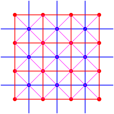
Figure 2: The two dimensional lattice structure of the ${\cal Q}=0$ link(2) lattice formulation of ${\cal N}=(2,2)$ target theory. The lattice can be split into even (red) and odd (blue) sublattices. The bosonic degrees of freedom reside on red and blue links. The fermions reside on the diagonal magenta links. This lattice theory can be obtained by a non-supersymmetric orbifold projection of the ${\cal N}=(2,2)$ matrix model. There are no dynamical fields residing on the sites.

$$S^{\rm link(2)}= \frac{1}{g^{2}}\sum_{{\bf n}}\operatorname{Tr}\Big{[}{\textstyle{\frac{1}{2}}}\Big{(}\bar{z}_{1}({\bf n}-2{\bf e}_{1})z_{1}({\bf n}-2{\bf e}_{1})-z_{1}({\bf n})\bar{z}_{1}({\bf n})+(1\leftrightarrow 2)\Big{)}^{2}$$ (132)

$$+2\Big{|}z_{1}({\bf n})z_{2}({\bf n}+2{\bf e}_{1})-z_{2}({\bf n})z_{1}({\bf n}+2{\bf e}_{2})\Big{|}^{2}$$

$$+\sqrt{2}\left(\Delta_{\bf n}(\alpha_{12},\bar{z}_{1},\alpha_{1\bar{2}})+\Delta_{\bf n}(\alpha_{12},\bar{z}_{2},\alpha_{\bar{1}2})+\Delta_{\bf n}(\alpha_{\bar{1}\bar{2}},z_{1},\alpha_{\bar{1}2})-\Delta_{\bf n}(\alpha_{\bar{1}\bar{2}},z_{2},\alpha_{1\bar{2}})\right)\Big{]}\qquad\qquad$$

where we have used the triangular plaquette function $\Delta_{\bf n}$ given by

$$\Delta_{\bf n}(\alpha_{12},\bar{z}_{1},\alpha_{1\bar{2}})=\alpha_{12}({\bf n})\Big{(}\bar{z}_{1}({\bf n}-{\bf e}_{1}+{\bf e}_{2})\alpha_{1\bar{2}}({\bf n}-{\bf e}_{1}+{\bf e}_{2})-\alpha_{1\bar{2}}({\bf n}+{\bf e}_{1}+{\bf e}_{2})\bar{z}_{1}({\bf n})\Big{)}\qquad\qquad$$ (133)

(134)

$$\Delta_{\bf n}(\alpha_{12},\bar{z}_{2},\alpha_{\bar{1}2})=\alpha_{12}({\bf n})\Big{(}\bar{z}_{2}({\bf n}+{\bf e}_{1}-{\bf e}_{2})\alpha_{\bar{1}2}({\bf n}+{\bf e}_{1}-{\bf e}_{2})-\alpha_{\bar{1}2}({\bf n}+{\bf e}_{1}+{\bf e}_{2})\bar{z}_{2}({\bf n})\Big{)}\qquad\qquad$$ (135)

(136)

$$\Delta_{\bf n}(\alpha_{\bar{1}\bar{2}},z_{1},\alpha_{\bar{1}2})=\alpha_{\bar{1}\bar{2}}({\bf n})\Big{(}z_{1}({\bf n}-{\bf e}_{1}-{\bf e}_{2})\alpha_{\bar{1}2}({\bf n}+{\bf e}_{1}-{\bf e}_{2})-\alpha_{\bar{1}2}({\bf n}-{\bf e}_{1}-{\bf e}_{2})z_{1}({\bf n}-2{\bf e}_{1})\Big{)}\qquad$$ (137)

(138)

$$\Delta_{\bf n}(\alpha_{\bar{1}\bar{2}},z_{2},\alpha_{1\bar{2}})=\alpha_{\bar{1}\bar{2}}({\bf n})\Big{(}z_{1}({\bf n}-{\bf e}_{1}-{\bf e}_{2})\alpha_{1\bar{2}}({\bf n}-{\bf e}_{1}+{\bf e}_{2})-\alpha_{1\bar{2}}({\bf n}-{\bf e}_{1}-{\bf e}_{2})z_{2}({\bf n}-2{\bf e}_{2})\Big{)}\qquad$$ (139)

This is the link(2) action studied in [39]. In the discussion of the representation theory of point group symmetry, we ignore lattice site index ${\bf n}$ for convenience.

The ${\cal Q}=0$ link(2) formulation of the ${\cal N}=(2,2)$ has a $D_{4}$ point group symmetry with order eight. These are the full set of symmetry operations of a square and are shown in Table.1.

classes: ($e$) (2$C_{4}$) ($C_{2}$) (2 $C_{2}^{\prime}$) (2$C_{2}^{\prime\prime}$) $A_{1}$ 1 1 1 1 1 $A_{2}$ 1 1 1 -1 -1 $B_{1}$ 1 -1 1 1 -1 $B_{2}$ 1 -1 1 -1 1 $E$ 2 0 -2 0 0

Table 1: The character table of $D_{4}$, the point symmetry group of two dimensional link(2) lattice formulation for ${\cal N}=(2,2)$ theory [39]. $e$ is identity, $C_{4}$ and $C_{2}$ are rotations by $\pi/4$ and $\pi/2$, $C_{2}^{\prime}$ are reflections with respect to ${\bf e}_{1}$ and ${\bf e}_{2}$ axis, and $C_{2}^{\prime\prime}$ are reflections with respect to diagonals, ${\bf e}_{1}\pm{\bf e}_{2}$.

This should be contrasted with the $Z_{2}$ point group symmetry of the ${\cal Q}=1$ supersymmetry preserving regularization of the ${\cal N}=(2,2)$ SYM theory [11]. The apparent trade-off here is between supersymmetry and point group symmetry. In link(2), one achieves much larger point group symmetry $D_{4}$ to the price of giving up the exact lattice supersymmetry.

One other interpretational distinction relative to [39] that we wish to emphasize is that, the link fermions are not the natural implementation of the Dirac-Kähler decomposition on lattice (although see the appendix of [37]). In particular, in link(2) formulation, all the fermions are on the same footing. They do transform to one another under $\pi/4$ rotations, and this is also an invariance of action. However, in a natural implementation of Dirac-Kähler fermions, the fermions are one zero form $\psi^{(0)}$, two one-form $\psi^{(1)}$ and one two-form $\psi^{(2)}$ . Obviously, no lattice rotation can map a zero form $\psi^{(0)}$ to a one-form $\psi^{(1)}$ or vice-versa. Therefore, in what sense, the link(2) formulation is related to the Dirac-Kähler fermions? One other related puzzle: Obviously, $\psi^{(0)}$ is a scalar under $SO(2)^{\prime}$. Therefore, it must be in a scalar representation of any discrete subgroup $G_{\rm point}$ of $SO(2)^{\prime}$. How does this reconcile with the link nature of all the fermions?

In order to answer these questions, we classify the fields on the lattice in terms of the irreducible representations of $D_{4}$. We expect the irreducible representations under $D_{4}$ to have a natural interpretation under $SO(2)^{\prime}$. To do so, we consider the action of the elements of $D_{4}$ (one from each conjugacy class) on the lattice fields, and then evaluate the character of the operation. The action of $g\in D_{4}$ on elements of a unit cell is given by

$$(e):(\alpha_{12},\alpha_{\bar{1}2},\alpha_{\bar{1}\bar{2}},\alpha_{1\bar{2}}),\;\;(z_{1},z_{2})\rightarrow(\alpha_{12},\alpha_{\bar{1}2},\alpha_{\bar{1}\bar{2}},\alpha_{1\bar{2}}),\;\;(z_{1},z_{2})$$ (140)

(141)

$$C_{4}:\qquad\qquad\qquad\qquad\qquad\qquad\;\;\rightarrow(\alpha_{\bar{1}2},\alpha_{\bar{1}\bar{2}},\alpha_{1\bar{2}},\alpha_{12}),\;\;(z_{2},\bar{z}_{1})$$ (142)

(143)

$$C_{2}:\qquad\qquad\qquad\qquad\qquad\qquad\;\;\rightarrow(\alpha_{\bar{1}\bar{2}},\alpha_{1\bar{2}},\alpha_{12},\alpha_{\bar{1}2}),\;\;(\bar{z}_{1},\bar{z}_{2})$$ (144)

(145)

$$C_{2}^{\prime}:\qquad\qquad\qquad\qquad\qquad\qquad\;\;\rightarrow(\alpha_{1\bar{2}},\alpha_{\bar{1}\bar{2}},\alpha_{\bar{1}2},\alpha_{12}),\;\;(z_{1},\bar{z}_{2})$$ (146)

(147)

$$C_{2}^{\prime\prime}:\qquad\qquad\qquad\qquad\qquad\qquad\;\;\rightarrow(\alpha_{12},\alpha_{1\bar{2}},\alpha_{\bar{1}\bar{2}},\alpha_{\bar{1}2}),\;\;(z_{2},z_{1})$$ (148)

The character is $\chi(g)=\operatorname{Tr}(M(g))$, where $M(g)$ is a matrix representation of the operation $g$. Since the character is a class function, it is independent of representative. Thus, we make a character multiplet $\left[\chi(M(e)),\ldots,\chi(M(C_{2}^{\prime\prime}))\right]$. For the fermions, the hermitian $\Re({\rm bosons})$ and anti-hermitian $\Im({\rm bosons})$ components of link bosons, we obtain

$$\chi^{\rm fermions}=[4,0,0,0,2]=A_{1}\oplus B_{2}\oplus E$$ (149)

(150)

$$\chi^{\Re(\rm bosons)}=[2,0,2,2,0]=A_{1}\oplus B_{1}$$ (151)

(152)

$$\chi^{\Im(\rm bosons)}=[2,0,-2,0,0]=E$$ (153)

The gauge bosons [$\Im({\rm bosons})$] and scalars [$\Re({\rm bosons})$] respectively fill in vector and pseudo-vector representation of the twisted $SO(2)^{\prime}$. Under the $D_{4}$ subgroup, there is a two dimensional irreducible representation $E$ corresponding to vectors. The pseudo-vector is reducible and splits as $A_{1}\oplus B_{1}$. The fermions apparently form a reducible representation and split into two one dimensional representations ($A_{1}$ and $B_{2}$) and a two dimensional vector representation $E$. We can indeed identify the irreducible representations of $D_{4}$ with the natural realization of the Dirac-Kähler fermions on the lattice, for example, the zero-form $\psi^{(0)}\sim\frac{1}{2}(\alpha_{12}+\alpha_{\bar{1}2}+\alpha_{\bar{1}\bar{2}}+\alpha_{1\bar{2}})$ where the right hand side corresponds to $A_{1}$. Thus, the irreducible representation of the $D_{4}$ nicely maps into the Dirac-Kähler twisted version of continuum, with twisted rotation group $SO(2)^{\prime}$. In other words,

$$A_{1}\oplus E\oplus B_{2}\sim\psi^{(0)}\oplus\psi^{(1)}\oplus\psi^{(2)}\sim 1\oplus 2\oplus 1$$ (154)

Similar phenomena also takes place in supersymmetric $A_{d}^{*}$ lattices where the decomposition of link and face fermions into the irreducible representations under the permutation group $S_{d+1}^{\prime}\subset SO(d)^{\prime}$ results in the usual Dirac-Kähler decomposition. This is also how the link(2) lattice produces the Dirac-Kähler twist in its continuum.

Remark: The gauging of the Dirac-Kähler fermions and link fermions are also different. For example, although the $\frac{1}{2}(\alpha_{12}+\alpha_{\bar{1}2}+\alpha_{\bar{1}\bar{2}}+\alpha_{1\bar{2}})$ is a singlet under $D_{4}$, it cannot be contracted with any other $D_{4}$ singlet to form a relevant (or irrelevant) gauge singlet operator at any finite lattice spacing. The reason is, in the gauged lattice theory, $(\alpha_{12}+\alpha_{\bar{1}2}+\alpha_{\bar{1}\bar{2}}+\alpha_{1\bar{2}})$ does not transform co-variantly under gauge rotations. Let $G({\bf n})$ denote a gauge rotation associated with site ${\bf n}$. Then, under a gauge transformation, the constituents transform as

$$\alpha_{12}({\bf n})\rightarrow G({\bf n})\;\alpha_{12}({\bf n})\;G^{\dagger}({{\bf n}+{\bf e}_{1}+{\bf e}_{2}}),\qquad\alpha_{\bar{1}2}({\bf n})\rightarrow G({\bf n})\;\alpha_{\bar{1}2}({\bf n})\;G^{\dagger}({\bf n}-{\bf e}_{1}+{\bf e}_{2}),$$ (155)

$$\alpha_{1\bar{2}}({\bf n})\rightarrow G({\bf n})\;\alpha_{1\bar{2}}({\bf n})\;G^{\dagger}({\bf n}+{\bf e}_{1}-{\bf e}_{2}),\qquad\alpha_{\bar{1}\bar{2}}({\bf n})\rightarrow G({\bf n})\;\alpha_{\bar{1}\bar{2}}({\bf n})\;G^{\dagger}({{\bf n}-{\bf e}_{1}-{\bf e}_{2}}).$$ (156)

This means, the combination of gauge invariance and $D_{4}$ symmetry is vastly more restrictive than each would be individually. The combination restricts the type of operators that one can write down. This also shows that, at finite lattice spacing, the link fermions and Dirac-Kähler implementation are truly different. For example, the zero form site fermion transform by conjugation, $\psi^{(0)}({\bf n})\rightarrow G({\bf n})\;\psi^{(0)}({\bf n})\;G^{\dagger}({{\bf n}})$. Of course, in classical continuum limit, this difference is lifted, since all the fermion and boson fields transform as adjoints.

Comments on classical and quantum continuum limits: Consider the classical and quantum continuum limit of the link(2) formulation. In the classical continuum limit,

$$S^{\rm link(2)}=S^{{\cal N}=(2,2)}[1+O(aq)]$$ (157)

where $S^{{\cal N}=(2,2)}$ is the action for the continuum ${\cal N}=(2,2)$ theory, and $q$ is some Euclidean momenta.

We wish to understand the quantum continuum limit of these theories when the radiative corrections are taken into account. (Below, we follow the analysis of §5 of Ref.[11] verbatim.) Consider a radiative correction to the action of an operator ${\cal O}$ with dimension $p$

$$\delta S=\frac{1}{g_{2}^{2}}\int d^{2}xC_{\cal O}{\cal O}$$ (158)

Since the lattice theory is a ${\cal Q}=0$ theory, there is no integration over a superspace coordinate. In power counting, we use the classical scaling dimensions, $[dx]=-1,\;[{\rm bosons}]=+1,\;[{\rm fermions}]=+3/2,\;[g_{2}^{2}]=+2$, and $a$ is the lattice spacing. By [11], the coefficient $C_{\cal O}$ has a loop expansion

$$C_{\cal O}=a^{p-4}\sum_{\ell}c_{\ell}(g_{2}^{2}a^{2})^{\ell}$$ (159)

where $c_{\ell}$ may have logarithmic dependence on the lattice spacing $a$.

The operators for which $p-4+2\ell\leq 0$ are the only possible local counter-terms. At classical $\ell=0$ level, the long distance action for the lattice theory agrees with the target theory, as shown in eq. (157). For $l\geq 2$, there are no local relevant or marginal counter-terms that get induced radiatively. However, for $\ell=1$, the scalar mass operator with $p=2$ may receive a logarithmic correction.

This is unlike the ${\cal Q}=1$ supersymmetric lattice [11]. In that case, only the counter-terms with $p-7/2+2\ell\leq 0$ are possible due to exact supersymmetry and the scalar mass operator does not get induced radiatively.

The scalar mass operator is a relevant operator which does affect the physics of the target theory, and it is allowed by all the symmetries of the link(2) lattice action. Is it, however, possible that an operator which is allowed by all the symmetries of the microscopic theory may not be generated? Or is there a reason to think that the behavior of these theories in the continuum may be tamer than the above analysis suggests? Naively, the spectrum of fermions and bosons are degenerate even at a finite lattice spacing, and the number of degrees of freedom of both types is balanced. For each fermionic loop, there is a bosonic loop and vice versa. Moreover, the eq. (157) implies that the interaction vertices of the theory defined by $S^{\rm link(2)}$, close to the continuum limit, may be expressed as

$$V^{\rm lattice}=V^{\rm cont.}[1+O(qa)]$$ (160)

When inserted into loops, the leading term really just behaves like the extended supersymmetric theory and the correction has an extra suppression factor relative to eq. (159). Perhaps, despite the absence of any supersymmetry at the cut-off, these features may be sufficient to suppress dangerous relevant operators. That would be another way to have naturally light scalars without microscopic supersymmetry or shift symmetry, and would be remarkable.

However, the above line of reasoning may be too naive. In a lattice gauge theory and effective theories, there are cases in which a naively irrelevant operator becomes important and generates unwanted relevant operators. Such behavior may occur if the lower dimension relevant operator is not protected by a symmetry. The best known example, which has a resemblance to the above discussion, is about the chiral symmetry on the lattice and Wilson fermions [35]. The Wilson’s lattice fermion Lagrangian is

$$\kern 0.6pt\overline{\kern-0.6pt\psi\kern-0.6pt}\kern 0.6pt(i\gamma_{\mu}D_{\mu}-m-ar\Delta)\psi$$ (161)

where $D_{\mu}$ and $\Delta$ are gauge covariant Dirac-operator and Laplacian, $a$ is lattice spacing, $m$ is bare mass and $r$ is an order one parameter introduced to lift the spurious doublers. In the naive continuum limit, the operator proportional to lattice spacing is an irrelevant dimension five operator. Both $m$ and $r$ terms explicitly violate the chiral symmetry. In this theory, the fermion mass term, instead of being multiplicatively renormalized, is additively renormalized by a term proportional to $r/a$. Thus, the naively irrelevant dimension five operator radiatively induces a dimension three operator. If the target theory is massless or a theory with a light fermion, the exact or approximate chiral symmetry of the naive continuum limit is spoiled by a so called “irrelevant” operator.

The danger in the link(2) formulation is analogous. There is no symmetry which protects scalar masses in these formulations in general. The naive classical continuum limit has supersymmetry. What one really needs to check are the higher dimension, irrelevant operators which may generate the scalar mass operator when inserted into loops. Perhaps, just like the absence of the chiral symmetry does not admit naturally light fermions, the absence of the exact supersymmetry does not admit light scalars either. To sum up, we are inconclusive about the amount of fine-tuning in the quantum continuum limit of the ${\cal Q}=0$ link(2) theory.

6.2.2 Representation theory for the twisted full octahedral group

The matter content of the ${\cal Q}=0$ link(2) lattice for the $d=3$ dimensional ${\cal N}=4$ SYM target theory is as follows: On a unit cell, there are three types of complexified bosonic fluctuations $(z_{1},z_{2},z_{3})$ (and their conjugates) and eight types of Grassmann fields $\alpha_{123},\alpha_{\bar{1}23},\ldots$ etc. The fermions reside on the links

$$\alpha_{123}:{\bf 0}\rightarrow+{\bf e}_{1}+{\bf e}_{2}+{\bf e}_{3}\qquad\alpha_{\bar{1}\bar{2}\bar{3}}:{\bf 0}\rightarrow-{\bf e}_{1}-{\bf e}_{2}-{\bf e}_{3}\qquad$$ (162)

$$\alpha_{1\bar{2}\bar{3}}:{\bf 0}\rightarrow+{\bf e}_{1}-{\bf e}_{2}-{\bf e}_{3}\qquad\alpha_{\bar{1}23}:{\bf 0}\rightarrow-{\bf e}_{1}+{\bf e}_{2}+{\bf e}_{3}\qquad$$ (163)

$$\alpha_{\bar{1}2\bar{3}}:{\bf 0}\rightarrow-{\bf e}_{1}+{\bf e}_{2}-{\bf e}_{3}\qquad\alpha_{1\bar{2}3}:{\bf 0}\rightarrow+{\bf e}_{1}-{\bf e}_{2}+{\bf e}_{3}\qquad$$ (164)

$$\alpha_{\bar{1}\bar{2}3}:{\bf 0}\rightarrow-{\bf e}_{1}-{\bf e}_{2}+{\bf e}_{3}\qquad\alpha_{12\bar{3}}:{\bf 0}\rightarrow+{\bf e}_{1}+{\bf e}_{2}-{\bf e}_{3}\qquad$$ (165)

and the bosons are associated with

$$z_{1}:{\bf 0}\rightarrow+2{\bf e}_{1}\qquad\qquad z_{2}:{\bf 0}\rightarrow+2{\bf e}_{2}\qquad\qquad z_{3}:{\bf 0}\rightarrow+2{\bf e}_{3},$$ (166)

The point group symmetry is the full octahedral group $O_{h}=O\ltimes I$ where $O$ is the pure rotations and $I$ is the inversion. Hence, $O_{h}$ has both proper and improper rotations. The 48 group operations and the character table are shown in Table.2.

classes: ($e$) (8$C_{3}$) ($3C_{2}$) (6 $C_{2}^{\prime}$) (6$C_{4}$) ($i$) (8$S_{3}$) ($3S_{2}$) (6 $S_{2}^{\prime}$) (6$S_{4}$) $A_{1g}$ 1 1 1 1 1 1 1 1 1 1 $A_{2g}$ 1 1 1 -1 -1 1 1 1 -1 -1 $E_{g}$ 2 -1 2 0 0 2 -1 2 0 0 $T_{1g}$ 3 0 -1 -1 1 3 0 -1 -1 1 $T_{2g}$ 3 0 -1 1 -1 3 0 -1 1 -1 $A_{1u}$ 1 1 1 1 1 -1 - 1 - 1 - 1 - 1 $A_{2u}$ 1 1 1 -1 -1 -1 -1 -1 1 1 $E_{u}$ 2 -1 2 0 0 -2 1 -2 0 0 $T_{1u}$ 3 0 -1 -1 1 -3 0 1 1 -1 $T_{2u}$ 3 0 -1 1 -1 -3 0 1 -1 1

Table 2: The character table of full octahedral group $O_{h}$, the point symmetry group of the three dimensional link(2) lattice formulation for ${\cal N}=4$ (or ${\cal Q}=8$) target theory [40]. $e$ is identity, $8C_{3}$ are rotations by $2\pi/3$ along the body-diagonals, $3C_{2}$ and $6C_{4}$ are rotations by $\pi/2$ and $\pi/4$ along the line passing through the center of faces, $6C_{2}^{\prime}$ are rotations by $\pi$ along the lines cutting the edges in the middle. $i$ is inversion, and $S=C\times i$. The character table of $O_{h}$ can be deduced from the product of octahedral group $O$ (upper-left five by five block) and the $I$ inversion group.

As in the two dimensional example, we wish to understand the representations of various lattice fields and decompose them into their irreducible representations. It is sufficient to first inspect the action of $g\in O$ subgroup of $O_{h}$ on the fields on a unit cell

$$(e)\;\;\;\;:\rightarrow(\alpha_{123},\alpha_{1\bar{2}\bar{3}},\alpha_{\bar{1}2\bar{3}},\alpha_{\bar{1}\bar{2}3},\alpha_{\bar{1}\bar{2}\bar{3}},\alpha_{\bar{1}23},\alpha_{1\bar{2}3},\alpha_{12\bar{3}}),\;\;(z_{1},z_{2},z_{3})$$ (167)

(168)

$$(8C_{3}):\rightarrow(\alpha_{231},\alpha_{2\bar{3}\bar{1}},\alpha_{\bar{2}3\bar{1}},\alpha_{\bar{2}\bar{3}1},\alpha_{\bar{2}\bar{3}\bar{1}},\alpha_{\bar{2}31},\alpha_{2\bar{3}1},\alpha_{23\bar{1}}),\;\;(z_{2},z_{3},z_{1})$$ (169)

(170)

$$(3C_{2}):\rightarrow(\alpha_{\bar{1}\bar{2}3},\alpha_{\bar{1}2\bar{3}},\alpha_{1\bar{2}\bar{3}},\alpha_{123},\alpha_{12\bar{3}},\alpha_{1\bar{2}3},\alpha_{\bar{1}23},\alpha_{\bar{1}\bar{2}\bar{3}}),\;\;(\bar{z}_{1},\bar{z}_{2},z_{3})$$ (171)

(172)

$$(6C_{2}^{\prime}):\rightarrow(\alpha_{21\bar{3}},\alpha_{2\bar{1}3},\alpha_{\bar{2}13},\alpha_{\bar{2}\bar{1}\bar{3}},\alpha_{\bar{2}\bar{1}3},\alpha_{\bar{2}1\bar{3}},\alpha_{2\bar{1}3},\alpha_{213}),\;\;(z_{2},z_{1},\bar{z}_{3})$$ (173)

(174)

$$(6C_{4}):\rightarrow(\alpha_{2\bar{1}3},\alpha_{21\bar{3}},\alpha_{\bar{2}\bar{1}\bar{3}},\alpha_{\bar{2}13},\alpha_{\bar{2}1\bar{3}},\alpha_{\bar{2}\bar{1}3},\alpha_{213},\alpha_{2\bar{1}\bar{3}}),\;\;(z_{2},\bar{z}_{1},z_{3})$$ (175)

The inversion $(i)$ acts as

$$(i)\;\;\;\;:\rightarrow(\alpha_{\bar{1}\bar{2}\bar{3}},\alpha_{\bar{1}23},\alpha_{1\bar{2}3},\alpha_{12\bar{3}},\alpha_{123},\alpha_{1\bar{2}\bar{3}},\alpha_{\bar{1}2\bar{3}},\alpha_{\bar{1}\bar{2}3}),\;\;(\bar{z}_{1},\bar{z}_{2},\bar{z}_{3})$$ (176)

Since $O_{h}=O\ltimes I$, the character multiplet $[\chi(M(e)),\ldots,\chi(M(S_{4}))]$ can be deduced by eq. (175) and eq. (176), where $M(g)$ is a matrix representation of the $g\in O_{h}$. By studying the action of $g\in O_{h}$ on fermions, and hermitian and anti-hermitian parts of the bosonic link matrices, the character multiplets can be obtained as

$$\chi^{\rm fermions}=[8,2,0,0,0,0,0,0,4,0]=A_{1g}\oplus T_{2g}\oplus T_{1u}\oplus A_{2u}$$ (177)

(178)

$$\chi^{\Re(\rm bosons)}=[3,0,3,1,1,3,0,3,1,1]=A_{1g}\oplus E_{g}$$ (179)

(180)

$$\chi^{\Im(\rm bosons)}=[3,0,-1,-1,1,-3,0,1,-1,1]=T_{2u}$$ (181)

The gauge boson remains irreducible under $O_{h}\subset SO(3)^{\prime}$ and fills in the three dimensional $T_{2u}$ representation. The scalars are as well in the three dimensional vector representation of twisted $SO(3)^{\prime}$ group, however, they are pseudo-vector as opposed to being vectors. The characters for the inversion operation are $\chi^{\Im(\rm bosons)}(i)=-3$ and $\chi^{\Re(\rm bosons)}(i)=+3$ reflecting vector and pseudo-vector nature of these fields. The pseudo-vector representation of $SO(3)^{\prime}$ is reducible under the $O_{h}$ subgroup, and splits as $A_{1g}\oplus E_{g}$. For fermions, everything works out beautifully. The irreducible representations of the $O_{h}$ map into the Dirac-Kähler twisted version of continuum:

$$A_{1g}\oplus T_{2g}\oplus T_{1u}\oplus A_{2u}\sim\psi^{(0)}\oplus\psi^{(1)}\oplus\psi^{(2)}\oplus\psi^{(3)}\sim 1\oplus 3\oplus 3\oplus 1$$ (182)

Let us reiterate the conclusion of the previous section: Although there is a one to one map between the irreducible representation of $O_{h}$ and Dirac-Kähler decomposition, the gauging of the link fermions and $p$-form fermions are different. Thus, there is no gauge co-variant identification of the various $p$-form lattice fermions and link formulation fermions at any finite lattice spacing. Of course, in the continuum, the discrepancy disappears. This is the sense in which the link fermion approach is tied with the Dirac-Kähler structure of the continuum formulation.

6.3 A ${\cal Q}=0$ deformed matrix model for link(2) formulations

The equality of the number of supersymmetries in the deformed matrix models and supersymmetric orbifold lattices suggests that there must also exist a ${\cal Q}=0$ deformed matrix models which reproduce the non-supersymmetric ${\cal Q}=0$ link(2) lattices. The ${\cal Q}=0$ matrix model for ${\cal N}=(2,2)$ target theory may be found by adapting the techniques of the Ref.[6]. The corresponding non-supersymmetric deformed matrix model action is

$$S^{\rm deformed}=\frac{1}{g^{2}}\operatorname{Tr}\Bigg{[}{\textstyle{\frac{1}{2}}}\Big{(}[\bar{z}_{1},z_{1}]+[\bar{z}_{2},z_{2}]\Big{)}^{2}+2\Big{|}e^{i\beta/2}z_{1}z_{2}-e^{-i\beta/2}z_{2}z_{1}\Big{|}^{2}$$ (183)

$$+\sqrt{2}\left(\alpha_{12}[\bar{z}_{1},\alpha_{1\bar{2}}]_{\beta/4}+\alpha_{12}[\bar{z}_{2},\alpha_{\bar{1}2}]_{-\beta/4}+\alpha_{\bar{1}\bar{2}}[z_{1},\alpha_{\bar{1}2}]_{\beta/4}-\alpha_{\bar{1}\bar{2}}[z_{2},\alpha_{1\bar{2}}]_{-\beta/4}\right)\Bigg{]}\qquad$$ (184)

where

$$[\bar{z}_{1},\alpha_{1\bar{2}}]_{\beta/4}\equiv e^{i{\beta/4}}\;\bar{z}_{1}\alpha_{1\bar{2}}-e^{-i{\beta/4}}\;\alpha_{1\bar{2}}\bar{z}_{1}$$ (185)

For $\beta=0$, the action is the dimensional reduction of the $d=4$ ${\cal N}=1$ SYM theory down to $d=0$ and possesses ${\cal Q}=4$ supersymmetries. For $\beta\neq 0$, the eq. (184) possesses no fermionic symmetry at all. This can be seen explicitly by computation. For example,

$$Qz_{1}=\sqrt{2}\alpha_{1\bar{2}}\qquad\qquad\qquad\qquad\qquad Q\bar{z}_{1}=0$$ (186)

$$Qz_{2}=\sqrt{2}\alpha_{\bar{1}2}\qquad\qquad\qquad\qquad\qquad Q\bar{z}_{2}=0$$ (187)

$$Q\alpha_{12}=-[\bar{z}_{1},z_{1}]-[\bar{z}_{2},z_{2}]\qquad\qquad\;\;Q\alpha_{1\bar{2}}=0$$ (188)

$$Q\alpha_{\bar{1}\bar{2}}=2[\bar{z}_{1},\bar{z}_{2}]\qquad\qquad\qquad\qquad\;\;\;\;Q\alpha_{\bar{1}2}=0.$$ (189)

is an on-shell supersymmetry of the undeformed theory, the one given in Ref.[11]. But this is not a supersymmetry of the deformed action given in eq. (184). This is also true for all four supersymmetries or any linear combination thereof.

It is in fact transparent that the eq. (184) cannot have any of the fermionic symmetries of the undeformed theory. One reason is the mismatch of the $\beta$ commutators in the bosonic and fermionic parts of the action. The form of the deformed action in the fermionic terms is

$$S_{f}\sim\alpha_{12}[\bar{z}_{1},\alpha_{1\bar{2}}]_{\beta/4}=e^{i{\beta/4}}\alpha_{12}\bar{z}_{1}\alpha_{1\bar{2}}-e^{-i{\beta/4}}\alpha_{12}\alpha_{1\bar{2}}\bar{z}_{1},\qquad$$ (190)

whereas, for example, the second bosonic term is

$$S_{b}\sim|[z_{1},z_{2}]_{\beta/2}|^{2}=z_{1}z_{2}\bar{z}_{2}\bar{z}_{1}+z_{2}z_{1}\bar{z}_{1}\bar{z}_{2}-e^{i{\beta}}z_{1}z_{2}\bar{z}_{1}\bar{z}_{2}-e^{-i{\beta}}z_{2}z_{1}\bar{z}_{2}\bar{z}_{1}$$ (191)

The variation of action under a supersymmetry transformation of the undeformed theory fails to vanish, because various terms which are supposed to cancel multiply different phase factors, for example $e^{\pm i\beta/4}$ versus $e^{\pm i\beta}$. Thus, the action shown in eq. (184) is a ${\cal Q}=0$ non-supersymmetric deformation of the ${\cal Q}=4$ matrix model.

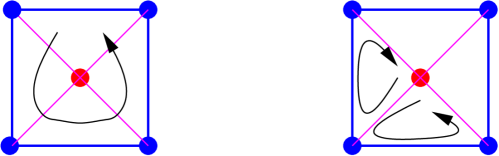
Figure 3: Examples of oriented square and triangular plaquettes. If there is a background field, the net flux passing through the square is four times (in magnitude) the one of triangle. If the theory is reduced to a single point by using the twisted boundary conditions of ’t Hooft, it produces the action with a $e^{\pm i\beta}$ phase for the reduction of square plaquettes, and $e^{\pm i\beta/4}$ phase for the triangle plaquettes.

There is also a nice physical interpretation for the difference of the various phase factors as discussed in detail in supersymmetric case in Ref.[6]. The deformed matrix model eq. (184) can be obtained from the eq. (132), by dimensionally reducing the lattice action to a single point on the lattice by using the ’t Hooft’s twisted boundary conditions for lattice fields. This is a dimensional reduction on lattice with a background flux. In Fig.2 and eq. (132), there are three types of plaquettes that enters into the action, with counter-clockwise and clock-wise orientations. These are square plaquettes with area $4a^{2}$, triangular plaquettes with area $a^{2}$ and flipped-L plaquettes with zero-area [18]. In the reduction with background flux, the phase factors appearing in the reduced matrix model are the fluxes passing through the corresponding surface prior to the reduction. See Fig.3. These corresponds to the phases $e^{\pm i\beta/4}$, $e^{\pm i\beta}$, for triangular and square plaquettes, and identity otherwise.

More specifically, consider the eq. (184) with $U(2Nk)$ algebra valued Grassmann odd and even matrices and $\beta=4\frac{2\pi}{2N}$. Both choices are for the convenience of the presentation. Then, the background and fluctuations of the ${\cal Q}=0$ matrix model can be transmuted into a lattice gauge theory on a $(2N)^{2}$ non-commutative lattice with $U(k)$ gauge group. The resulting action is a familiar one, and gives

$$S^{\rm deformed}=S^{\rm link(2)}|_{\star}.$$ (192)

where $S^{\rm link(2)}|_{\star}$ is same as in eq. (132) with the modification of ordinary product into a $\star$-product. As discussed in §5.0.1, the commutative and non-commutative gauge theories carry equal amount of supersymmetries so long as no deformation in the Grassmann odd space is introduced as done in [53]. Thus, $S^{\rm link(2)}|_{\star}$ has as much global supersymmetries as $S^{\rm link(2)}$, which implies a ${\cal Q}=0$ formulation.

7 Supersymmetric lattice (SL)-twists and topological field theories

There are currently three types of proposal for a non-perturbative formulation of four dimensional ${\cal N}=4$ SYM theory. These are

• Exact Lattice supersymmetry [Orbifold, geometric, Dirac-Kähler, topological field theory motivated Refs.[43, 21, 25]]

• Approaches with no microscopic supersymmetry [with Ginsparg-Wilson fermions [8], link(2) of Ref.[39] with the re-interpretation of §6.1]

• Supersymmetric/non-supersymmetric deformed matrix models, Ref.[6] and generalization of §6.3

Although having a non-perturbative definition of a supersymmetric gauge theory is important in its own right, it is expected that the broader applications of these lattices will be via gauge-gravity duality. A lattice definition of the various sixteen supercharge theories may open up a non-perturbative window into quantum gravity, string theory, and in the large $N$ limit into supergravity. There are however two practical obstacles on the way: the fermion sign problem and the amount of fine tuning. In four dimensional supersymmetric lattices, the amount of fine-tuning is still not fully understood, however, it is believed to be surmountable. In $d\leq 3$, no fine tuning is necessary [10]. If these theories can be solved numerically, this will necessitate going beyond what is currently known in supergravity, which is mostly limited to two point functions and thermal behavior as emphasized recently in [59]. In this section, we will not make remarks on the numerical investigations of supersymmetric theories which is already ongoing (See for example, [60, 61, 62].). Rather, we wish to address where SL-twists fit within the class of all twisted supersymmetric theories, and their interrelation to topological theories.

Recent studies on lattice supersymmetry showed that supersymmetric lattices in their continuum limit, always give the twisted version of the supersymmetric theories. These are non-topological physical theories. However, if desired, one can make them topological by declaring the scalar supercharge $Q$ as a BRST operator, and consider only the states $|\Omega\rangle$ annihilated by $Q$ as physical, i.e., $Q|\Omega\rangle=0$, modulo those which can be written as $|\Omega^{\prime}\rangle\sim Q|\Omega^{\prime\prime}\rangle$. In this sense, there is also an intimate connection between the topological field theories and supersymmetric lattices.

A common tread in both topological field theory and lattice supersymmetry is the existence of a nil-potent scalar supercharge $Q$. However, although all supersymmetric lattices may correspond to the twisted version topological field theories (in the above sense), the reverse statement is not true. Given a supersymmetric twist with a scalar supercharge, we are not guaranteed to have a (non-problematic) supersymmetric lattice formulation. Below, we examine this in connection with the twists of the ${\cal N}=4$ SYM theory in $d=4$.

7.1 Three twists of ${\cal N}=4$ SYM in $d=4$: Why SL-twist is special?

The ${\cal N}=4$ SYM theory in $d=4$ has three inequivalent twists, i.e, three inequivalent embedding of an $SU(2)\times SU(2)$ into $SU(4)_{\cal R}$ symmetry, each of which results in one or two scalar supersymmetries [46]. These classes are most easily described by providing the decomposition of ${\bf 4}$ of $SU(4)$ in eq. (71).

$$i)\;\;({\bf 2,1})\oplus({\bf 1,2}),\qquad({\rm SL-twist})$$ (193)

$$ii)\;\;({\bf 1,2})\oplus({\bf 1,2})$$ (194)

$$iii)\;\;({\bf 1,2})\oplus({\bf 1,1})\oplus({\bf 1,1})$$ (195)

Under these embedding, the supercharges (and fermions) transform as

$$i)\;\;{\rm fermions}\; \rightarrow({\bf 1,1})\oplus({\bf 2,2})\oplus[({\bf 3,1})\oplus({\bf 1,3})]\oplus({\bf 2,2})\oplus({\bf 1,1})$$ (198)

$$\rightarrow{\bf 1\oplus 4\oplus 6\oplus 4\oplus 1}\qquad({\rm SL-twist})\;$$

$$ii)\;\;{\rm fermions}\; \rightarrow 2\times\Big{[}{\bf(1,1)\oplus(2,2)\oplus(3,1)}\Big{]}$$ (200)

$$iii)\;\;{\rm fermions}\; \rightarrow\Big{[}{\bf(1,1)\oplus(2,2)\oplus(3,1)}\Big{]}\oplus 2\times\Big{[}({\bf 2,1})\oplus({\bf 1,2})\Big{]}$$ (202)

under the twisted rotation group

$$[SU(2)_{L}\times SU(2)_{R}]^{\prime}\times(G_{a})\subset[SU(2)_{L}\times SU(2)_{R}]\times SU(4)_{\cal R}$$ (203)

where class-dependent global ${\cal R}$-symmetry factor $G_{a}$ $(a=i,ii,iii)$ is not important for our purpose. The gauge boson, which is a $SU(4)$ singlet, transforms as $(\bf 2,2)$. The scalars are singlet under the Lorentz symmetry and is in ${\bf 6}={\bf 4}\wedge{\bf 4}$, anti-symmetric representation of $SU(4)$. Therefore, eq. (195) uniquely fixes the decomposition of ${\bf 6}$ under the twisted rotation group, for example,

$$i)\;\;[({\bf 2,1})\oplus({\bf 1,2})]\wedge[({\bf 2,1})\oplus({\bf 1,2})]=({\bf 2},{\bf 2})\oplus 2({\bf 1,1}),$$ (204)

and similarly,

$$ii)\;\;3({\bf 1,1})\oplus({\bf 1,3})\qquad iii)\;\;2({\bf 1,2})\oplus 2(1,1)$$ (205)

As stated above, all three twists support the existence of at least one nil-potent scalar supercharge $Q\sim({\bf 1,1})$, with $Q^{2}=0$, modulo gauge rotations. The first two has two and the last has one. One would naively expect that, since $Q^{2}=0$ does not interfere with any translation, it should be implementable on the lattice. This intuition is not completely correct. The reason is, what is allowed and what is not in a lattice regularization of supersymmetric theories has a number of other constraints. The existence of a nil-potent supercharge $Q$ in twisted version is not sufficient.

First, note that, all three twists have a copy of the twist of ${\cal N}=2$ SYM theory in $d=4$ [1] where eight supercharges decompose as ${\bf(1,1)\oplus(2,2)\oplus(3,1)}$. This structure exists in a $L^{\prime}\leftrightarrow R^{\prime}$ symmetric manner in the first twist and asymmetric for the last two. This means that, in case $i)$, instead of self-dual two-forms, we can just think of two-forms, without self-duality condition. In lattice gauge theory, the implementation of the self-duality condition in a manifestly gauge covariant fashion is problematic. For example, in continuum, we will have $Q\psi^{\mu\nu,+}=F^{\mu\nu,+}\equiv F^{\mu\nu}+{\textstyle{\frac{1}{2}}}\epsilon^{\mu\nu\rho\sigma}F_{\rho\sigma}$ where both of $\psi^{\mu\nu,+}$ and $F^{\mu\nu,+}$ are in self-dual ${\bf(3,1)}$ representation. The gauge-covariant implementation of the right-hand side on the lattice is not clear, and hence, the meaning of the left hand side (a self-dual Grassmann) is also unclear. This means, the twist $ii)$ and $iii)$ are not very pleasant from lattice point of view. Furthermore, the $iii)$ case also involves double-valued representation scalars and spinors, which are again in double-valued spinor representations of the lattice point group symmetry and do not have a natural habitat on lattice, unlike the $p$-form $p$-cell mapping.

The supersymmetric (orbifold) lattices always produce the twists which do not involve any self-duality conditions. All the fields are in single-valued integer spin representations, and naturally yields twist i), with $Q(u,v)=Q(1,0)=Q$ or the dual $Q(u,v)=Q(0,1)=*Q^{(4)}$, in the notation of eq. (89).

Remark: In the topological field theory literature, it is sometimes asserted that the twist of type $i)$ did not have any application to physics up until the recent discussion of the dualities of Ref.[52]. Most likely, what is meant here is topological applications. This twist had beautiful realizations and applications in supersymmetric lattices. Moreover, if we move to the application outside the supersymmetric or topological context, we immediately realize that the twist of type $i)$ had the most application of all, in particular in lattice gauge theory. The staggered fermions is the twisted version of the complex representation fermions, and the reduced staggered fermions are the twisting applied to real representation fermions. Both are used practically in numerical QCD and discussed in standard textbooks. However, the language is slightly different. In the next section, I will rephrase the staggered fermions as twisting applied to QCD.

8 Twisting in QCD and staggered fermions

In this section, I rephrase the (reduced) staggered fermions as an elegant application of twisting into QCD. The main point of this section is shown in Fig.1. Needless to say, these theories do not admit a topological interpretation, and the twisted theory is necessarily physical. (Recall that in supersymmetric context, we are free to make that choice and switch between the two.) The discussion below borrows from Refs.[63, 64] and the lecture notes [35]. In particular, the interrelation between reduced staggered fermions and the twists useful in the supersymmetric gauge theories was emphasized to me by D.B. Kaplan.

8.1 Staggered fermions as twisted complex representation fermions

Consider massless QCD on $\mathbb{R}^{4}$ with $N_{f}=4$ complex (for example, fundamental) representation fermions. We label Dirac spinors as

$$\Psi_{I}=\left(\begin{array}[]{c}\psi_{\alpha}\\ \kern 0.6pt\overline{\kern-0.6pt\chi\kern-0.6pt}\kern 0.6pt_{\dot{\alpha}}\end{array}\right)_{I}$$ (208)

and $\kern 0.6pt\overline{\kern-0.6pt\Psi\kern-0.6pt}\kern 0.6pt_{I}$ where $I=1,\ldots,4$ is the flavor index. The theory possesses

$$G_{\rm QCD}=[SU(2)_{L}\times SU(2)_{R}]_{\rm Lorentz}\times[U(4)_{L}\times U(4)_{R}]_{\rm flavor}$$ (209)

space-time and (classical) chiral flavor symmetries. Under $G_{\rm QCD}$, the fermions transform as

$$\psi_{\alpha,I}\sim({\bf 2,1,4,1}),\;\;\;\kern 0.6pt\overline{\kern-0.6pt\chi\kern-0.6pt}\kern 0.6pt_{\dot{\alpha},I}\sim({\bf 1,2,1,4})$$ (210)

It is convenient to use the vector-like sum $U(4)_{V}\sim U(4)_{L+R}$ of the flavor symmetry for our purpose. The Weyl components $\psi_{I}$ ($\kern 0.6pt\overline{\kern-0.6pt\chi\kern-0.6pt}\kern 0.6pt_{I}$) fill in $({\bf 2,1,4})$ and $({\bf 1,2,4})$ under $[SU(2)_{L}\times SU(2)_{R}]_{\rm Lorentz}\times[U(4)_{V}]_{\rm flavor}$. Clearly, the flavor symmetries are sufficiently large such that it can accommodate a copy of Lorentz group, i.e, $SO(4)\subset U(4)_{V}$. Thus, the problem maps into the discussion in §4.1, with twice as much fermion content. The next steps are identical. We use the decomposition of ${\bf 4}$ of $U(4)_{V}$ into $({\bf 2,1})\oplus({\bf 1,2})$ and perform a diagonal embedding

$$SO(4)^{\prime}\sim{\rm Diag}\;\Big{(}SO(4)_{\rm Lorentz}\times SO(4)_{\rm flavor}\Big{)}\;.$$ (211)

Under $SO(4)^{\prime}$, the fermions of the original theory map into integer-spin representations, $p$-forms. In an hyper-cubic lattice whose point group symmetry is a discrete subgroup of $G_{\rm point}\subset SO(4)^{\prime}$, it is natural to associate a $p$-form with a $p$-cell. This is the Dirac-Kähler or geometric representation of fermions in lattice.

The above procedure can equivalently be described as follows: $\Psi_{\Upsilon I}$ is a four by four matrix, where $\Upsilon=1,\ldots 4$ is the Dirac spinor index and $I=1,\ldots 4$ is the flavor index. By using four dimensional Euclidean Dirac-matrices $\gamma_{\mu},\mu=1,\ldots 4$, we can define a basis ${\cal B}$ for $GL(4,\mathbb{C})$ given by

$${\cal B}\equiv\{\Gamma^{A},A=1,\ldots 16\}=\{1,\gamma_{\mu},\gamma_{[\mu\nu]},\gamma_{[\mu\nu\rho]},\gamma_{[\mu\nu\rho\sigma]}\}$$ (212)

where $[\ldots]$ denotes (normalized) anti-symmetrization. ${\cal B}$ forms an orthonormal, complete basis for the $GL(4,\mathbb{C})$. The generators satisfy $\operatorname{Tr}\Gamma^{A}\Gamma^{B}=4\delta^{AB}$. Let us also define

$$\{\psi^{A},A=1,\ldots 16\}\equiv\{\psi,\psi_{\mu},\psi_{[\mu\nu]},\psi_{[\mu\nu\rho]},\psi_{[\mu\nu\rho\sigma]}\}$$ (213)

the collection of $p$-form Grassmann valued fields. Thus, we can write

$$(\Psi)_{\Upsilon I} =\sum_{A=1}^{16}\Gamma^{A}\psi^{A},\qquad\psi^{A}=\frac{1}{4}\operatorname{Tr}[\Psi\Gamma^{A}]$$ (214)

or making the $SO(4)^{\prime}$ transformation properties transparent

$$(\Psi)_{\Upsilon I} =\left(\psi 1+\psi^{\mu}\gamma_{\mu}+\frac{1}{2!}\psi^{\mu\nu}\gamma_{[\mu\nu]}+\frac{1}{3!}\psi^{\mu\nu\rho}\gamma_{[\mu\nu\rho]}+\frac{1}{4!}\psi^{\mu\nu\rho\sigma}\gamma_{[\mu\nu\rho\sigma]}\right)_{\Upsilon I}$$

$$(\kern 0.6pt\overline{\kern-0.6pt\Psi\kern-0.6pt}\kern 0.6pt)_{\Upsilon I} =\left(\kern 0.6pt\overline{\kern-0.6pt\psi\kern-0.6pt}\kern 0.6pt1+\kern 0.6pt\overline{\kern-0.6pt\psi\kern-0.6pt}\kern 0.6pt^{\mu}\gamma_{\mu}+\frac{1}{2!}\kern 0.6pt\overline{\kern-0.6pt\psi\kern-0.6pt}\kern 0.6pt^{\mu\nu}\gamma_{[\mu\nu]}+\frac{1}{3!}\kern 0.6pt\overline{\kern-0.6pt\psi\kern-0.6pt}\kern 0.6pt^{\mu\nu\rho}\gamma_{[\mu\nu\rho]}+\frac{1}{4!}\kern 0.6pt\overline{\kern-0.6pt\psi\kern-0.6pt}\kern 0.6pt^{\mu\nu\rho\sigma}\gamma_{[\mu\nu\rho\sigma]}\right)_{\Upsilon I}$$ (215)

Apparently, the fermions transform as $p$-form integer spin representation of $SO(4)^{\prime}$, and on the lattice, they are naturally associated with the $p$-cells, sites, links, faces, cubes, and hypercubes.

The equivalence between the geometric $p$-form fermions and staggered fermions in ungauged lattice theories is well-know. (The gauging slightly complicates things, we will not go into this detail.) The $p$-form fermions can be mapped onto a lattice with half the spacing as follows: Let ${\bf e}_{\mu},\mu=1,\ldots,4$ denote the four dimensional unit vectors, i.e., $({\bf e}_{\mu})_{\nu}=\delta_{\mu\nu}$. The mapping takes site, link, face, 3-cell and 4-cell fermions into $(0,0,0,0)$, ${\bf e}_{\mu}$, ${\bf e}_{\mu}+{\bf e}_{\nu},\mu\neq\nu$, etc. That is, the fermions are mapped onto the sixteen corners of a hypercube. The lattice periodicity is $2{\bf e}_{\mu}$ in each direction, twice the lattice spacing, as it is always the case with staggered fermions. Each site carries two Grassmann valued fields, one barred and one unbarred.

8.2 Reduced staggered fermions as twisted real representation fermions

If there are $N_{f}$ massless Majorana fermions in a real representation of the gauge group such as adjoint, then the flavor symmetry of the theory is $SU(N_{f})_{\rm flavor}$. For example, for QCD with four adjoint fermions [QCD(adj)], the (classical) symmetries of the theory are

$$G_{\rm QCD(adj)}=[SU(2)_{L}\times SU(2)_{R}]_{\rm Lorentz}\times[SU(4)]_{\rm flavor}\times U(1)_{A}$$ (216)

Note that apart from the anomalous $U(1)_{A}$ factor, this is also the spacetime and flavor symmetry of the ${\cal N}=4$ SYM, where flavor symmetry is called an ${\cal R}$-symmetry:

$$G_{N_{f}=4\rm\;QCD(adj)}=G_{{\cal N}=4\;{\rm SYM}}$$ (217)

up to (unimportant) discrete symmetries. Consequently, (and not surprisingly), the reduced staggered fermions realization of the QCD(adj) is intimately related to the famous twist $i)$ of ${\cal N}=4$ SYM [51, 28, 52]. This twist is also the one which arises naturally in the supersymmetric orbifold lattice [43].

The fermionic matter content of QCD(adj) would be conveniently described by either a Weyl spinor or equivalently, a Majorana spinor:

$$\Psi^{\rm Maj.}_{I}=\left(\begin{array}[]{c}\psi_{\alpha}\\ \kern 0.6pt\overline{\kern-0.6pt\psi\kern-0.6pt}\kern 0.6pt_{\dot{\alpha}}\end{array}\right)_{I}$$ (220)

which fills in

$$\psi_{\alpha,I}\sim({\bf 2,1,4}),\;\;\;\;\;\kern 0.6pt\overline{\kern-0.6pt\psi\kern-0.6pt}\kern 0.6pt_{\dot{\alpha},I}\sim({\bf 1,2,\bar{4}})$$ (221)

representation. The twisting procedure is same as before, where $SU(4)_{\rm flavor}$ replaces the diagonal $SU(4)_{V}$ of the previous section. The final expression is,

$$(\Psi^{\rm M})_{\Upsilon I}=\left(\lambda 1+\psi^{\mu}\gamma_{\mu}+\xi^{\mu\nu}\gamma_{[\mu\nu]}+\xi^{\mu\nu\rho}\gamma_{[\mu\nu\rho]}+\psi^{\mu\nu\rho\sigma}\gamma_{[\mu\nu\rho\sigma]}\right)_{\Upsilon I}$$ (222)

where the same notation as in the ${\cal N}=4$ SYM theory is used to ease the comparison. One can map the geometric $p$-form fermions (which come without unbarred fields) into the reduced staggered fermions as in the previous section. Note that reduced staggered fermions has half as much degree of freedom on the lattice relative to the Kogut-Susskind staggered fermions. This is simply, in the continuum, it corresponds to four flavors of Weyl (or Majorana) spinors as opposed to the four flavors of Dirac spinors. (Compare eq. (215) and eq. (222).)

The cubic supersymmetric orbifold lattices are natural realization of $p$-form Dirac-Kähler fermions and so is the geometric formulation. See for example, [11, 20]. During the writing of [28], it was not fully clear to me what the relation was between these two and the work of Sugino [25], who used reduced staggered fermions in his constructions. The above symmetry arguments also clarify this point. Indeed, Ref.[30, 31] recently constructed a mapping between these formulations at a finite lattice spacing.

9 Discussion

In even space-time dimensions, the deformed matrix models provide an alternative non-perturbative regularization for extended supersymmetric gauge theories, such as ${\cal N}=4$ SYM in $d=4$ and ${\cal N}=(2,2)$ SYM in $d=2$ [6]. These constructions are different from supersymmetric (orbifold) lattices[11], and in particular, the $\beta$-flux deformation cannot be used to fully regularize odd dimensional target theories in a Euclidean setting. However, the matrix model regularization also works for a curved space $S^{2}$, which cannot be obtained via orbifold projections.

Our work also provides a newer interpretation for the link approach [39, 40] to lattice supersymmetry, by benefitting from Ref.[32]. First, we classified the link approach lattices as link(1) [or orbifold(1)] and link(2) [or orbifold(2)]. The first class preserves a (scalar) subset of supersymmetry and the latter preserves none. Despite being non-supersymmetric theories at the cut-off, the link(2)/orbifold(2) class is quite intriguing. They have much larger point group symmetry $G_{\rm point}$ relative to the supersymmetry preserving formulations. In some sense, supersymmetry in the former is traded with the large discrete chiral and discrete space-time symmetry $G_{\rm point}$ realized in ${\rm Diag}(SO(d)_{\rm Lorentz}\times SO(d)_{\rm\cal R})$ in the latter. In the classical continuum limit of the link(2) type lattices, one obtains full extended supersymmetry. Whether this may be achieved in full quantum theory is not clear yet. In particular, there are supersymmetry violating relevant operators, such as mass operators for scalars (which is forbidden in supersymmetric lattices), and it is important to check that higher dimensional operators do not induce them radiatively.

We also demonstrated an equivalence. The supersymmetric deformed matrix models with ${\cal Q}={\rm few}$ produce a supersymmetric lattice gauge theory, both with a commutative and non-commutative continuum limit. At finite lattice spacing, the non-commutative lattice theories have identical actions with the supersymmetric (orbifold) lattices, modulo the substitution of the $\star$-product with the ordinary product of fields. Both formulations respect the same set of supersymmetries. The link(2) formulations can also be obtained from deformed matrix models. The corresponding matrix models are new ${\cal Q}=0$ (non-supersymmetric) $\beta$ flux deformations of supersymmetric matrix models. This equivalence also confirms that the is no exact supersymmetry associated with link(2) constructions.

There are also few other topics that we either rephrased existing results in literature, or we were unable to say much. One is the generality of the concept of twisting. This is a useful notion in QCD via the use of staggered fermions, in (non-topological) physical supersymmetric theories, in lattice gauge theory, and in topological supersymmetric field theories. One direction that can perhaps be improved significantly is the physical interpretation of the ${\cal N}={\textstyle{\frac{1}{4}}}$ SYM theory on $\mathbb{R}^{4}$, and its lower dimensional counterparts.

- [1] E. Witten, Topological Quantum Field Theory, Commun. Math. Phys. 117 (1988) 353.
- [2] J. Kato, N. Kawamoto, and A. Miyake, N = 4 twisted superspace from Dirac-Kaehler twist and off- shell SUSY invariant actions in four dimensions, Nucl. Phys. B721 (2005) 229–286, [hep-th/0502119].
- [3] R. G. Leigh and M. J. Strassler, Exactly marginal operators and duality in four-dimensional N=1 supersymmetric gauge theory, Nucl. Phys. B447 (1995) 95–136, [hep-th/9503121].
- [4] J. Nishimura, S.-J. Rey, and F. Sugino, Supersymmetry on the noncommutative lattice, JHEP 02 (2003) 032, [hep-lat/0301025].
- [5] M. Unsal, Regularization of non-commutative SYM by orbifolds with discrete torsion and SL(2,Z) duality, JHEP 12 (2005) 033, [hep-th/0409106].
- [6] M. Unsal, Supersymmetric deformations of type IIB matrix model as matrix regularization of N = 4 SYM, JHEP 04 (2006) 002, [hep-th/0510004].
- [7] H. Suzuki and Y. Taniguchi, Two-dimensional N = (2,2) super Yang-Mills theory on the lattice via dimensional reduction, JHEP 10 (2005) 082, [hep-lat/0507019].
- [8] J. W. Elliott, J. Giedt, and G. D. Moore, Lattice four-dimensional N=4 SYM is practical, 0806.0013.
- [9] S.-S. Lee, Emergence of supersymmetry at a critical point of a lattice model, Physical Review B 76 (2007) 075103.
- [10] D. B. Kaplan, E. Katz, and M. Unsal, Supersymmetry on a spatial lattice, JHEP 05 (2003) 037, [hep-lat/0206019].
- [11] A. G. Cohen, D. B. Kaplan, E. Katz, and M. Unsal, Supersymmetry on a Euclidean spacetime lattice. I: A target theory with four supercharges, JHEP 08 (2003) 024, [hep-lat/0302017].
- [12] A. G. Cohen, D. B. Kaplan, E. Katz, and M. Unsal, Supersymmetry on a Euclidean spacetime lattice. II: Target theories with eight supercharges, JHEP 12 (2003) 031, [hep-lat/0307012].
- [13] M. G. Endres and D. B. Kaplan, Lattice formulation of (2,2) supersymmetric gauge theories with matter fields, JHEP 10 (2006) 076, [hep-lat/0604012].
- [14] T. Onogi and T. Takimi, Perturbative study of the supersymmetric lattice theory from matrix model, Phys. Rev. D72 (2005) 074504, [hep-lat/0506014].
- [15] K. Ohta and T. Takimi, Lattice formulation of two dimensional topological field theory, Prog. Theor. Phys. 117 (2007) 317–345, [hep-lat/0611011].
- [16] J. Giedt, E. Poppitz, and M. Rozali, Deconstruction, lattice supersymmetry, anomalies and branes, JHEP 03 (2003) 035, [hep-th/0301048].
- [17] J. Giedt, Deconstruction and other approaches to supersymmetric lattice field theories, Int. J. Mod. Phys. A21 (2006) 3039–3094, [hep-lat/0602007].
- [18] M. Unsal, Compact gauge fields for supersymmetric lattices, JHEP 11 (2005) 013, [hep-lat/0504016].
- [19] S. Catterall, Lattice supersymmetry and topological field theory, JHEP 05 (2003) 038, [hep-lat/0301028].
- [20] S. Catterall, A geometrical approach to N = 2 super Yang-Mills theory on the two dimensional lattice, JHEP 11 (2004) 006, [hep-lat/0410052].
- [21] S. Catterall, Lattice formulation of N = 4 super Yang-Mills theory, JHEP 06 (2005) 027, [hep-lat/0503036].
- [22] S. Catterall, Simulations of N = 2 super Yang-Mills theory in two dimensions, JHEP 03 (2006) 032, [hep-lat/0602004].
- [23] F. Sugino, A lattice formulation of super Yang-Mills theories with exact supersymmetry, JHEP 01 (2004) 015, [hep-lat/0311021].
- [24] F. Sugino, Super Yang-Mills theories on the two-dimensional lattice with exact supersymmetry, JHEP 03 (2004) 067, [hep-lat/0401017].
- [25] F. Sugino, Various super Yang-Mills theories with exact supersymmetry on the lattice, JHEP 01 (2005) 016, [hep-lat/0410035].
- [26] F. Sugino, Two-dimensional compact N = (2,2) lattice super Yang-Mills theory with exact supersymmetry, Phys. Lett. B635 (2006) 218–224, [hep-lat/0601024].
- [27] F. Sugino, Lattice Formulation of Two-Dimensional N=(2,2) SQCD with Exact Supersymmetry, 0807.2683.
- [28] M. Unsal, Twisted supersymmetric gauge theories and orbifold lattices, JHEP 10 (2006) 089, [hep-th/0603046].
- [29] S. Catterall, From Twisted Supersymmetry to Orbifold Lattices, JHEP 01 (2008) 048, [0712.2532].
- [30] T. Takimi, Relationship between various supersymmetric lattice models, JHEP 07 (2007) 010, [0705.3831].
- [31] P. H. Damgaard and S. Matsuura, Relations among Supersymmetric Lattice Gauge Theories via Orbifolding, JHEP 08 (2007) 087, [0706.3007].
- [32] P. H. Damgaard and S. Matsuura, Lattice Supersymmetry: Equivalence between the Link Approach and Orbifolding, JHEP 09 (2007) 097, [0708.4129].
- [33] P. H. Damgaard and S. Matsuura, Geometry of Orbifolded Supersymmetric Lattice Gauge Theories, Phys. Lett. B661 (2008) 52–56, [0801.2936].
- [34] P. H. Damgaard and S. Matsuura, Classification of Supersymmetric Lattice Gauge Theories by Orbifolding, JHEP 07 (2007) 051, [0704.2696].
- [35] D. B. Kaplan, Supersymmetry on the lattice, Eur. Phys. J. ST 152 (2007) 89–112.
- [36] S. Elitzur, E. Rabinovici, and A. Schwimmer, SUPERSYMMETRIC MODELS ON THE LATTICE, Phys. Lett. B119 (1982) 165.
- [37] A. D’Adda, I. Kanamori, N. Kawamoto, and K. Nagata, Twisted superspace on a lattice, Nucl. Phys. B707 (2005) 100–144, [hep-lat/0406029].
- [38] A. D’Adda, I. Kanamori, N. Kawamoto, and K. Nagata, Twisted N = 2 exact SUSY on the lattice for BF and Wess- Zumino, Nucl. Phys. Proc. Suppl. 140 (2005) 754–756, [hep-lat/0409092].
- [39] A. D’Adda, I. Kanamori, N. Kawamoto, and K. Nagata, Exact extended supersymmetry on a lattice: Twisted N = 2 super Yang-Mills in two dimensions, Phys. Lett. B633 (2006) 645–652, [hep-lat/0507029].
- [40] A. D’Adda, I. Kanamori, N. Kawamoto, and K. Nagata, Exact Extended Supersymmetry on a Lattice: Twisted N=4 Super Yang-Mills in Three Dimensions, Nucl. Phys. B798 (2008) 168–183, [0707.3533].
- [41] F. Bruckmann and M. de Kok, Noncommutativity approach to supersymmetry on the lattice: SUSY quantum mechanics and an inconsistency, Phys. Rev. D73 (2006) 074511, [hep-lat/0603003].
- [42] F. Bruckmann, S. Catterall, and M. de Kok, A critique of the link approach to exact lattice supersymmetry, Phys. Rev. D75 (2007) 045016, [hep-lat/0611001].
- [43] D. B. Kaplan and M. Unsal, A Euclidean lattice construction of supersymmetric Yang- Mills theories with sixteen supercharges, JHEP 09 (2005) 042, [hep-lat/0503039].
- [44] S. Arianos, A. D’Adda, N. Kawamoto, and J. Saito, Lattice supersymmetry in 1D with two supercharges, PoS LATTICE2007 (2007) 259, [0710.0487].
- [45] S. Arianos, A. D’Adda, A. Feo, N. Kawamoto, and J. Saito, Matrix formulation of superspace on 1D lattice with two supercharges, 0806.0686.
- [46] C. Vafa and E. Witten, A Strong coupling test of S duality, Nucl. Phys. B431 (1994) 3–77, [hep-th/9408074].
- [47] R. P. Andrews and N. Dorey, Deconstruction of the Maldacena-Nunez compactification, Nucl. Phys. B751 (2006) 304–341, [hep-th/0601098].
- [48] T. Ishii, G. Ishiki, S. Shimasaki, and A. Tsuchiya, N=4 Super Yang-Mills from the Plane Wave Matrix Model, 0807.2352.
- [49] T. Azeyanagi, M. Hanada, and T. Hirata, On Matrix Model Formulations of Noncommutative Yang-Mills Theories, 0806.3252.
- [50] W. Bietenholz, J. Nishimura, Y. Susaki, and J. Volkholz, A non-perturbative study of 4d U(1) non-commutative gauge theory: The fate of one-loop instability, JHEP 10 (2006) 042, [hep-th/0608072].
- [51] N. Marcus, The Other topological twisting of N=4 Yang-Mills, Nucl. Phys. B452 (1995) 331–345, [hep-th/9506002].
- [52] A. Kapustin and E. Witten, Electric-magnetic duality and the geometric Langlands program, hep-th/0604151.
- [53] N. Seiberg, Noncommutative superspace, N = 1/2 supersymmetry, field theory and string theory, JHEP 06 (2003) 010, [hep-th/0305248].
- [54] K. Nagata, On the Continuum and Lattice Formulations of N=4 D=3 Twisted Super Yang-Mills, JHEP 01 (2008) 041, [0710.5689].
- [55] K. Nagata and Y.-S. Wu, Twisted SUSY Invariant Formulation of Chern-Simons Gauge Theory on a Lattice, 0803.4339.
- [56] K. Nagata, Exact Lattice Supersymmetry at Large N, 0805.4235.
- [57] P. Kovtun, M. Unsal, and L. G. Yaffe, Non-perturbative equivalences among large N(c) gauge theories with adjoint and bifundamental matter fields, JHEP 12 (2003) 034, [hep-th/0311098].
- [58] M. J. Strassler, Non-supersymmetric theories with light scalar fields and large hierarchies, hep-th/0309122.
- [59] T. Wiseman and B. Withers, Holographic renormalization for coincident Dp-branes, 0807.0755.
- [60] S. Catterall and T. Wiseman, Towards lattice simulation of the gauge theory duals to black holes and hot strings, JHEP 12 (2007) 104, [0706.3518].
- [61] S. Catterall and T. Wiseman, Black hole thermodynamics from simulations of lattice Yang-Mills theory, 0803.4273.
- [62] H. Suzuki, Two-dimensional super Yang-Mills theory on computer, JHEP 09 (2007) 052, [0706.1392].
- [63] J. M. Rabin, HOMOLOGY THEORY OF LATTICE FERMION DOUBLING, Nucl. Phys. B201 (1982) 315.
- [64] P. Becher and H. Joos, The Dirac-Kahler Equation and Fermions on the Lattice, Zeit. Phys. C15 (1982) 343.