Evaluation of new spin foam vertex amplitudes

Abstract

The Christensen-Egan algorithm is extended and generalized to efficiently evaluate new spin foam vertex amplitudes proposed by Engle, Pereira & Rovelli and Freidel & Krasnov, with or without (factored) boundary states. A concrete pragmatic proposal is made for comparing the different models using uniform methodologies, applicable to the behavior of large spin asymptotics and of expectation values of specific semiclassical observables. The asymptotics of the new models exhibit non-oscillatory, power-law decay similar to that of the Barrett-Crane model, though with different exponents. Also, an analysis of the semiclassical wave packet propagation problem indicates that the Magliaro, Rovelli and Perini’s conjecture of good semiclassical behavior of the new models does not hold for generic factored states, which neglect spin-spin correlations.

PACS numbers: 04.60.Pp

1 Introduction

Spin foam models are an attempt to produce a theory of quantum gravity starting from a discrete, path integral-like approach. They were first defined a decade ago [Baez-spinfoam, BC-riem]. More recently, we have seen significant progress toward extraction of their semiclassical behavior and its favorable comparison to the expected weak field limit of gravity, starting with Rovelli and collaborators’ calculation of the graviton propagator [MR, R-prop]. Unfortunately, further calculations have revealed that the standard spin foam model due to Barrett and Crane produced incorrect results for some of the propagator matrix elements [AR-I, AR-II]. This result has motivated several proposals to replace the Barrett-Crane (BC) spin foam vertex amplitude [BC-riem] for quantum gravity. The first proposal, by Engle, Pereira and Rovelli (EPR) [EPR, EPR-long], aimed also to identify the spin foam boundary state space with that of loop quantum gravity spin networks; this model is also referred to as the “flipped” vertex model. Another proposal, by Livine and Speziale [LS-coh, LS-sol], used $SU(2)$-coherent states to define the spin foam amplitudes and reproduced the EPR proposal up to an edge normalization factor. Finally, a paper by Freidel and Krasnov [FK, CF], suggested that the EPR model corresponds to a topological theory related to gravity and proposed a generalization thereof corresponding to gravity itself (the FK model). The present paper, along with most previous work, concerns only the Riemannian signature models of gravity.

Having been defined, the new models must be tested to see whether their semiclassical behavior is an improvement over the BC model. The standard tests involve examining the asymptotics of their vertex amplitudes and checking the semiclassical behavior of observables. So far, two test problems involving observables have been proposed: semiclassical wave packet propagation [MPR], and evaluation of the graviton $2$-point function [R-prop, BMRS, CLS]. Both problems require the computation of large sums, where the spin foam vertex amplitude is contracted with a suitably defined boundary state. These computations, while important for extracting the physical content of the new spin foam models, have so far not been tractable.

This paper describes efficient numerical algorithms, based on the existing Christensen-Egan (CE) algorithm for the BC model, to evaluate the new spin foam vertex amplitudes, both with fixed boundary spins and contracted with a boundary state. The accessible boundary states are restricted to the large (though with important limitations) class of so-called factored boundary states. Calculation of the new vertex amplitude asymptotics shows that they are dominated by the degenerate spin foam sector, as is the BC model. Also, the numerical simulation of semiclassical wave packet propagation shows that, for factored boundary states, the shape of the propagated wave packet does not agree with the desired semiclassical result. The state of the good semiclassical behavior conjecture [MPR] for states that do not neglect spin-spin correlations (unlike factored states) remains open.

Section 2 briefly introduces spin foam models and presents the three models described above in a unified framework, also incorporating spin foams with boundary. Section 3 describes the proposed calculations of observables and asymptotics. The class of factored boundary states is tentatively defined in section 2.3 and in full detail in section 5. In section 4, explicit formulas are given for new spin networks arising in the evaluation of spin foam model vertex amplitudes. Section 5 presents efficient numerical algorithm for computation with the new models and section 6 shows the results of their application to some of the problems discussed in section 3. Finally, section 7 concludes with a discussion of the results and future work.

2 $BF$ theory and spin foams

The new spin foam models of gravity may be presented in a way similar to the original BC model. Following Freidel and Krasnov [FK], we define them within a unified framework. See also the more recent paper [CF].

The starting point is $BF$ theory. It is a 4-dimensional field theory with two fields: a gauge connection 1-form $A$ and an auxiliary 2-form $B$. The action is given by

$$S=\int\operatorname{tr}[B\wedge F],$$ (1)

where $F=dA$ is the curvature of the connection. If the gauge group is taken to be $\mathrm{Spin}(4)$, the double cover of $SO(4)$ and a constraint is imposed, ensuring simplicity of the $B$ 2-form, this theory becomes equivalent to the Plebanski formulation of general relativity in Riemannian signature [BC-riem].

$BF$ theory is in a sense topological. Particularly, its underlying manifold may be freely changed from a smooth one to a discretized (piecewise linear) one, as long as the topology remains the same. Moreover, for $BF$ theory, quantization and discretization commute [CY-BF]. Spin foam models aim to reproduce gravity by heuristically imposing simplicity constraints on $BF$ theory after the discretization and quantization steps have been performed [Baez-BF]. The connection between spin foams and gravity is motivated by results from loop quantum gravity [R-book].

Consider $BF$ theory defined on a simplicial complex (possibly with boundary), also referred to as a triangulation. It is convenient to introduce the dual $2$-complex. Each $4$-simplex is identified with a dual vertex, each tetrahedron is identified with a dual edge, and each triangle is identified with a dual face. Discretizing the $A$ and $B$ fields and integrating out the $B$ field, the theory’s path integral yields the following expression for its partition function:

$$Z=\text{``}\int\mathrm{d}{A}\,\mathrm{d}{B}\,e^{iS}~{}~{}\text{''}=\int\mathrm{d}{g}\prod_{f}\delta(g_{f}),$$ (2)

where the connection $A$ has been replaced by group elements $g$ associated to every dual edge, and $g_{f}$ represents the holonomy around a dual face. This form of the partition function manifestly shows that only flat connections (with trivial holonomies) contribute to the $BF$ theory path integral. See [O-book] for details.

The $\delta$-functions can be expanded in terms of gauge group characters and the group integrations can be performed at each dual edge [O-book]. What remains is a discrete sum of the form

$$A(F) =\prod_{f}A_{f}(F)\prod_{e}A_{e}(F)\prod_{v}A_{v}(F),$$ (3)

$$Z =\sum_{F}A(F),$$ (4)

where $F$ ranges over all spin foams (defined below), while $f$, $e$, and $v$ range respectively over dual faces, dual edges, and dual vertices. In this context, a spin foam is a labelling of the dual faces of the triangulation by irreducible representations of the gauge group. These representation labels come from the character expansion described above. This definition of spin foams will have to be augmented with extra labels for the purpose of introducing the new models. Thus, discrete $BF$ theory yields a spin foam model. In general, a spin foam model is defined by they way it labels spin foams and by the amplitudes it gives to them through (3) and specific choices for $A_{f}(F)$, $A_{e}(F)$ and $A_{v}(F)$. Each of the amplitudes for dual cells may depend on its own label and the labels of adjacent cells.

Irreducible representations of $\mathrm{Spin}(4)\cong SU(2)\times SU(2)$ are labelled by a pair of integers $\mathbf{j}=(j^{-},j^{+})$, where each $j$ is a spin, corresponding to an irreducible representation of $SU(2)$. Hence forth, all representation labels will be referred to as spins, unless otherwise specified. Bold face letters will specifically represent $\mathrm{Spin}(4)$ spins.

For pure $BF$ theory, face amplitudes are determined by the character expansion of $\delta$-functions and are given by the dimension of the irrep $\mathbf{j}_{f}$ labelling a given face

$$A_{f}(F)=\dim\mathbf{j}_{f}=(j_{f}^{-}+1)(j_{f}^{+}+1).$$ (5)

Edge and vertex amplitudes are determined by evaluating the group integrals in equation (2). The basic identities we use are

The above graphical notation requires some explanation. See [O-book] and the Appendix of [CCK] for full details. Briefly, a solid line represents a tensor index, while any object with lines attached to it is a tensor, with each line representing a tensor index. A vertical strand with a circle represents a matrix element of a particular representation of the gauge group. Concatenation of lines corresponds to index contraction; particularly concatenating strands with circles corresponds to matrix multiplication. Juxtaposition of tensorial objects corresponds to their Kronecker (tensor) product. These graphical representations of $SU(2)$ or $\mathrm{Spin}(4)$ tensor contractions will be referred to as spin networks. Most of the representation labels and basis indices have been omitted for conciseness. Instead, some spins will be marked as collective labels with an asterisk. Their expanded meaning should be clear from context. For instance, in (6) the collective label $\mathbf{j}^{*}$ stands for $\mathbf{j}_{1}$, $\mathbf{j}_{2}$, $\mathbf{j}_{3}$ and $\mathbf{j}_{4}$, where each strand gets its own spin label. The blank and primed circles convey whether it is the group element $g$ or $g^{\prime}$ that is taken in the given representation. The horizontal dotted line represents the triangulation tetrahedron dual to the dual edge to which the given group element is associated.

The first equality in (6) follows directly from the normalization of the Haar group measure, its invariance under translations and the multiplicative property of representation matrix elements. In this context, group integration is also known to produce a projection operator onto the space of intertwiners among the representations given by the four strands. The last equality in (6) illustrates this identity by expanding this projector in a basis of normalized intertwiners; the bracketed spin network provides correct normalization in the denominator of the expression. The summation over the new intertwiner basis labels $i$ and $i^{\prime}$ make up the sums over dual edge labels, part of the sum over spin foams in (4). Performing the same group integration and intertwiner expansion over all dual edges of the triangulation, we can read off the edge and vertex amplitudes of equation (4).

Thus, for discrete $BF$ theory, writing all tensor contractions in terms of spin networks we find these amplitudes to be

$$A_{e}(F)=\frac{1}{\raisebox{-18.90076pt}{\leavevmode\hbox{{\begin{picture}(0.0,0.0)\includegraphics{edge-norm.pdf}\end{picture}\begin{picture}(1006.0,734.0)(1793.0,-338.0)\put(2296.0,254.0){\makebox(0.0,0.0)[b]{\smash{{{\color[rgb]{0,0,0}$i^{\prime}$}}}}} \put(2296.0,-286.0){\makebox(0.0,0.0)[b]{\smash{{{\color[rgb]{0,0,0}$i$}}}}} \put(2746.0,-16.0){\makebox(0.0,0.0)[lb]{\smash{{{\color[rgb]{0,0,0}$\mathbf{j}_{4}$}}}}} \put(2476.0,-16.0){\makebox(0.0,0.0)[lb]{\smash{{{\color[rgb]{0,0,0}$\mathbf{j}_{3}$}}}}} \put(2071.0,-16.0){\makebox(0.0,0.0)[rb]{\smash{{{\color[rgb]{0,0,0}$\mathbf{j}_{2}$}}}}} \put(1846.0,-16.0){\makebox(0.0,0.0)[rb]{\smash{{{\color[rgb]{0,0,0}$\mathbf{j}_{1}$}}}}} \end{picture}}}}}\quad\text{and}\quad A_{v}(F)~{}~{}=\raisebox{-50.51697pt}{\leavevmode\hbox{{\begin{picture}(0.0,0.0)\includegraphics{pent-blob.pdf}\end{picture}\begin{picture}(2004.0,1734.0)(1924.0,-1783.0)\put(2926.0,-1681.0){\makebox(0.0,0.0)[b]{\smash{{{\color[rgb]{0,0,0}$\mathbf{j}_{1,3}$}}}}} \put(2566.0,-1501.0){\makebox(0.0,0.0)[rb]{\smash{{{\color[rgb]{0,0,0}$i_{3}$}}}}} \put(2296.0,-1186.0){\makebox(0.0,0.0)[rb]{\smash{{{\color[rgb]{0,0,0}$\mathbf{j}_{1,2}$}}}}} \put(3286.0,-1501.0){\makebox(0.0,0.0)[lb]{\smash{{{\color[rgb]{0,0,0}$i_{4}$}}}}} \put(3061.0,-1276.0){\makebox(0.0,0.0)[lb]{\smash{{{\color[rgb]{0,0,0}$\mathbf{j}_{2,3}$}}}}} \put(3556.0,-1186.0){\makebox(0.0,0.0)[lb]{\smash{{{\color[rgb]{0,0,0}$\mathbf{j}_{1,4}$}}}}} \put(2656.0,-826.0){\makebox(0.0,0.0)[rb]{\smash{{{\color[rgb]{0,0,0}$\mathbf{j}_{2,1}$}}}}} \put(3196.0,-826.0){\makebox(0.0,0.0)[lb]{\smash{{{\color[rgb]{0,0,0}$\mathbf{j}_{2,4}$}}}}} \put(2341.0,-736.0){\makebox(0.0,0.0)[rb]{\smash{{{\color[rgb]{0,0,0}$i_{2}$}}}}} \put(2926.0,-781.0){\makebox(0.0,0.0)[b]{\smash{{{\color[rgb]{0,0,0}$\mathbf{j}_{2,0}$}}}}} \put(3286.0,-331.0){\makebox(0.0,0.0)[lb]{\smash{{{\color[rgb]{0,0,0}$\mathbf{j}_{1,0}$}}}}} \put(2566.0,-331.0){\makebox(0.0,0.0)[rb]{\smash{{{\color[rgb]{0,0,0}$\mathbf{j}_{1,1}$}}}}} \put(2926.0,-286.0){\makebox(0.0,0.0)[b]{\smash{{{\color[rgb]{0,0,0}$i_{1}$}}}}} \put(3534.0,-736.0){\makebox(0.0,0.0)[lb]{\smash{{{\color[rgb]{0,0,0}$i_{0}$}}}}} \put(2836.0,-1276.0){\makebox(0.0,0.0)[rb]{\smash{{{\color[rgb]{0,0,0}$\mathbf{j}_{2,2}$}}}}} \end{picture}}}}~{}.$$ (7)

The topology of the contraction graph corresponding to $A_{v}$ above follows directly from the adjacency structure of the dual $2$-complex. We shall refer to this graph as the pent graph; it will appear in the vertex amplitude definition of each spin foam model discussed later in this section. Both the edge and vertex amplitudes, $A_{e}$ and $A_{v}$, appear with full spin labelling. For conciseness, most of the spin labels will be suppressed or represented schematically, as in equation (6), in the rest of the paper.

Starting from this basic setup, new models may be obtained by modifying the partition function directly, by changing amplitudes at the level of equation (4), or at an intermediate level, by modifying the integrands in equation (6). We present the new models following the last approach. Note that the subsequent discussion emphasizes not the derivation of these models from first principles, but their formulation in a unified framework suitable for computation.

2.1 Gravity, Barrett-Crane and new models

The Barrett-Crane (BC) model starts with the quantized $BF$ theory path integral (4) and imposes restrictions on the spin foam summation in equation (4). These restrictions heuristically correspond to imposing the simplicity constraints on the $B$ field [BC-riem]. The restriction is twofold. First, the $\mathrm{Spin}(4)$ representations are restricted to balanced ones $\mathbf{j}=(j,j)$, where $j^{-}=j^{+}=j$. Second, the intertwiner summation and edge weights of equation (6) are modified such that the $i$-sums contain only a single term corresponding to the so-called BC $4$-valent intertwiner.

The BC model amplitudes are given in section 2.2.1. The evaluation of this vertex amplitude is discussed in several papers [CE, BCE, BCHT, KC], where variations on the face and edge amplitudes have also been considered.

Recently, shortcomings of the BC model have been identified by several authors. Specifically, while this vertex amplitude correctly reproduced the asymptotic behavior of some graviton propagator matrix elements, it does not do so for all of them [R-prop, AR-I, AR-II]. Modified spin foam models, referred to here as new models, have been subsequently proposed with the hope of overcoming these difficulties. The model proposed by Engle, Pereira, and Rovelli (EPR) [EPR, EPR-long] and by Livine and Speziale [LS-coh, LS-sol] had the common motivation of identifying its boundary state space with the space of spin network states of loop quantum gravity. The model proposed by Freidel and Krasnov (FK) [FK] was derived in a similar fashion, but made different choices while imposing the simplicity constraints. As a result, the FK model’s boundary state space is different from that of the EPR one. More recently, Conrady and Freidel have discussed in more detail the boundary state space of the FK model [CF].

2.2 Model framework

The BC, EPR, and FK models may be presented within the same framework, following [FK]. We briefly present this framework and how each model is realized in it.

The first step, compared to $BF$ theory, as for the BC model, is to restrict the $\mathrm{Spin}(4)$ representations to balanced ones, $\mathbf{j}=(j,j)$.

Consider a single strand from the double integral in equation (6). It depicts the product of two linear operators, corresponding to group elements $g$ and $g^{\prime}$, in the $\mathrm{Spin}(4)$ irrep $\mathbf{j}$. One could always insert the identity operator between $g$ and $g^{\prime}$ without changing anything. On the other hand, inserting a different linear operator in the same place will produce different results. Keeping with the goal of identifying the $i$-intertwiners in (6) with the $SU(2)$ intertwiners in loop quantum gravity spin networks, instead of inserting an arbitrary linear operator, we insert only an arbitrary $SU(2)$ intertwiner. The difference between the spin foam models described in the following sections comes down to the choice of this insertion. An $SU(2)$ intertwiner is inserted in the following sense.

Because of the decomposition $\mathrm{Spin}(4)\cong SU(2)\times SU(2)$, a balanced irrep of $\mathrm{Spin}(4)$ can be written as the tensor product of two copies of an $SU(2)$ irrep, $\mathbf{j}=(j,j)=j\otimes j$. Seen as a tensor product of two $SU(2)$ reps, using Clebsch-Gordan rules, it can be decomposed into a direct sum of $SU(2)$ representations $0$, $2$, …, $2j$. This decomposition is not unique, since one is possible for each diagonal $SU(2)$-subgroup of $\mathrm{Spin}(4)$. However, each such choice is equivalent because of the group integrals surrounding the operator insertion [cf. (6)]; ultimately, spin foam amplitudes are independent of the choice. By inserting an $SU(2)$ intertwiner, $j\otimes j\to j\otimes j$, between $g$ and $g^{\prime}$, we essentially insert a linear combination of projections onto the $SU(2)$ irreducible invariant subspaces:

$$\scalebox{0.85}{\raisebox{-42.61292pt}{\leavevmode\hbox{{\begin{picture}(0.0,0.0)\includegraphics{id-prl-one.pdf}\end{picture}\begin{picture}(432.0,1484.0)(346.0,-803.0)\put(361.0,524.0){\makebox(0.0,0.0)[rb]{\smash{{{\color[rgb]{0,0,0}$\mathbf{j}$}}}}} \end{picture}}}}}~{}~{}=~{}~{}\scalebox{0.85}{\raisebox{-41.98059pt}{\leavevmode\hbox{{\begin{picture}(0.0,0.0)\includegraphics{id-prl-two.pdf}\end{picture}\begin{picture}(564.0,1464.0)(1294.0,-793.0)\put(1801.0,524.0){\makebox(0.0,0.0)[lb]{\smash{{{\color[rgb]{0,0,0}$j$}}}}} \put(1801.0,-736.0){\makebox(0.0,0.0)[lb]{\smash{{{\color[rgb]{0,0,0}$j$}}}}} \put(1351.0,-736.0){\makebox(0.0,0.0)[rb]{\smash{{{\color[rgb]{0,0,0}$j$}}}}} \put(1351.0,524.0){\makebox(0.0,0.0)[rb]{\smash{{{\color[rgb]{0,0,0}$j$}}}}} \end{picture}}}}}~{}~{}~{}=~{}\scalebox{0.85}{$\displaystyle\phantom{\sum_{k}\frac{\raisebox{-4.98962pt}{\leavevmode\hbox{{\begin{picture}(0.0,0.0)\includegraphics{loopsn.pdf}\end{picture}\begin{picture}(564.0,294.0)(1429.0,-253.0)\put(1891.0,-151.0){\makebox(0.0,0.0)[lb]{\smash{{{\color[rgb]{0,0,0} }}}}} \end{picture}}}}\!\!\!2k}{\raisebox{-10.0166pt}{\leavevmode\hbox{{\begin{picture}(0.0,0.0)\includegraphics{thetasn.pdf}\end{picture}\begin{picture}(570.0,453.0)(1291.0,-661.0)\put(1846.0,-466.0){\makebox(0.0,0.0)[lb]{\smash{{{\color[rgb]{0,0,0} }}}}} \put(1306.0,-331.0){\makebox(0.0,0.0)[rb]{\smash{{{\color[rgb]{0,0,0} }}}}} \put(1306.0,-601.0){\makebox(0.0,0.0)[rb]{\smash{{{\color[rgb]{0,0,0} }}}}} \end{picture}}}}\!\!j^{*},2k}}\raisebox{-41.98059pt}{\leavevmode\hbox{{\begin{picture}(0.0,0.0)\includegraphics{rec-prl.pdf}\end{picture}\begin{picture}(702.0,1464.0)(1156.0,-793.0)\put(1801.0,524.0){\makebox(0.0,0.0)[lb]{\smash{{{\color[rgb]{0,0,0}$j$}}}}} \put(1351.0,524.0){\makebox(0.0,0.0)[rb]{\smash{{{\color[rgb]{0,0,0}$j$}}}}} \put(1351.0,-736.0){\makebox(0.0,0.0)[rb]{\smash{{{\color[rgb]{0,0,0}$j$}}}}} \put(1801.0,-736.0){\makebox(0.0,0.0)[lb]{\smash{{{\color[rgb]{0,0,0}$j$}}}}} \put(1666.0,-16.0){\makebox(0.0,0.0)[lb]{\smash{{{\color[rgb]{0,0,0}$2k$}}}}} \put(1171.0,-106.0){\makebox(0.0,0.0)[rb]{\smash{{{\color[rgb]{0,0,0}$\displaystyle\sum_{k=0}^{j}\frac{\raisebox{-4.98962pt}{\leavevmode\hbox{{\begin{picture}(0.0,0.0)\includegraphics{loopsn.pdf}\end{picture}\begin{picture}(564.0,294.0)(1429.0,-253.0)\put(1891.0,-151.0){\makebox(0.0,0.0)[lb]{\smash{{{\color[rgb]{0,0,0} }}}}} \end{picture}}}}2k}{\raisebox{-10.0166pt}{\leavevmode\hbox{{\begin{picture}(0.0,0.0)\includegraphics{thetasn.pdf}\end{picture}\begin{picture}(570.0,453.0)(1291.0,-661.0)\put(1846.0,-466.0){\makebox(0.0,0.0)[lb]{\smash{{{\color[rgb]{0,0,0} }}}}} \put(1306.0,-331.0){\makebox(0.0,0.0)[rb]{\smash{{{\color[rgb]{0,0,0} }}}}} \put(1306.0,-601.0){\makebox(0.0,0.0)[rb]{\smash{{{\color[rgb]{0,0,0} }}}}} \end{picture}}}}j^{*},2k}$}}}}} \end{picture}}}}$}~{}~{}\longrightarrow~{}\scalebox{0.85}{$\displaystyle\phantom{\sum_{k}C_{jk}\frac{\raisebox{-4.98962pt}{\leavevmode\hbox{{\begin{picture}(0.0,0.0)\includegraphics{loopsn.pdf}\end{picture}\begin{picture}(564.0,294.0)(1429.0,-253.0)\put(1891.0,-151.0){\makebox(0.0,0.0)[lb]{\smash{{{\color[rgb]{0,0,0} }}}}} \end{picture}}}}}{\raisebox{-10.0166pt}{\leavevmode\hbox{{\begin{picture}(0.0,0.0)\includegraphics{thetasn.pdf}\end{picture}\begin{picture}(570.0,453.0)(1291.0,-661.0)\put(1846.0,-466.0){\makebox(0.0,0.0)[lb]{\smash{{{\color[rgb]{0,0,0} }}}}} \put(1306.0,-331.0){\makebox(0.0,0.0)[rb]{\smash{{{\color[rgb]{0,0,0} }}}}} \put(1306.0,-601.0){\makebox(0.0,0.0)[rb]{\smash{{{\color[rgb]{0,0,0} }}}}} \end{picture}}}}}}\raisebox{-41.98059pt}{\leavevmode\hbox{{\begin{picture}(0.0,0.0)\includegraphics{rec-prl.pdf}\end{picture}\begin{picture}(702.0,1464.0)(1156.0,-793.0)\put(1801.0,524.0){\makebox(0.0,0.0)[lb]{\smash{{{\color[rgb]{0,0,0}$j$}}}}} \put(1351.0,524.0){\makebox(0.0,0.0)[rb]{\smash{{{\color[rgb]{0,0,0}$j$}}}}} \put(1351.0,-736.0){\makebox(0.0,0.0)[rb]{\smash{{{\color[rgb]{0,0,0}$j$}}}}} \put(1801.0,-736.0){\makebox(0.0,0.0)[lb]{\smash{{{\color[rgb]{0,0,0}$j$}}}}} \put(1666.0,-16.0){\makebox(0.0,0.0)[lb]{\smash{{{\color[rgb]{0,0,0}$2k$}}}}} \put(1171.0,-106.0){\makebox(0.0,0.0)[rb]{\smash{{{\color[rgb]{0,0,0}$\displaystyle\sum_{k=0}^{j}C_{jk}\frac{\raisebox{-4.98962pt}{\leavevmode\hbox{{\begin{picture}(0.0,0.0)\includegraphics{loopsn.pdf}\end{picture}\begin{picture}(564.0,294.0)(1429.0,-253.0)\put(1891.0,-151.0){\makebox(0.0,0.0)[lb]{\smash{{{\color[rgb]{0,0,0} }}}}} \end{picture}}}}}{\raisebox{-10.0166pt}{\leavevmode\hbox{{\begin{picture}(0.0,0.0)\includegraphics{thetasn.pdf}\end{picture}\begin{picture}(570.0,453.0)(1291.0,-661.0)\put(1846.0,-466.0){\makebox(0.0,0.0)[lb]{\smash{{{\color[rgb]{0,0,0} }}}}} \put(1306.0,-331.0){\makebox(0.0,0.0)[rb]{\smash{{{\color[rgb]{0,0,0} }}}}} \put(1306.0,-601.0){\makebox(0.0,0.0)[rb]{\smash{{{\color[rgb]{0,0,0} }}}}} \end{picture}}}}}$}}}}} \end{picture}}}}\phantom{C_{jk}}$}\!\!,$$ (8)

where the $C_{jk}$ are weight factors parametrizing the choice of intertwiner and the trivalent vertex corresponds to the Clebsch-Gordan tensor. The extra coefficients are necessary, in our choice of normalization, for the Clebsch-Gordan decomposition of the $j\otimes j$ representation.

Each strand in the above diagram carries a spin label. For compactness of presentation, some labels are listed separated by commas, next to a network (instead of being directly attached to the corresponding strand) or even omitted. Some groups of spins are also represented by a collective label like $j^{*}$. No ambiguity should arise, as the spin labelling is essentially unique, given the equality relations. This convention is used throughout the rest of the paper.

The overall spin network conventions and normalizations used in this paper are those of [KL, CFS]. Their precise relation to $SU(2)$-tensor contractions is presented in detail in the Appendix of [CCK]. Note that the intermediate spin is always even and so can be written as $2k$ for integer $k$.

Consider just a single Clebsch-Gordan projector insertion for each of the strands in (6), as show in (8), and concentrate only on the part of that equation below the dotted line. The same calculation will have to be done above the dotted line, that is on, both sides of each tetrahedron in the triangulation. The $\mathrm{Spin}(4)$ group integral can be written as an integral over two copies of $SU(2)$, where $g=(g^{-},g^{+})$. The matrix elements of $g$ in a balanced representation $\mathbf{j}$ will be an outer product of matrix elements of $g^{-}$ and $g^{+}$ in representation $j$ (circles with $-$ and $+$, respectively):

Summations over the $i^{\pm}$ intertwiners again follow directly from the property that group integration is equivalent to projection onto the space of intertwiners between the four $j$ representations ($j$-spins). The extra summation over the $i$ intertwiners can be inserted because the Clebsch-Gordan projectors map each pair of $i^{\pm}$ intertwiners into the subspace of intertwiners between the four $2k$ representations ($k$-spins). These intertwiners can be conveniently parametrized, as depicted, by an even integer $2i$ ($i$-spins).

The open spin networks at the bottom of the right hand side of (9) join with other similar spin networks and form left $(-)$ and right $(+)$ pent networks, which will contribute to the corresponding vertex amplitude. These are spin networks with topology shown in (33), obtained by substitution of $i^{-}$ and $i^{+}$ intertwiners into the pent graph of equation (7). The open spin network at the top of the same expression joins with its mirror image above the dotted line and contributes to the corresponding edge amplitude. With the exception of the tripetal spin network located at the center of the diagram on the right of (9), all spin networks appearing so far have known evaluations. They have come up in the evaluation of the BC vertex amplitude and have been explicitly computed using recoupling techniques from [KL, CFS]. The tripetal spin network will be evaluated in section 4.

To completely define each of the three models under consideration, it remains only to specify the dual $2$-skeleton spin foam labelling and the weight factors $C_{jk}$ in (8). The face, edge and vertex amplitudes are then specified by the preceding construction (see section 4 for an important caveat). Most generally, in this framework, the spin foams summed over in the partition function (4) assign a $j$-spin to each dual face, an $i$-spin to each dual edge, and a $k$-spin to each dual edge-dual face pair. However, the number of labels may be reduced in particular models. At present, only the FK model uses all label types.

As mentioned earlier, while this presentation is convenient for computational purposes, it hides some of the motivation from the derivation of these models. More physical insight for each model can be found in the original references.

2.2.1 BC model

In the Barrett-Crane model, the faces of the dual $2$-complex are labelled by $j$-spins. The choice of intertwiner insertion weights are $C_{jk}=0$ ($k\neq 0$), and $C_{j0}=(-)^{j}(j+1)$, which is the value of the $j$-loop spin network. Each dual edge is shared by $4$ dual faces, while each dual vertex is shared by $10$ dual faces. The preceding construction specifies the following dual face, edge and vertex amplitudes:

$$A_{f}(F)=(j_{f}+1)^{2},\quad A_{e}(F)=1,\quad\text{and}\quad A_{v}(F)=\raisebox{-53.55212pt}{\leavevmode\hbox{{\begin{picture}(0.0,0.0)\includegraphics{10j-cros.pdf}\end{picture}\begin{picture}(1695.0,1830.0)(-14.0,-841.0)\put(1666.0,209.0){\makebox(0.0,0.0)[lb]{\smash{{{\color[rgb]{0,0,0}}}}}} \put(834.0,884.0){\makebox(0.0,0.0)[b]{\smash{{{\color[rgb]{0,0,0}}}}}} \put(1.0,209.0){\makebox(0.0,0.0)[rb]{\smash{{{\color[rgb]{0,0,0}}}}}} \put(316.0,-826.0){\makebox(0.0,0.0)[b]{\smash{{{\color[rgb]{0,0,0}}}}}} \put(1351.0,-826.0){\makebox(0.0,0.0)[b]{\smash{{{\color[rgb]{0,0,0}}}}}} \put(1261.0,524.0){\makebox(0.0,0.0)[lb]{\smash{{{\color[rgb]{0,0,0}\large~{}$\mathbf{j}^{*}$}}}}} \put(406.0,524.0){\makebox(0.0,0.0)[rb]{\smash{{{\color[rgb]{0,0,0}}}}}} \put(1486.0,-331.0){\makebox(0.0,0.0)[lb]{\smash{{{\color[rgb]{0,0,0}}}}}} \put(181.0,-331.0){\makebox(0.0,0.0)[rb]{\smash{{{\color[rgb]{0,0,0}}}}}} \put(834.0,-781.0){\makebox(0.0,0.0)[b]{\smash{{{\color[rgb]{0,0,0}}}}}} \put(834.0,299.0){\makebox(0.0,0.0)[b]{\smash{{{\color[rgb]{0,0,0}}}}}} \put(586.0,74.0){\makebox(0.0,0.0)[rb]{\smash{{{\color[rgb]{0,0,0}}}}}} \put(1081.0,74.0){\makebox(0.0,0.0)[lb]{\smash{{{\color[rgb]{0,0,0}}}}}} \put(721.0,-331.0){\makebox(0.0,0.0)[rb]{\smash{{{\color[rgb]{0,0,0}}}}}} \put(946.0,-331.0){\makebox(0.0,0.0)[lb]{\smash{{{\color[rgb]{0,0,0}}}}}} \end{picture}}}},$$ (10a)

where

$$\raisebox{-20.5448pt}{\leavevmode\hbox{{\begin{picture}(0.0,0.0)\includegraphics{bclhs.pdf}\end{picture}\begin{picture}(854.0,786.0)(429.0,203.0)\put(1171.0,569.0){\makebox(0.0,0.0)[lb]{\smash{{{\color[rgb]{0,0,0}$\mathbf{j}_{4}$}}}}} \put(586.0,569.0){\makebox(0.0,0.0)[rb]{\smash{{{\color[rgb]{0,0,0}$\mathbf{j}_{1}$}}}}} \put(721.0,254.0){\makebox(0.0,0.0)[rb]{\smash{{{\color[rgb]{0,0,0}$\mathbf{j}_{2}$}}}}} \put(991.0,254.0){\makebox(0.0,0.0)[lb]{\smash{{{\color[rgb]{0,0,0}$\mathbf{j}_{3}$}}}}} \put(856.0,884.0){\makebox(0.0,0.0)[b]{\smash{{{\color[rgb]{0,0,0}}}}}} \end{picture}}}}~{}~{}=~{}~{}\sum_{i}\frac{\raisebox{-4.98962pt}{\leavevmode\hbox{{\begin{picture}(0.0,0.0)\includegraphics{loopsn.pdf}\end{picture}\begin{picture}(564.0,294.0)(1429.0,-253.0)\put(1891.0,-151.0){\makebox(0.0,0.0)[lb]{\smash{{{\color[rgb]{0,0,0} }}}}} \end{picture}}}}\!\!\!\!i}{\raisebox{-10.0166pt}{\leavevmode\hbox{{\begin{picture}(0.0,0.0)\includegraphics{thetasn.pdf}\end{picture}\begin{picture}(570.0,453.0)(1291.0,-661.0)\put(1846.0,-466.0){\makebox(0.0,0.0)[lb]{\smash{{{\color[rgb]{0,0,0} }}}}} \put(1306.0,-331.0){\makebox(0.0,0.0)[rb]{\smash{{{\color[rgb]{0,0,0} }}}}} \put(1306.0,-601.0){\makebox(0.0,0.0)[rb]{\smash{{{\color[rgb]{0,0,0} }}}}} \end{picture}}}}\!\!\raisebox{-10.0166pt}{\leavevmode\hbox{{\begin{picture}(0.0,0.0)\includegraphics{thetasn.pdf}\end{picture}\begin{picture}(570.0,453.0)(1291.0,-661.0)\put(1846.0,-466.0){\makebox(0.0,0.0)[lb]{\smash{{{\color[rgb]{0,0,0} }}}}} \put(1306.0,-331.0){\makebox(0.0,0.0)[rb]{\smash{{{\color[rgb]{0,0,0} }}}}} \put(1306.0,-601.0){\makebox(0.0,0.0)[rb]{\smash{{{\color[rgb]{0,0,0} }}}}} \end{picture}}}}\!\!j^{*},i}~{}\begin{smallmatrix}\raisebox{-16.05069pt}{\leavevmode\hbox{{\begin{picture}(0.0,0.0)\includegraphics{bcrhs.pdf}\end{picture}\begin{picture}(1194.0,603.0)(439.0,203.0)\put(1036.0,659.0){\makebox(0.0,0.0)[b]{\smash{{{\color[rgb]{0,0,0}$i$}}}}} \put(721.0,254.0){\makebox(0.0,0.0)[rb]{\smash{{{\color[rgb]{0,0,0}$j_{2}$}}}}} \put(1351.0,254.0){\makebox(0.0,0.0)[lb]{\smash{{{\color[rgb]{0,0,0}$j_{3}$}}}}} \put(631.0,614.0){\makebox(0.0,0.0)[rb]{\smash{{{\color[rgb]{0,0,0}$j_{1}$}}}}} \put(1441.0,614.0){\makebox(0.0,0.0)[lb]{\smash{{{\color[rgb]{0,0,0}$j_{4}$}}}}} \end{picture}}}}\\ \raisebox{-16.05069pt}{\leavevmode\hbox{{\begin{picture}(0.0,0.0)\includegraphics{bcrhs.pdf}\end{picture}\begin{picture}(1194.0,603.0)(439.0,203.0)\put(1036.0,659.0){\makebox(0.0,0.0)[b]{\smash{{{\color[rgb]{0,0,0}$i$}}}}} \put(721.0,254.0){\makebox(0.0,0.0)[rb]{\smash{{{\color[rgb]{0,0,0}$j_{2}$}}}}} \put(1351.0,254.0){\makebox(0.0,0.0)[lb]{\smash{{{\color[rgb]{0,0,0}$j_{3}$}}}}} \put(631.0,614.0){\makebox(0.0,0.0)[rb]{\smash{{{\color[rgb]{0,0,0}$j_{1}$}}}}} \put(1441.0,614.0){\makebox(0.0,0.0)[lb]{\smash{{{\color[rgb]{0,0,0}$j_{4}$}}}}} \end{picture}}}}\end{smallmatrix}~{}.$$ (10b)

Here the spin arguments are determined by the dual faces sharing the given cell of the $2$-skeleton. Specifically, the vertex amplitude depends on $10$ spins, hence its name, the BC $10j$-symbol. It is important to note that different edge and face amplitudes have been proposed for the BC model as well [PeRo, DFKR, BCHT].

2.2.2 EPR model

In the Engle-Pereira-Rovelli model, the dual faces are labelled by $j$-spins, and dual edges are labelled by $i$-spins [cf. (9)]. The weights are $C_{jj}=1$ and $C_{jk}=0$ for $k\neq j$. Each dual edge is shared by $4$ dual faces, while each dual vertex is shared by $10$ dual faces and $5$ dual edges. The preceding construction specifies the following dual face, edge and vertex amplitudes:

$$A_{f}(F)=(j_{f}+1)^{2},\quad A_{e}(F)=\frac{\raisebox{-4.98962pt}{\leavevmode\hbox{{\begin{picture}(0.0,0.0)\includegraphics{loopsn.pdf}\end{picture}\begin{picture}(564.0,294.0)(1429.0,-253.0)\put(1891.0,-151.0){\makebox(0.0,0.0)[lb]{\smash{{{\color[rgb]{0,0,0} }}}}} \end{picture}}}}\!\!\!\!2i_{e}}{\raisebox{-10.0166pt}{\leavevmode\hbox{{\begin{picture}(0.0,0.0)\includegraphics{thetasn.pdf}\end{picture}\begin{picture}(570.0,453.0)(1291.0,-661.0)\put(1846.0,-466.0){\makebox(0.0,0.0)[lb]{\smash{{{\color[rgb]{0,0,0} }}}}} \put(1306.0,-331.0){\makebox(0.0,0.0)[rb]{\smash{{{\color[rgb]{0,0,0} }}}}} \put(1306.0,-601.0){\makebox(0.0,0.0)[rb]{\smash{{{\color[rgb]{0,0,0} }}}}} \end{picture}}}}\raisebox{-10.0166pt}{\leavevmode\hbox{{\begin{picture}(0.0,0.0)\includegraphics{thetasn.pdf}\end{picture}\begin{picture}(570.0,453.0)(1291.0,-661.0)\put(1846.0,-466.0){\makebox(0.0,0.0)[lb]{\smash{{{\color[rgb]{0,0,0} }}}}} \put(1306.0,-331.0){\makebox(0.0,0.0)[rb]{\smash{{{\color[rgb]{0,0,0} }}}}} \put(1306.0,-601.0){\makebox(0.0,0.0)[rb]{\smash{{{\color[rgb]{0,0,0} }}}}} \end{picture}}}}\!\!2j^{*},2i_{e}},$$ (11a)

and

$$A_{v}(F)=\raisebox{-53.55212pt}{\leavevmode\hbox{{\begin{picture}(0.0,0.0)\includegraphics{10j-cros.pdf}\end{picture}\begin{picture}(1695.0,1830.0)(-14.0,-841.0)\put(1666.0,209.0){\makebox(0.0,0.0)[lb]{\smash{{{\color[rgb]{0,0,0}}}}}} \put(834.0,884.0){\makebox(0.0,0.0)[b]{\smash{{{\color[rgb]{0,0,0}\large~{}$i^{*}$}}}}} \put(1.0,209.0){\makebox(0.0,0.0)[rb]{\smash{{{\color[rgb]{0,0,0}}}}}} \put(316.0,-826.0){\makebox(0.0,0.0)[b]{\smash{{{\color[rgb]{0,0,0}}}}}} \put(1351.0,-826.0){\makebox(0.0,0.0)[b]{\smash{{{\color[rgb]{0,0,0}}}}}} \put(1261.0,524.0){\makebox(0.0,0.0)[lb]{\smash{{{\color[rgb]{0,0,0}\large~{}$\mathbf{j}^{*}$}}}}} \put(406.0,524.0){\makebox(0.0,0.0)[rb]{\smash{{{\color[rgb]{0,0,0}}}}}} \put(1486.0,-331.0){\makebox(0.0,0.0)[lb]{\smash{{{\color[rgb]{0,0,0}}}}}} \put(181.0,-331.0){\makebox(0.0,0.0)[rb]{\smash{{{\color[rgb]{0,0,0}}}}}} \put(834.0,-781.0){\makebox(0.0,0.0)[b]{\smash{{{\color[rgb]{0,0,0}}}}}} \put(834.0,299.0){\makebox(0.0,0.0)[b]{\smash{{{\color[rgb]{0,0,0}}}}}} \put(586.0,74.0){\makebox(0.0,0.0)[rb]{\smash{{{\color[rgb]{0,0,0}}}}}} \put(1081.0,74.0){\makebox(0.0,0.0)[lb]{\smash{{{\color[rgb]{0,0,0}}}}}} \put(721.0,-331.0){\makebox(0.0,0.0)[rb]{\smash{{{\color[rgb]{0,0,0}}}}}} \put(946.0,-331.0){\makebox(0.0,0.0)[lb]{\smash{{{\color[rgb]{0,0,0}}}}}} \end{picture}}}},$$ (11b)

where

Here the spin arguments are determined by the dual faces and edges sharing the given cell of the $2$-skeleton. Specifically, the vertex amplitude depends on the $10$ $j$-spins from the dual faces sharing it, as well as the $5$ $i$-spins from the incident dual edges, hence it may be called the EPR $15j$-symbol. The same vertex amplitude was derived in [EPR] and [LS-sol], although the former reference was not specific about face and edge amplitudes.

2.2.3 FK model

In the Freidel-Krasnov model, the dual faces are again labelled by spins, denoted $j$, and dual edges are also labelled by intertwiners, denoted $i$, and finally each dual edge-face pair contributes an independent spin, denoted $k$ [cf. (9)]. The weight factor is more complex than for the other two models and is given by

$$C_{jk}=\frac{[(j+1)!]^{2}}{(j-k)!(j+k+1)!}.$$ (12)

Each dual edge is shared by $4$ dual faces, while each dual vertex is shared by $10$ dual faces and $5$ dual edges, as well as $20$ individual dual edge-face pairs. The preceding construction specifies the following dual face, edge and vertex amplitudes:

$$A_{f}(F)=(j_{f}+1)^{2},~{}~{}A_{e}(F)=\frac{\raisebox{-4.98962pt}{\leavevmode\hbox{{\begin{picture}(0.0,0.0)\includegraphics{loopsn.pdf}\end{picture}\begin{picture}(564.0,294.0)(1429.0,-253.0)\put(1891.0,-151.0){\makebox(0.0,0.0)[lb]{\smash{{{\color[rgb]{0,0,0} }}}}} \end{picture}}}}\!\!\!\!2i_{e}}{\raisebox{-10.0166pt}{\leavevmode\hbox{{\begin{picture}(0.0,0.0)\includegraphics{thetasn.pdf}\end{picture}\begin{picture}(570.0,453.0)(1291.0,-661.0)\put(1846.0,-466.0){\makebox(0.0,0.0)[lb]{\smash{{{\color[rgb]{0,0,0} }}}}} \put(1306.0,-331.0){\makebox(0.0,0.0)[rb]{\smash{{{\color[rgb]{0,0,0} }}}}} \put(1306.0,-601.0){\makebox(0.0,0.0)[rb]{\smash{{{\color[rgb]{0,0,0} }}}}} \end{picture}}}}\!\!\raisebox{-10.0166pt}{\leavevmode\hbox{{\begin{picture}(0.0,0.0)\includegraphics{thetasn.pdf}\end{picture}\begin{picture}(570.0,453.0)(1291.0,-661.0)\put(1846.0,-466.0){\makebox(0.0,0.0)[lb]{\smash{{{\color[rgb]{0,0,0} }}}}} \put(1306.0,-331.0){\makebox(0.0,0.0)[rb]{\smash{{{\color[rgb]{0,0,0} }}}}} \put(1306.0,-601.0){\makebox(0.0,0.0)[rb]{\smash{{{\color[rgb]{0,0,0} }}}}} \end{picture}}}}\!\!2k^{*},2i_{e}}\prod_{f\supset e}C_{j_{f}k_{f}}\frac{\raisebox{-4.98962pt}{\leavevmode\hbox{{\begin{picture}(0.0,0.0)\includegraphics{loopsn.pdf}\end{picture}\begin{picture}(564.0,294.0)(1429.0,-253.0)\put(1891.0,-151.0){\makebox(0.0,0.0)[lb]{\smash{{{\color[rgb]{0,0,0} }}}}} \end{picture}}}}\!\!\!\!2k_{f}}{\raisebox{-10.0166pt}{\leavevmode\hbox{{\begin{picture}(0.0,0.0)\includegraphics{thetasn.pdf}\end{picture}\begin{picture}(570.0,453.0)(1291.0,-661.0)\put(1846.0,-466.0){\makebox(0.0,0.0)[lb]{\smash{{{\color[rgb]{0,0,0} }}}}} \put(1306.0,-331.0){\makebox(0.0,0.0)[rb]{\smash{{{\color[rgb]{0,0,0} }}}}} \put(1306.0,-601.0){\makebox(0.0,0.0)[rb]{\smash{{{\color[rgb]{0,0,0} }}}}} \end{picture}}}}\!\!j^{*}_{f},2k_{f}},$$ (13a)

and

$$A_{v}(F)=\raisebox{-53.55212pt}{\leavevmode\hbox{{\begin{picture}(0.0,0.0)\includegraphics{10j-cros.pdf}\end{picture}\begin{picture}(1695.0,1830.0)(-14.0,-841.0)\put(1666.0,209.0){\makebox(0.0,0.0)[lb]{\smash{{{\color[rgb]{0,0,0}}}}}} \put(834.0,884.0){\makebox(0.0,0.0)[b]{\smash{{{\color[rgb]{0,0,0}\large~{}$i^{*},k^{*}$}}}}} \put(1.0,209.0){\makebox(0.0,0.0)[rb]{\smash{{{\color[rgb]{0,0,0}}}}}} \put(316.0,-826.0){\makebox(0.0,0.0)[b]{\smash{{{\color[rgb]{0,0,0}}}}}} \put(1351.0,-826.0){\makebox(0.0,0.0)[b]{\smash{{{\color[rgb]{0,0,0}}}}}} \put(1261.0,524.0){\makebox(0.0,0.0)[lb]{\smash{{{\color[rgb]{0,0,0}\large~{}$\mathbf{j}^{*}$}}}}} \put(406.0,524.0){\makebox(0.0,0.0)[rb]{\smash{{{\color[rgb]{0,0,0}}}}}} \put(1486.0,-331.0){\makebox(0.0,0.0)[lb]{\smash{{{\color[rgb]{0,0,0}}}}}} \put(181.0,-331.0){\makebox(0.0,0.0)[rb]{\smash{{{\color[rgb]{0,0,0}}}}}} \put(834.0,-781.0){\makebox(0.0,0.0)[b]{\smash{{{\color[rgb]{0,0,0}}}}}} \put(834.0,299.0){\makebox(0.0,0.0)[b]{\smash{{{\color[rgb]{0,0,0}}}}}} \put(586.0,74.0){\makebox(0.0,0.0)[rb]{\smash{{{\color[rgb]{0,0,0}}}}}} \put(1081.0,74.0){\makebox(0.0,0.0)[lb]{\smash{{{\color[rgb]{0,0,0}}}}}} \put(721.0,-331.0){\makebox(0.0,0.0)[rb]{\smash{{{\color[rgb]{0,0,0}}}}}} \put(946.0,-331.0){\makebox(0.0,0.0)[lb]{\smash{{{\color[rgb]{0,0,0}}}}}} \end{picture}}}},$$ (13b)

where

Here the spin arguments are determined by the dual faces and edges sharing the given cell of the $2$-skeleton. Specifically, the vertex amplitude depends on the $10$ $j$-spins from the dual faces sharing it, as well as the $5$ $i$-spins from the incident dual edges, and on the $20$ $k$-spins from the dual edge-face pairs sharing it. Thus it may be called the FK $35j$-symbol. Setting all $k$-spins, and necessarily all $i$-spins, to $0$, this model exactly reproduces the BC spin foam amplitudes. Also, setting all $k$-spins equal to the corresponding $j$-spins exactly reproduces the EPR vertex amplitude $A_{v}(F)$. However, in that case, the EPR edge amplitude $A_{e}(F)$ is reproduced with the extra factor $\prod_{f\supset e}[(j_{f}+1)!]^{2}/(2j_{f}+1)!$.

Here is a brief summary of the spin labelling conventions: The BC model assigns integer labels only to dual faces ($j$-spins). The EPR model also assigns integer labels to dual edges ($i$-spins). The FK model additionally assigns integers to each dual edge-dual face pair ($k$-spins). The full labelling is illustrated explicitly for a single pent graph in figure 1. A detailed explanation of label notation follows at the end of the next section.

2.3 Observables and boundary states

If the underlying triangulated manifold is closed, then corresponding spin foams are also said to be closed. Similarly, if the underlying manifold has a boundary, the spin foams are said to be open and also have a boundary. Any open spin foam $F_{O}$ can be decomposed into $F_{O}=F\cup F_{B}$, where $F_{B}$ labels only cells dual to the boundary, while $F$ labels only cells dual to triangulation simplices in the interior. For an open spin foam $F_{O}$, its amplitude may be naturally generalized to

$$A(F_{O})=A(F,F_{B})\Psi(F_{B}),$$ (14)

where the bulk amplitude $A(F,F_{B})$ is the usual amplitude defined according to (3), and $\Psi$ is referred to as the boundary state, which may be fixed separately from the bulk amplitude. The partition function in the presence of a boundary is then written as

$$Z_{\Psi}=\sum_{F,F_{B}}A(F,F_{B})\Psi(F_{B}).$$ (15)

Observables are functions $O(F)$ defined on spin foams. Their expectation values, in the absence and in the presence of a boundary, are respectively

$$\langle O\rangle=\frac{1}{Z}\sum_{F}O(F)A(F)\quad\text{and}\quad\langle O\rangle_{\Psi}=\frac{1}{Z_{\Psi}}\sum_{F,F_{B}}O(F,F_{B})A(F,F_{B})\Psi(F_{B}).$$ (16)

As an illustration, an open spin foam model with a boundary state may arise if we split a closed spin foam model in two parts and average over one of them. Suppose a close triangulated manifold can be decomposed into two bulk pieces and the codimension-$1$ boundary between them. Any closed spin foam $F_{C}$ can then be decomposed as $F_{C}=F\cup F_{B}\cup F^{\prime}$, where $F_{B}$ corresponds to the boundary, $F$ to the interior of the piece we are interested in and $F^{\prime}$ to the interior of the other piece. The partition function may be rewritten as follows:

$$Z=\sum_{F_{C}}A(F,F_{B})A(F_{B})A(F^{\prime},F_{B})\\ =\sum_{F,F_{B}}A(F,F_{B})A(F_{B})\sum_{F^{\prime}}A(F^{\prime},F_{B})=\sum_{F,F_{B}}A(F,F_{B})\Psi(F_{B}),$$ (17)

where $\Psi(F_{B})$ has been defined by averaging over all spin foams $F^{\prime}$. This example is very similar to the separation of a large system into a subsystem and the environment in quantum statistical mechanics.

The simplest example of a triangulation with boundary is a single $4$-simplex, with the five tetrahedra forming its boundary. The $2$-complex dual to the interior consists of a single dual vertex, corresponding to the $4$-simplex itself. The dual $2$-complex of the boundary consists of five dual edges, dual to the tetrahedra, and of ten dual faces, dual to the triangular faces of the tetrahedra. The problems described in sections 3.2 and 3.3, have previously only been considered for a single $4$-simplex. This paper restricts attention to the same case.

The algorithms that will be described in section 5 are applicable only to a restricted class of states, factored states. Such a state must factor in a specific way with respect to the spins it depends on. The various spin labels of the dual complex of the $4$-simplex and the corresponding notation are summarized on the pent graph of figure 1.

Figure 1: The pent graph, summarizing the indexing scheme for $i$-, $j$-, and $k$-spins.

The vertices of the pent graph correspond to the five boundary tetrahedra of the $4$-simplex, while the ten edges connecting them correspond to its triangles. This graph is labelled by $35$ spins, $i_{e}$, $j_{c,e}$, and $k^{x}_{c,e}$. The $e$ subscript numbers the vertices of the pent graph; it is always taken mod $5$. The spin $j_{c,e}$ labels the graph edge joining vertices $e$ and $e+c$. The superscript $x$ stands for either $p$ or $q$; $k^{p}_{c,e}$ labels the vertex-edge pair $e$ and $(c,e)$, while $k^{q}_{c,e}$ labels the pair $e+c$ and $(c,e)$. Again, all vertex indices are taken mod $5$.

The class of factored states is somewhat different for each model. However, it contains at least all of the following:

$$\Psi(F_{B})=\prod_{c,e}\psi_{c,e}(j_{c,e})\prod_{e}\psi_{e}(i_{e})\prod_{x,f,e}\psi_{x,f,e}(k^{x}_{f,e}),$$ (18)

where the products range over all $i$-, $j$-, and $k$-spins. Spins not part of a particular model may be dropped from the product. The $\psi$s are arbitrary functions with finite support (more on that below). For each model, the class of factored states is enlarged, as factors of $\Psi(F_{B})$ may be allowed to depend on specific clusters of spins, instead of only individual ones. The details will be elaborated in section 5.

Nearly all previous work on the problems described in sections 3.2 and 3.3 has considered only factored boundary states. While this class of states is restrictive, its limitations may be overcome. Note that the expectation value $\langle O\rangle_{\Psi}$ in equation (16) is equal to the ratio of two quantities that are both linear in the boundary state $\Psi$. The numerical algorithm computes this numerator and denominator separately. Since any boundary state $\Psi$ can be approximated by linear combinations of factored states with finite support, so can $\langle O\rangle_{\Psi}$ be approximated for any boundary state $\Psi$. However, the efficiency of such an approach is yet to be analized. The condition of finite support for the factors $\psi(j)$ is crucial for the sums defining $\langle O\rangle_{\Psi}$ to be finite.

3 Observables and asymptotics

One of the motivations for constructing new vertex amplitudes is the recently discovered inadequacy of the BC model in reproducing semiclassical graviton propagator behavior in the large spin limit. Some of the propagator matrix elements show the expected behavior, while others do not [R-prop, AR-I, AR-II]. Thus, it is important to identify where the new vertex models differ from the BC one and whether they have better semiclassical limits.

The comparison should ultimately be done at the level of physical observables computed within each model. An important class of observables, already mentioned above, are matrix elements of the graviton propagator. They will be discussed below in section 3.3. Another class of observables associated with propagation of semiclassical wave packets is addressed in section 3.2. Finally, a possibly less physically meaningful but technically simpler comparison can be made at the level of vertex amplitudes. It too can reveal important information about the behavior of the models and is described first below.

3.1 Comparison of asymptotics

One complication is the difference in the spin argument structures: the BC vertex has 10 spin arguments, the EPR vertex has 15 spin arguments, while the FK vertex has a total of 35 independent spin arguments. This complication may be overcome by fixing the 10 common $j$-spin arguments and maximizing the vertex amplitude over the remaining spins. This effective vertex amplitude can be substituted into the partition function (4) where the summation is then performed over spin foams which only assign $j$-spin labels to the dual $2$-complex. This simplification allows the comparison of amplitudes for individual spin foams.

It is important to note that the amplitudes in (4) have contributions from faces and edges as well as vertices. The face amplitudes are the same for all models and are easily factored out. The edge amplitudes, on the other hand, also differ from model to model and thus must be included in the amplitude comparison. To make the comparison on a vertex by vertex basis, the edge amplitudes are split between the vertices they connect as follows:

$$A^{\mathrm{eff}}_{v}(j)\sim\max_{i,k}A_{v}(j,k,i)\sqrt{\prod_{e\supset v}|A_{e}(j,k,i)|}.$$ (19)

For simplicity, we consider only spin inputs where each of the $j_{c,e}$, $i_{e}$ and $k^{x}_{c,e}$ sets of spins have equal values, respectively denoted by $j$, $i$, and $k$. Our assumption is that vertex amplitudes for these spin inputs behave generically. Small scale numerical tests support this assumption. Otherwise, maximizing the expression in (19) over a larger $i,k$-parameter space quickly becomes impractical.

3.2 Semiclassical wave packets

The problem presented in this section was introduced in [MPR]. Consider a single $4$-simplex. As shown in the preceding section, it is described by a spin foam with a single dual vertex and $i$-, $j$-, and $k$-spins labelling cells dual to its boundary. An arbitrary functional $\Psi(F_{B})$ depending on these boundary spins, in general, corresponds to a statistical quantum state, that is, a density matrix.

This is analogous to the single point particle, where an arbitrary density matrix $\rho(x_{f},x_{i})=\langle x_{f},t_{f}|\rho|x_{i},t_{i}\rangle$ can be described in terms of its matrix elements between eigenstates of the Heisenberg position operator at different times, $x(t_{i})|x_{i},t_{i}\rangle=x_{i}|x_{i},t_{i}\rangle$ and $x(t_{f})|x_{f},t_{f}\rangle=x_{f}|x_{f},t_{f}\rangle$. The density matrix is pure only if it can be factored, $\rho(x_{f},x_{i})=\psi(x_{f},t_{f})^{*}\psi(x_{i},t_{i})$, where $\psi(x,t)$ denotes the time evolution of a given wave function.

Similarly, we can split the boundary of the $4$-simplex into two pieces, the initial $(-)$ and the final $(+)$. Then, for a pure boundary state, we should be able to write

$$\Psi(F_{B})=\Psi_{+}(F^{+}_{B})^{*}\Psi_{-}(F^{-}_{B}),$$ (20)

where $F^{\pm}_{B}$ respectively depend only on spins labelling the dual complex of the corresponding piece of the boundary.

The relationship of the two boundary state factors $\Psi_{\pm}(F^{\pm}_{B})$ is constrained in two ways. On the one hand (in the limit of $\hbar\to 0$), the amplitude should be peaked on those geometries that correspond to the boundary of a classical $4$-geometry satisfying Einstein’s equations. On the other hand, $\Psi_{+}$ should be a time-evolved, “future” version of the “past” $\Psi_{-}$, which can be expressed as

$$\Psi_{+}(F^{+}_{B})=\sum_{F,F^{-}_{B}}A(F,F_{B})\Psi_{-}(F^{-}_{B}),$$ (21)

where the summation over the boundary spin foams keeps $F^{+}_{B}$ fixed and varies $F^{-}_{B}$.

Reference [MPR] has proposed an expression for $\Psi(F_{B})$, in the context of the EPR model, which should reproduce a flat regular $4$-simplex. This state has gaussian dependence on individual spins and hence is factorable in a convenient way. The problem is then to compute $\Psi_{+}(F^{+}_{B})$ both from (20) and from (21), and to compare the two. Agreement is interpreted as evidence of a correct semiclassical limit for the EPR model.

A concrete expression for the proposed $\Psi(F_{B})$ is

$$\Psi(F_{B}) =N\prod_{c,e}\psi_{c,e}(j_{c,e})\prod_{e}\psi_{e}(i_{e},\{j_{c,e}\}),\quad\text{with}$$ (22)

$$\psi_{c,e}(j_{c,e}) =e^{-\frac{1}{\tau}(j_{c,e}-j_{0})^{2}+i\Theta j_{c,e}},$$ (23)

$$\psi_{e}(i_{e},\{j_{c,e}\}) =\sqrt{\frac{2i_{e}+1}{\theta(2i_{e},2j_{1,e},2j_{2,e})\theta(2i_{e},2j_{1,e-1},2j_{2,e-2})}}e^{-\frac{3}{4j_{0}}(i-i_{0})^{2}+i\frac{\pi}{2}i_{e}},$$ (24)

where $N$ is a normalization factor, $j_{0}$ determines the size of the regular $4$-simplex and $\cos\Theta=-1/4$. The parameter $\tau$ controls the size of quantum fluctuations about the classical values of $j$.

The wave packet propagation geometry given in [MPR] fixes $\tau=0$ in the state (23), freezing all $j$-spins to the background value $j_{0}$. Effectively, only the dependence of $\Psi(F_{B})$ on the $i$-spins was considered. A single vertex of the $4$-simplex is labelled as “past”, while the remaining four as “future”. The four “future” vertices form a tetrahedron, whose dual is labelled by an $i$-spin. This labelled dual edge constitutes $F_{B}^{+}$, while the remaining four dual edges labelled by $i$-spins constitute $F_{B}^{-}$. This propagation geometry will be referred to as EPR 4-1 propagation.

An immediate generalization, feasible with the algorithm described in section 5, is to relax the $\tau=0$ limitation. The choice of $\tau$ should be consistent with the parameters used in the graviton propagator calculations. Thus, following [CLS], we let the wave packet width depend on the background spin,

$$\tau=4j_{0}/\alpha,$$ (25)

with $\alpha$ is a positive parameter.

It is important to note that the boundary state proposed above, in equation (22), is not the best possible candidate to generalize the calculations of [MPR]. Its major advantage is that it belongs to the class of factored states. The major disadvantage of factored states is that they neglect possible spin-spin correlations. In fact, a more realistic proposal for a boundary state where both $i$- and $j$-spins are allowed to vary and which includes such correlations was given by Rovelli and Speziale [RS]. Unfortunately, Rovelli and Speziale’s boundary state does not factor nicely and would require more sophisticated techniques to be used efficiently. As such, the boundary state proposed above should be seen more as a test of the algorithms presented in section 5 and an attempt to explore the qualitative effects of introducing $j$-dependent (and below $k$-dependent) boundary states.

Now, a uniform methodology should be constructed for each of the three models. As only $j$-spins are common among the models, we propose the following wave packet propagation geometry. One possibility is to propagate wave packets from nine of the $j$-spins to the remaining one. This configuration corresponds to fixing a single triangle (defined by three vertices of a $4$-simplex) in the “future”, while relegating the other nine triangles (containing at least one of the two remaining $4$-simplex vertices) to the “past”. Thus, the single $j$-labelled face dual to the “future” triangle will constitute $F_{B}^{+}$, while the rest of the boundary spin foam will constitute $F_{B}^{-}$, including all $i$- and $k$-spins, if any. This propagation geometry will be referred to as 9-1 propagation.

Another alternative is to assign a vertex of the $4$-simplex to the “future”, together with the six triangles sharing sharing it. The remaining four triangles are relegated to the “past”. Thus, $F_{B}^{+}$ consists of the six $j$-labelled faces dual to the “future” triangles, with the rest of the boundary spin foam constituting $F_{B}^{-}$. This propagation geometry will be referred to as 4-6 propagation. There are numerous other possibilities. However, the two described above are sufficient to illustrate an application of the numerical algorithms and to show the qualitative behavior to be expected from propagated wave packets.

The boundary state (22) is valid only for the EPR model. For the BC model, we simply drop the $\psi_{e}$ factors:

$$\Psi(F_{B})=N\prod_{c,e}\psi_{c,e}(j_{c,e}).$$ (26)

And for the FK model we must add extra $\psi^{x}_{c,e}$ factors for each $k$-spin:

$$\Psi(F_{B})=N\prod_{c,e}\psi_{c,e}(j_{c,e})\prod_{e}\psi_{e}(i_{e},\{j_{c,e}\})\prod_{x,c,e}\psi^{x}_{c,e}(k^{x}_{c,e},j_{c,e}).$$ (27)

Because the $k$-spins are closely geometrically associated with $j$-spins, we use the same gaussian state parameters:

$$\psi^{x}_{c,e}(k^{x}_{c,e},j_{c,e}) =\sqrt{\frac{2k^{x}_{c,e}+1}{\theta(j_{c,e},j_{c,e},2k^{x}_{c,e})}C_{j_{c,e}k^{x}_{c,e}}}e^{-\frac{\alpha}{4j_{0}}(k^{x}_{c,e}-j_{0})^{2}+i\Theta k^{x}_{c,e}},$$ (28)

$$C_{jk} =\frac{(j+1)!}{(j-k)!}\frac{(j+1)!}{(j+k+1)!}.$$ (29)

The square root factor includes the FK model edge normalization, as does (24) for the EPR model.

3.3 Graviton propagator

The graviton propagator is well defined in the perturbative quantization of gravity. It is computed as the $2$-point function $G_{\mu\nu\rho\sigma}(x,y)=\langle 0|h_{\mu\nu}(x)h_{\rho\sigma}(y)|0\rangle$, where $|0\rangle$ is the Minkowski vacuum, and $h_{\mu\nu}(x)$ is the metric perturbation. General relativity requires that, in harmonic gauge [Wald], the decay rate of the $2$-point function, for large separation between points $x$ and $y$, is the same as for the Newtonian force of gravitational attraction: inverse distance squared. The framework for computing the equivalent of the graviton propagator in the spin foam formalism was elaborated in [MR, R-prop, BMRS, LS-grint]. The quantum area spectrum is $A=\ell_{P}^{2}(j+1)$, with $j$ a dual face spin foam label and $\ell_{P}$ the Plank length. Dimensional arguments then give the expected decay of the propagator as $O(1/j)$, with $j$ being the typical size for the chosen spin foam boundary state.

The expected asymptotic behavior of the graviton propagator has been checked for the BC model both analytically and numerically [R-prop, CLS, LS-grint]. Unfortunately, the expected behavior was only reproduced for certain tensor components of $G_{\mu\nu\rho\sigma}(x,y)$, but not for others [AR-I, AR-II]. This negative result has prompted the introduction of EPR and FK spin foam models as alternatives to the BC model. The challenge is to compute the graviton propagator for the new models and check that it has the expected asymptotic behavior.

Following [CLS], we show the computational set up for the BC model and then extend it to other models. Consider again a single $4$-simplex with boundary and the corresponding spin foam. We associate the area $A=\ell_{P}^{2}(j+1)$ to each triangle, depending on the $j$-spin labelling its dual. The goal is to compute the correlation between observables depending on the triangle areas [cf. (16)]:

$$W_{ce,c^{\prime}e^{\prime}}=\frac{1}{Z_{\Psi}}\sum_{F,F_{B}}A(F,F_{B})h_{ce}(F_{B})h_{c^{\prime}e^{\prime}}(F_{B})\Psi(F_{B}),$$ (30)

where $ce$ and $c^{\prime}e^{\prime}$ index the specific $j_{c,e}$ and $j_{c^{\prime},e^{\prime}}$ spins taking part in the correlation. Again following [CLS], the boundary state is a semiclassical gaussian state peaked around a flat $4$-simplex, whose scale is set by $j_{0}$:

$$\Psi(F_{B})=\prod_{c,e}e^{-\frac{\alpha}{4j_{0}}(j_{c,e}-j_{0})^{2}+i\Theta j_{c,e}},$$ (31)

where $\cos\Theta=-1/4$, and $j_{0}$ sets the scale for the background geometry, as in the previous section. The observables measure the fluctuation of areas squared:

$$h_{ce}(F_{B})=\frac{(j_{c,e}+1)^{2}-(j_{0}+1)^{2}}{(j_{0}+1)^{2}}.$$ (32)

Note that the product $\Psi^{\prime}(F_{B})=h_{ce}(F_{B})\Psi(F_{B})$ has exactly the same factorizability properties as $\Psi(F_{B})$. This property allows both the numerator and denominator in (30) to be computed on the same footing.

Again, an important task here is the generalization of this calculation to the EPR and FK models. This generalization essentially requires the specification of a boundary state that describes a semiclassical state peaked around the flat regular $4$-simplex. Since this is the same requirement used in picking out the boundary states in the section on wave packet propagation, simply choose the same ones. That is, the BC, EPR and FK boundary states are specified, respectively, by equations (26), (22), and (27).

4 Spin network evaluations

The second group integration identity in (6) requires a choice of basis in the space of intertwiners between four $\mathrm{Spin}(4)$ representations. This choice is arbitrary; however, some choices are more convenient than others. For example, the normalization factor in (6) is simplest when the $i^{\prime}$-basis is the same as the $i$-basis. On the other hand, the choice of intertwiner basis in the EPR model, equation (11c), is made such that when the intertwiner networks are substituted into the vertex amplitude pent graph, equation (7), the amplitude is resolved as a sum over $15j$-symbols with the following topology:

$$\scalebox{0.91}{\raisebox{-56.11304pt}{\leavevmode\hbox{{\begin{picture}(0.0,0.0)\includegraphics{15j-cros.pdf}\end{picture}\begin{picture}(1676.0,1911.0)(-14.0,-922.0)\put(834.0,884.0){\makebox(0.0,0.0)[b]{\smash{{{\color[rgb]{0,0,0}$i^{*}$}}}}} \put(834.0,299.0){\makebox(0.0,0.0)[b]{\smash{{{\color[rgb]{0,0,0}$j^{*}$}}}}} \put(1306.0,659.0){\makebox(0.0,0.0)[lb]{\smash{{{\color[rgb]{0,0,0}$j^{*}$}}}}} \put(406.0,659.0){\makebox(0.0,0.0)[rb]{\smash{{{\color[rgb]{0,0,0}}}}}} \put(1.0,254.0){\makebox(0.0,0.0)[rb]{\smash{{{\color[rgb]{0,0,0}}}}}} \put(1621.0,254.0){\makebox(0.0,0.0)[lb]{\smash{{{\color[rgb]{0,0,0}}}}}} \put(451.0,164.0){\makebox(0.0,0.0)[rb]{\smash{{{\color[rgb]{0,0,0}}}}}} \put(1216.0,164.0){\makebox(0.0,0.0)[lb]{\smash{{{\color[rgb]{0,0,0}}}}}} \put(586.0,-421.0){\makebox(0.0,0.0)[rb]{\smash{{{\color[rgb]{0,0,0}}}}}} \put(1081.0,-421.0){\makebox(0.0,0.0)[lb]{\smash{{{\color[rgb]{0,0,0}}}}}} \put(856.0,-871.0){\makebox(0.0,0.0)[b]{\smash{{{\color[rgb]{0,0,0}}}}}} \put(1351.0,-736.0){\makebox(0.0,0.0)[lb]{\smash{{{\color[rgb]{0,0,0}}}}}} \put(316.0,-736.0){\makebox(0.0,0.0)[rb]{\smash{{{\color[rgb]{0,0,0}}}}}} \put(136.0,-331.0){\makebox(0.0,0.0)[rb]{\smash{{{\color[rgb]{0,0,0}}}}}} \put(1531.0,-331.0){\makebox(0.0,0.0)[lb]{\smash{{{\color[rgb]{0,0,0}}}}}} \end{picture}}}}}~{}~{}~{}.$$ (33)

A similar choice is made for the BC and FK models, equations (10b) and (13c). This topology is required for the numerical algorithm described in section 5.

Unfortunately, the requirements of simple edge normalization factors and the above topology requirement for each vertex amplitude are not always compatible. For example, they are not compatible for the minimal triangulation of the $4$-sphere. With the current formulation of the vertex amplitude evaluation algorithm, preference must be given to the topology requirement. A similar issue, referred to as “edge splitting,” was encountered for spin foams on a cubic lattice in [CCK].

Throughout this paper, we have assumed that the topology and simplicity of dual edge normalization requirements can be simultaneously satisfied. This assumption is justified in the case of a single $4$-simplex, and other simple arrangements of a small number of $4$-simplices. If this assumption is not justified, then the dual edge amplitudes given in the previous section will have to be modified, with the important exception of the BC model. The edge normalization requirement for the BC model is trivial.

4.1 Tripetal network evaluation

The tripetal spin network, defined in equation (9), is evaluated as follows. It is first written as a contraction of two trivalent networks, along the strands labelled $i^{-}$, $i^{+}$ and $2i$.

$$~{}~{}~{}\scalebox{0.9}{\raisebox{-54.02637pt}{\leavevmode\hbox{{\begin{picture}(0.0,0.0)\includegraphics{tri-p.pdf}\end{picture}\begin{picture}(1875.0,1845.0)(1201.0,-1651.0)\put(1666.0,-1636.0){\makebox(0.0,0.0)[b]{\smash{{{\color[rgb]{0,0,0}$i^{-}$}}}}} \put(2566.0,-1636.0){\makebox(0.0,0.0)[b]{\smash{{{\color[rgb]{0,0,0}$i^{+}$}}}}} \put(1216.0,-1096.0){\makebox(0.0,0.0)[rb]{\smash{{{\color[rgb]{0,0,0}$j^{*}$}}}}} \put(3061.0,-1096.0){\makebox(0.0,0.0)[lb]{\smash{{{\color[rgb]{0,0,0}$j^{*}$}}}}} \put(1666.0,-421.0){\makebox(0.0,0.0)[rb]{\smash{{{\color[rgb]{0,0,0}$2k^{*}$}}}}} \put(2161.0,74.0){\makebox(0.0,0.0)[b]{\smash{{{\color[rgb]{0,0,0}$2i$}}}}} \end{picture}}}}}~{}~{}~{}=~{}~{}~{}\scalebox{0.9}{\raisebox{-58.29456pt}{\leavevmode\hbox{{\begin{picture}(0.0,0.0)\includegraphics{tri-p-long.pdf}\end{picture}\begin{picture}(3090.0,1980.0)(1201.0,-1786.0)\put(1216.0,-1096.0){\makebox(0.0,0.0)[rb]{\smash{{{\color[rgb]{0,0,0}$j^{*}$}}}}} \put(1666.0,-421.0){\makebox(0.0,0.0)[rb]{\smash{{{\color[rgb]{0,0,0}$2k^{*}$}}}}} \put(1891.0,-1771.0){\makebox(0.0,0.0)[b]{\smash{{{\color[rgb]{0,0,0}$i^{-}$}}}}} \put(3601.0,-1771.0){\makebox(0.0,0.0)[b]{\smash{{{\color[rgb]{0,0,0}$i^{+}$}}}}} \put(4276.0,-1096.0){\makebox(0.0,0.0)[lb]{\smash{{{\color[rgb]{0,0,0}$j^{*}$}}}}} \put(3826.0,-421.0){\makebox(0.0,0.0)[lb]{\smash{{{\color[rgb]{0,0,0}$2k^{*}$}}}}} \put(2746.0,74.0){\makebox(0.0,0.0)[b]{\smash{{{\color[rgb]{0,0,0}$2i$}}}}} \end{picture}}}}}~{}~{}~{}.$$ (34)

Each of these trivalent networks must be proportional to the unique $SU(2)$ $3$-valent intertwiner. The proportionality constant is computed explicitly through recoupling:

$$\scalebox{0.8}{\raisebox{-56.87183pt}{\leavevmode\hbox{{\begin{picture}(0.0,0.0)\includegraphics{klingon.pdf}\end{picture}\begin{picture}(1650.0,1935.0)(751.0,-1336.0)\put(1576.0,479.0){\makebox(0.0,0.0)[b]{\smash{{{\color[rgb]{0,0,0}$2i$}}}}} \put(1351.0,-241.0){\makebox(0.0,0.0)[rb]{\smash{{{\color[rgb]{0,0,0}$2k$}}}}} \put(1801.0,-241.0){\makebox(0.0,0.0)[lb]{\smash{{{\color[rgb]{0,0,0}$2k^{\prime}$}}}}} \put(1081.0,-736.0){\makebox(0.0,0.0)[rb]{\smash{{{\color[rgb]{0,0,0}$j$}}}}} \put(1261.0,-961.0){\makebox(0.0,0.0)[lb]{\smash{{{\color[rgb]{0,0,0}$j^{\prime}$}}}}} \put(2386.0,-1321.0){\makebox(0.0,0.0)[lb]{\smash{{{\color[rgb]{0,0,0}$i^{+}$}}}}} \put(766.0,-1321.0){\makebox(0.0,0.0)[rb]{\smash{{{\color[rgb]{0,0,0}$i^{-}$}}}}} \put(2071.0,-736.0){\makebox(0.0,0.0)[lb]{\smash{{{\color[rgb]{0,0,0}$j^{\prime}$}}}}} \put(1891.0,-961.0){\makebox(0.0,0.0)[rb]{\smash{{{\color[rgb]{0,0,0}$j$}}}}} \end{picture}}}}}=\sum_{n}\frac{(-)^{{\textstyle\frac{1}{2}}(j+j^{\prime}-n)}\Delta_{n}}{\theta(n,j,j^{\prime})}~{}\scalebox{0.8}{\raisebox{-56.87183pt}{\leavevmode\hbox{{\begin{picture}(0.0,0.0)\includegraphics{klingon-rec1.pdf}\end{picture}\begin{picture}(1650.0,1935.0)(751.0,-1336.0)\put(1576.0,479.0){\makebox(0.0,0.0)[b]{\smash{{{\color[rgb]{0,0,0}$2i$}}}}} \put(1351.0,-241.0){\makebox(0.0,0.0)[rb]{\smash{{{\color[rgb]{0,0,0}$2k$}}}}} \put(1801.0,-241.0){\makebox(0.0,0.0)[lb]{\smash{{{\color[rgb]{0,0,0}$2k^{\prime}$}}}}} \put(1441.0,-556.0){\makebox(0.0,0.0)[lb]{\smash{{{\color[rgb]{0,0,0}$j$}}}}} \put(1756.0,-556.0){\makebox(0.0,0.0)[rb]{\smash{{{\color[rgb]{0,0,0}$j^{\prime}$}}}}} \put(1081.0,-736.0){\makebox(0.0,0.0)[rb]{\smash{{{\color[rgb]{0,0,0}$j$}}}}} \put(1261.0,-961.0){\makebox(0.0,0.0)[lb]{\smash{{{\color[rgb]{0,0,0}$j^{\prime}$}}}}} \put(1576.0,-826.0){\makebox(0.0,0.0)[b]{\smash{{{\color[rgb]{0,0,0}$n$}}}}} \put(766.0,-1321.0){\makebox(0.0,0.0)[rb]{\smash{{{\color[rgb]{0,0,0}$i^{-}$}}}}} \put(2071.0,-736.0){\makebox(0.0,0.0)[lb]{\smash{{{\color[rgb]{0,0,0}$j^{\prime}$}}}}} \put(2386.0,-1321.0){\makebox(0.0,0.0)[lb]{\smash{{{\color[rgb]{0,0,0}$i^{+}$}}}}} \put(1891.0,-961.0){\makebox(0.0,0.0)[rb]{\smash{{{\color[rgb]{0,0,0}$j$}}}}} \end{picture}}}}}$$ (35)

$$=\sum_{n}\frac{(-)^{{\textstyle\frac{1}{2}}(j+j^{\prime}-n)}\Delta_{n}}{\theta(n,j,j^{\prime})}\frac{\left[\begin{matrix}j&j&j^{\prime}\\ i^{-}&n&2k\end{matrix}\right]}{\theta(i^{-},n,2k)}\frac{\left[\begin{matrix}j^{\prime}&j^{\prime}&j\\ i^{+}&n&2k^{\prime}\end{matrix}\right]}{\theta(i^{+},n,2k^{\prime})}~{}\scalebox{0.8}{\raisebox{-48.33545pt}{\leavevmode\hbox{{\begin{picture}(0.0,0.0)\includegraphics{klingon-rec2.pdf}\end{picture}\begin{picture}(1110.0,1665.0)(1021.0,-1066.0)\put(1576.0,479.0){\makebox(0.0,0.0)[b]{\smash{{{\color[rgb]{0,0,0}$2i$}}}}} \put(1351.0,-241.0){\makebox(0.0,0.0)[rb]{\smash{{{\color[rgb]{0,0,0}$2k$}}}}} \put(1801.0,-241.0){\makebox(0.0,0.0)[lb]{\smash{{{\color[rgb]{0,0,0}$2k^{\prime}$}}}}} \put(1576.0,-826.0){\makebox(0.0,0.0)[b]{\smash{{{\color[rgb]{0,0,0}$n$}}}}} \put(1036.0,-1051.0){\makebox(0.0,0.0)[rb]{\smash{{{\color[rgb]{0,0,0}$i^{-}$}}}}} \put(2116.0,-1051.0){\makebox(0.0,0.0)[lb]{\smash{{{\color[rgb]{0,0,0}$i^{+}$}}}}} \end{picture}}}}}$$ (36)

$$=\sum_{n}\frac{(-)^{{\textstyle\frac{1}{2}}(j+j^{\prime}-n)}\Delta_{n}}{\theta(n,j,j^{\prime})}\frac{\left[\begin{matrix}j&j&j^{\prime}\\ i^{-}&n&2k\end{matrix}\right]}{\theta(i^{-},n,2k)}\frac{\left[\begin{matrix}j^{\prime}&j^{\prime}&j\\ i^{+}&n&2k^{\prime}\end{matrix}\right]}{\theta(i^{+},n,2k^{\prime})}\frac{\left[\begin{matrix}2k^{\prime}&2k&n\\ i^{-}&i^{+}&2i\end{matrix}\right]}{\theta(i^{-},i^{+},2i)}~{}\scalebox{0.8}{\raisebox{-22.72632pt}{\leavevmode\hbox{{\begin{picture}(0.0,0.0)\includegraphics{klingon-rec3.pdf}\end{picture}\begin{picture}(480.0,855.0)(1336.0,-751.0)\put(1801.0,-736.0){\makebox(0.0,0.0)[lb]{\smash{{{\color[rgb]{0,0,0}$i^{+}$}}}}} \put(1576.0,-16.0){\makebox(0.0,0.0)[b]{\smash{{{\color[rgb]{0,0,0}$2i$}}}}} \put(1351.0,-736.0){\makebox(0.0,0.0)[rb]{\smash{{{\color[rgb]{0,0,0}$i^{-}$}}}}} \end{picture}}}}}~{}~{}.$$ (37)

The first equality recouples the crossing strands through the auxiliary spin $n$. Other steps correspond to collapsing triangles to $3$-valent vertices. The square brackets denote the evaluation of a tetrahedral (tet) spin network, while $\theta$ and $\Delta$ denote the evaluations of the theta-like and loop spin networks seen in (8) and elsewhere. For full details, see [KL] and the Appendix of [KC].

After this simplification, the tripetal network is proportional to the theta network, where we write the left copy of the above coefficient as $P_{i^{-}i^{+}}$ and the right copy as $Q_{i^{-}i^{+}}$:

$$\raisebox{-54.02637pt}{\leavevmode\hbox{{\begin{picture}(0.0,0.0)\includegraphics{tri-p.pdf}\end{picture}\begin{picture}(1875.0,1845.0)(1201.0,-1651.0)\put(1666.0,-1636.0){\makebox(0.0,0.0)[b]{\smash{{{\color[rgb]{0,0,0}$i^{-}$}}}}} \put(2566.0,-1636.0){\makebox(0.0,0.0)[b]{\smash{{{\color[rgb]{0,0,0}$i^{+}$}}}}} \put(1216.0,-1096.0){\makebox(0.0,0.0)[rb]{\smash{{{\color[rgb]{0,0,0}$j^{*}$}}}}} \put(3061.0,-1096.0){\makebox(0.0,0.0)[lb]{\smash{{{\color[rgb]{0,0,0}$j^{*}$}}}}} \put(1666.0,-421.0){\makebox(0.0,0.0)[rb]{\smash{{{\color[rgb]{0,0,0}$2k^{*}$}}}}} \put(2161.0,74.0){\makebox(0.0,0.0)[b]{\smash{{{\color[rgb]{0,0,0}$2i$}}}}} \end{picture}}}}~{}~{}~{}=~{}P_{i^{-}i^{+}}~{}~{}\raisebox{-21.30359pt}{\leavevmode\hbox{{\begin{picture}(0.0,0.0)\includegraphics{tri-p-v.pdf}\end{picture}\begin{picture}(705.0,810.0)(2461.0,-1876.0)\put(2791.0,-1186.0){\makebox(0.0,0.0)[b]{\smash{{{\color[rgb]{0,0,0}$2i$}}}}} \put(3151.0,-1861.0){\makebox(0.0,0.0)[lb]{\smash{{{\color[rgb]{0,0,0}$i^{+}$}}}}} \put(2476.0,-1861.0){\makebox(0.0,0.0)[rb]{\smash{{{\color[rgb]{0,0,0}$i^{-}$}}}}} \end{picture}}}}~{}~{}Q_{i^{-}i^{+}}.$$ (38)

The network on the right hand side of the above equation is equal to the theta network up to sign, which is specified in (39a). Both $P_{i^{-}i^{+}}$ and $Q_{i^{-}i^{+}}$ depend on many spins. The displayed indices are those that will be important in section 5.

To obtain the final formulas for each vertex $e$ of the pent graph, we make appropriate substitutions into the above expression, from each half of the tripetal network. We replace $i$ and $i^{\pm}$ by $i_{e}$ and $i^{\pm}_{e}$ respectively. In the $P$ coefficient, the spin $k$ becomes $k^{p}_{1,e}$, while $k^{\prime}$ becomes $k^{p}_{2,e}$. At the same time, the spin $j$ becomes $j_{1,e}$, while $j^{\prime}$ becomes $j_{2,e}$. Similarly, in $Q$, the spin $k$ becomes $k^{q}_{2,e-2}$, $k^{\prime}$ becomes $k^{q}_{1,e-1}$, $j$ becomes $j_{2,e-2}$ and $j^{\prime}$ becomes $j_{1,e-1}$. The final formula for the tripetal network is

$$R^{e}_{i^{-}_{e}i^{+}_{e}}=(-)^{{\textstyle\frac{1}{2}}(i_{e}^{-}+i_{e}^{+}-2i_{e})}\frac{P^{e}_{i_{e}^{-}i_{e}^{+}}Q^{e}_{i_{e}^{-}i_{e}^{+}}}{\theta(i_{e}^{-},i_{e}^{+},2i_{e})},$$ (39a)

$$P^{e}_{i_{e}^{-}i_{e}^{+}}=\sum_{n_{p}}(-)^{{\textstyle\frac{1}{2}}(j_{1,e}+j_{2,e}-n_{p})}\Delta_{n_{p}}\\ \frac{\left[\begin{matrix}2k^{p}_{2,e}&2k^{p}_{1,e}&n_{p}\\ i_{e}^{-}&i_{e}^{+}&2i_{e}\end{matrix}\right]}{\theta(n_{p},j_{1,e},j_{2,e})}\frac{\left[\begin{matrix}j_{1,e}&j_{1,e}&j_{2,e}\\ i_{e}^{-}&n_{p}&2k^{p}_{1,e}\end{matrix}\right]}{\theta(i_{e}^{-},n_{p},2k^{p}_{1,e})}\frac{\left[\begin{matrix}j_{2,e}&j_{2,e}&j_{1,e}\\ i_{e}^{+}&n_{p}&2k^{p}_{2,e}\end{matrix}\right]}{\theta(i_{e}^{+},n_{p},2k^{p}_{2,e})},$$ (39b)

$$Q^{e}_{i_{e}^{-}i_{e}^{+}}=\sum_{n_{q}}(-)^{{\textstyle\frac{1}{2}}(j_{2,e-2}+j_{1,e-1}-n_{q})}\Delta_{n_{q}}\\ \frac{\left[\begin{matrix}2k^{q}_{1,e-1}&2k^{q}_{2,e-2}&n_{q}\\ i_{e}^{-}&i_{e}^{+}&2i_{e}\end{matrix}\right]}{\theta(n_{q},j_{2,e-2},j_{1,e-1})}\frac{\left[\begin{matrix}j_{2,e-2}&j_{2,e-2}&j_{1,e-1}\\ i_{e}^{-}&n_{q}&2k^{q}_{2,e-2}\end{matrix}\right]}{\theta(i_{e}^{-},n_{q},2k^{q}_{2,e-2})}\frac{\left[\begin{matrix}j_{1,e-1}&j_{1,e-1}&j_{2,e-2}\\ i_{e}^{+}&n_{q}&2k^{q}_{1,e-1}\end{matrix}\right]}{\theta(i_{e}^{+},n_{q},2k^{q}_{1,e-1})}.$$ (39c)

Notation for the $j$- and $k$-spins is explained in the next section.

The same spin network has also been evaluated independently by Alesci et al [ABMP-anl], however their notation differs from ours in normalization.

5 Numerical algorithms

The dual face and edge amplitudes, $A_{f}$ and $A_{e}$, are trivial to compute. The difficulty lies in evaluating the dual vertex amplitude $A_{v}$, which is where we will concentrate. All algorithms described in this section are extensions of the original CE algorithm for the BC model [CE] and all fall into the same product-trace pattern:

$$A_{v}(\{j_{c,e},i_{e},k^{x}_{c,e}\})=(-)^{S}\sum_{m^{-},m^{+}}\phi\operatorname{tr}[M_{4}M_{3}M_{2}M_{1}M_{0}],$$ (40)

where $(-)^{S}$ is an overall sign factor, $\phi$ depends only on $m^{\pm}$ and $M_{e}$ are matrices of compatible dimensions, collectively depending on all the spins. Each of these elements may be specified separately in any incarnation of this algorithm. In all cases presented below, we have

$$\phi=(-)^{{\textstyle\frac{1}{2}}(m^{-}-m^{+})}(m^{-}+1)(m^{+}+1).$$ (41)

However, the $M_{e}$ matrices will be redefined for each variation of the algorithm. The notation for various boundary spins is summarized with the pent graph in figure 1.

The reason for the similarity is that all the vertex amplitudes discussed in section 2 are structurally similar to the vertex amplitude (7) for discrete $BF$ theory, in which the intertwiners can be resolved to produce $SU(2)$ spin networks of the topology shown at the beginning of section 4. The topology of the pent graph, as described in [CE], is what gives rise to the product trace structure (40). The differences between the $M_{e}$ matrices for each model capture the differences between the $\mathrm{Spin}(4)$ intertwiners used to define the corresponding vertex amplitudes in equations (10b), (11c), and (13c). When contracting with a boundary state, the structure of the $M_{e}$ matrices also captures the extra summations with respect to the boundary spins.

5.1 Run time complexity

The discussion below assumes familiarity with run time complexity estimates of standard numerical linear algebra operations.

The run time complexity of a generalized CE algorithm may be estimated as follows. Suppose that the spin arguments to $A_{v}$ in (40) are of average magnitude $j$. Then, generally, the dimensions of the matrices $M_{e}$ scale as a power of $j$; say, each matrix is $O(j^{d})\times O(j^{d})$, for some integer $d$. The run time will be dominated by filling the $M_{e}$ matrices and by the product-trace operation. This exponent $d$ must be determined separately, depending on the model and on the inclusion of a boundary state.

The product-trace may be implemented as follows: each of the $O(j^{d})$ standard basis vectors is subjected to matrix-vector multiplies by the $M_{e}$ and appropriate elements of the result vectors are accumulated into the trace. If the $M_{e}$ are dense, then the cost of a matrix-vector multiply is $O(j^{2d})$. However, we shall see below that this complexity may be reduced by decomposing each $M_{e}$ into sparse factors. Hence, we will parametrize the matrix-vector multiply complexity as $O(j^{D})$, with $D$ no greater than $2d$, and the product-trace complexity as $O(j^{d+D})$.

If each matrix element is computed in at most $O(j^{f})$ time, the upper bound on the time needed to fill an $O(j^{d})\times O(j^{d})$ matrix $M_{e}$ is $O(j^{2d+f})$. Sparse factorization improves this estimate as well, which we will parametrize as $O(j^{F+f})$, where $F$ also does not exceed $2d$. In all cases we have examined, $d+D>F+f$, which implies that the product-trace operation dominates matrix filling in run time for large spins. More detailed discussions of possible optimizations for matrix filling can be found in [KC]. Below, we will give the best known value of $f$ for each algorithm. In particular, if a matrix element depends on a tet, the standard Wigner-Racah formula requires $O(j)$ operations to compute it ($f=1$). On the other hand, using recurrence relations [SGrec] or hashing techniques the number of operations can be reduced to $O(1)$ ($f=0$).

Finally, the outer $m^{\pm}$ sums in (40) also span ranges of size $O(j)$. Therefore, the run time complexity of a generalized CE algorithm may be expressed as $O(j^{2+d+D})$.

The matrix elements of the $M_{e}$ (computed for each case in the following sections), will contain spin network evaluations that require certain inequality and parity constraints on their arguments. Solving these constraints yields precise matrix dimensions and bounds for any intermediate summations. The details are described at the end of section 5.2.2. It can be shown that all matrix dimensions as well as intermediate summation bounds are finite. However, for that to be true in the presence of a boundary state, it is crucial that each factor of the boundary state (18) has finite support.

5.2 Algorithms for fixed boundary spins

5.2.1 BC vertex

For the BC model, the vertex amplitude is only a function of the $j$-spins. As a slight abuse of notation, we will use the symbols $i_{e}$ as indices (also referred to as spins, and directly analogous to the $i_{e}^{\pm}$ indices introduced for the other models) of the $M_{e}$ matrices:

$$(M_{e})^{i_{e+1}}_{i_{e}}=\frac{(i_{e}+1)\left[\begin{matrix}i_{e}&j_{2,e}&m^{-}\cr i_{e+1}&j_{2,e-1}&j_{1,e}\end{matrix}\right]\left[\begin{matrix}i_{e}&j_{2,e}&m^{+}\cr i_{e+1}&j_{2,e-1}&j_{1,e}\end{matrix}\right]}{\theta(j_{2,e-1},i_{e+1},j_{1,e})\,\theta(j_{2,e},i_{e},j_{1,e})\,\theta(j_{2,e},i_{e+1},m^{-})\,\theta(j_{2,e},i_{e+1},m^{+})}.$$ (42)

The sign factor from (40) is given by $S=\sum_{c,e}j_{c,e}$. The ranges of the $i_{e}$ and $m$ spins are specified by triangle inequalities and parity constraints satisfied by various spins. For a detailed derivation and for notation, see the original reference [CE], and also [KC] and its Appendix.

The structure of the $M_{e}$ matrices will become increasingly important and will grow in sophistication in the algorithms presented below. Hence, it is convenient to introduce a graphical notation to represent this structure. In this simplest case we have:

$$M_{e}=\phantom{i_{a+1}}\raisebox{-4.98962pt}{\leavevmode\hbox{{\begin{picture}(0.0,0.0)\includegraphics{bc-m.pdf}\end{picture}\begin{picture}(1425.0,294.0)(1111.0,107.0)\put(1801.0,209.0){\makebox(0.0,0.0)[b]{\smash{{{\color[rgb]{0,0,0}$M_{e}$}}}}} \put(1126.0,254.0){\makebox(0.0,0.0)[rb]{\smash{{{\color[rgb]{0,0,0}$i_{e+1}$}}}}} \put(2521.0,254.0){\makebox(0.0,0.0)[lb]{\smash{{{\color[rgb]{0,0,0}$i_{e}$}}}}} \end{picture}}}}\phantom{i_{a}}.$$ (43)

Each strand represents an index. The incoming and outgoing strands correspond to the $i_{e}$ and $i_{e+1}$ indices of $M_{e}$ and are labelled as such. The product-trace operation in (40) is effected by concatenating appropriately labelled strands. Further features of this graphical notation will be elaborated as they are introduced.

Each matrix $M_{e}$ is dense and of size $O(j)\times O(j)$. According to the discussion at the beginning of this section, we have $d=1$, $D=2$, $f=0$, $F=2$, and $2+d+D=5$. Hence, we recover the well known $O(j^{5})$ run time complexity of the original CE algorithm.

5.2.2 New vertices

For the EPR model, the amplitude is a function of both $i$- and $j$-spins, while the FK model is also a function of $k$-spins. Here, we give the explicit FK formula, with the EPR version obtained by setting $k^{x}_{c,e}=j_{c,e}$. The matrix elements of $M_{e}$ are

$$(M_{e})^{i^{-}_{e+1}i^{+}_{e+1}}_{i^{-}_{e}i^{+}_{e}}=Q^{e+1}_{i_{e+1}^{-}i_{e+1}^{+}}(T^{e}_{-})^{i^{-}_{e+1}}_{i^{-}_{e}}(T^{e}_{+})^{i^{+}_{e+1}}_{i^{+}_{e}}\left[P^{e}_{i_{e}^{-}i_{e}^{+}}N^{e}_{i^{-}_{e}}N^{e}_{i^{+}_{e}}\frac{(-)^{{\textstyle\frac{1}{2}}(i_{e}^{-}+i_{e}^{+}-2i_{e})}}{\theta(i_{e}^{-},i_{e}^{+},2i_{e})}\right]$$ (44)

where

$$(T^{e}_{\pm})^{i^{\pm}_{e+1}}_{i^{\pm}_{e}} =\frac{\left[\begin{matrix}i^{\pm}_{e}&j_{1,e}&j_{2,e-1}\\ i^{\pm}_{e+1}&m^{\pm}&j_{2,e}\end{matrix}\right]}{\theta(i^{\pm}_{e+1},m^{\pm},j_{2,e})},$$ (45)

$$N_{i^{\pm}_{e}} =\frac{\Delta_{i^{\pm}_{e}}}{\theta(i^{\pm}_{e},j_{1,e},j_{2,e})\theta(i^{\pm}_{e},j_{2,e-2},j_{1,e-1})},$$ (46)

while $P$ and $Q$ are given by equations (39b) and (39c). A detailed discussion of the bounds on the various spins follows below. The $T_{\pm}$ and $N$ terms are inherited from the CE algorithm; $NT_{-}T_{+}$ is a particular factorization of the right hand side of (42). The new factors of $P$ and $Q$ come from the evaluation of the tripetal networks in equations (11c) and (13c).

The matrix elements of $M_{e}$ are indexed by the pairs $(i^{-}_{e},i^{+}_{e})$ and $(i^{-}_{e+1},i^{+}_{e+1})$. In graphical notation, $M_{e}$ has the following structured factorization.

$$M_{e}=\phantom{i_{e+1}}\raisebox{-24.90784pt}{\leavevmode\hbox{{\begin{picture}(0.0,0.0)\includegraphics{new-m.pdf}\end{picture}\begin{picture}(1965.0,924.0)(841.0,-523.0)\put(1801.0,209.0){\makebox(0.0,0.0)[b]{\smash{{{\color[rgb]{0,0,0}$T^{e}_{-}$}}}}} \put(1801.0,-421.0){\makebox(0.0,0.0)[b]{\smash{{{\color[rgb]{0,0,0}$T^{e}_{+}$}}}}} \put(2791.0,-376.0){\makebox(0.0,0.0)[lb]{\smash{{{\color[rgb]{0,0,0}$i^{+}_{e}$}}}}} \put(2791.0,254.0){\makebox(0.0,0.0)[lb]{\smash{{{\color[rgb]{0,0,0}$i^{-}_{e}$}}}}} \put(856.0,254.0){\makebox(0.0,0.0)[rb]{\smash{{{\color[rgb]{0,0,0}$i^{-}_{e+1}$}}}}} \put(856.0,-376.0){\makebox(0.0,0.0)[rb]{\smash{{{\color[rgb]{0,0,0}$i^{+}_{e+1}$}}}}} \put(1216.0,-106.0){\makebox(0.0,0.0)[b]{\smash{{{\color[rgb]{0,0,0}$Q^{e+1}$}}}}} \put(2386.0,-106.0){\makebox(0.0,0.0)[b]{\smash{{{\color[rgb]{0,0,0}$\bar{P}^{e}$}}}}} \end{picture}}}}\phantom{i_{e}},$$ (47)

where $\bar{P}^{e}$ stands for the entire bracketed term in (44). Unmarked vertices in the above diagram essentially correspond to Kronecker deltas. The notation is saying that both $P^{e}$ and $Q^{e+1}$ are diagonal matrices acting on the space of vectors indexed by $(i^{-}_{e},i^{+}_{e})$ or $(i^{-}_{e+1},i^{+}_{e+1})$. On the other hand, the $T^{e}_{\pm}$ matrices are block diagonal, acting separately on the $-$ and $+$ indices. Note that the graphical notation used in (47) is not directly related to that of sections 2 and (4). The similarity between the them reflects the fact that one can introduce a graphical notation to represent any product of tensors (functions of multiple arguments) contracted over some indices (summed or integrated over some, possibly repeated, arguments).

To implement the above algorithm, it is important to compute the precise range of the $m^{\pm}$ summations, the size of each $M_{e}$ matrix, that is, the allowed ranges of the $i_{e}^{\pm}$ spins, and the ranges of the $n_{p,q}$ summations in the definitions of $P$ and $Q$ in (39). Whenever the arguments of either the theta or tetrahedral spin networks fail to satisfy certain conditions, these networks evaluate to zero. Therefore, the $m^{\pm}$, $i_{e}^{\pm}$, and $n_{p,q}$ ranges are taken to be the largest such that all necessary conditions are satisfied. These conditions are

$$\theta(a,b,c): ~{}~{}\operatorname{tri}(a,b,c),$$ (48)

$$\quad\text{and}\quad\left[\begin{matrix}a&b&e\\ c&d&f\end{matrix}\right]: ~{}~{}\operatorname{tri}(c,d,f),~{}\operatorname{tri}(a,b,f),~{}\operatorname{tri}(a,d,e),~{}\operatorname{tri}(c,b,e),$$ (49)

where the abbreviation stands for the triangle inequality and parity constraint

$$\operatorname{tri}(a,b,c):~{}~{}a\leq b+c,b\leq c+a,c\leq a+b,~{}\text{and}~{}a+b+c=0\pmod{2}.$$ (50)

It can be shown that these conditions, once collected from equations (39), (45) and (46), are sufficient to make all summations involved in the algorithm finite. The linearity of the triangle inequalities also implies that the upper bound on all sums grows linearly with the magnitude of the input $i$-, $j$-, and $k$-spins. However, it is important for an efficient implementation to obtain the tightest possible bounds on each of the summation indices.

The dimension of each $M_{e}$ is $O(j^{2})\times O(j^{2})$, implying $d=2$. However, each $M_{e}$ decomposes into sparse (diagonal or block diagonal) factors. The filling complexity parameters for the largest of these factors, $\bar{P}$ and $Q$, are $f=1$, $F=2$, and $F+f=3$. Also, the cost of a matrix-vector multiply is parametrized by $D=2+1=3$, giving $2+d+D=7$. Therefore, the run time complexity of evaluating an EPR or FK vertex amplitude is $O(j^{7})$. This estimate compares favorably to simply treating $M_{e}$ as a dense $O(j^{2})\times O(j^{2})$ matrix, which would imply an overall $O(j^{8})$ run time complexity.

5.3 Algorithms for boundary states

Contracting a boundary state, as described in section 2.3, with the vertex amplitude (40) gives the following partition function

$$Z_{\Psi}=\sum_{\{j_{c,e},i_{e},k^{x}_{c,e}\}}A_{v}(\{j_{c,e},i_{e},k^{x}_{c,e}\})\Psi(\{j_{c,e},i_{e},k^{x}_{c,e}\}).$$ (51)

A naive approach to the problem of computing $Z_{\Psi}$ would wrap an algorithm to compute $A_{v}$ (as described in the previous section) in as many outer sums as there are spins in $\{j_{c,e},i_{e},k^{x}_{c,e}\}$. Namely, for the BC model, this would produce a calculation of run time complexity $O(j^{5+10})=O(j^{15})$, with $10$ outer spin sums. The EPR model would yield $O(j^{7+15})=O(j^{22})$, with $15$ outer spin sums, and the FK model $O(j^{7+35})=O(j^{42})$, with $35$ outer spin sums. Clearly, with the naive approach, these problems become intractable. Fortunately, when dealing with a factored state (as defined tentatively in section 2.3 and more precisely in the following sections), these summations may be absorbed into a redefinition of the $M_{e}$ matrices of sections 5.2.1 and 5.2.2, producing again a generalized CE algorithm:

$$Z_{\Psi}=\sum_{m^{-},m^{+}}\phi\operatorname{tr}[M_{4}M_{3}M_{2}M_{1}M_{0}],$$ (52)

where $\phi$ is still defined by equation (41) and the sign factor is necessarily absorbed into the $M_{e}$. This approach is described in the next two sections.

It is important to note that the allowed spin summation ranges, which determine the dimensions of the $M_{e}$ matrices, may be strongly impacted by the presence of a finitely supported boundary state. It is convenient for our purposes to keep the assumption that, even in the presence of a boundary state, the summation range for each spin is still of order $O(j)$, an assumption justified for the boundary states proposed in sections 3.2 and 3.3 (or finitely supported approximations to them). The run time complexity will be analyzed only for this case. However, the same analysis can be easily performed in other cases, where some of the spin summation ranges are significantly different.

5.3.1 BC vertex with boundary states

For the BC model, consider a factored boundary state of the form

$$\Psi(\{j_{c,e}\})=\prod_{c,e}\psi_{c,e}(j_{c,e}).$$ (53)

The dependence of the matrices given in (42) on $\{j_{c,e}\}$ allows us to obtain the form (52) with the following redefinition:

$$(M_{e})^{j_{2,e}i_{e+1}}_{j_{2,e-1}i_{e}}=\frac{(i_{e}+1)\,\psi_{2,e-1}(j_{2,e-1})}{\theta(j_{2,e},i_{e+1},m^{-})\,\theta(j_{2,e},i_{e+1},m^{+})}\\ \sum_{j_{1,e}}\psi_{1,e}(j_{1,e})\frac{\left[\begin{matrix}i_{e}&j_{2,e}&m^{-}\cr i_{e+1}&j_{2,e-1}&j_{1,e}\end{matrix}\right]\left[\begin{matrix}i_{e}&j_{2,e}&m^{+}\cr i_{e+1}&j_{2,e-1}&j_{1,e}\end{matrix}\right]}{\theta(j_{2,e-1},i_{e+1},j_{1,e})\,\theta(j_{2,e},i_{e},j_{1,e})}.$$ (54)

Graphically, we represent the above equation as

$$M_{e}=\phantom{i_{e+1}}\raisebox{-25.00269pt}{\leavevmode\hbox{{\begin{picture}(0.0,0.0)\includegraphics{bcb-m.pdf}\end{picture}\begin{picture}(2055.0,927.0)(751.0,-526.0)\put(2791.0,254.0){\makebox(0.0,0.0)[lb]{\smash{{{\color[rgb]{0,0,0}$i_{e}$}}}}} \put(1351.0,29.0){\makebox(0.0,0.0)[b]{\smash{{{\color[rgb]{0,0,0}$j_{1,e}$}}}}} \put(1081.0,-106.0){\makebox(0.0,0.0)[b]{\smash{{{\color[rgb]{0,0,0}$\psi$}}}}} \put(1801.0,-106.0){\makebox(0.0,0.0)[b]{\smash{{{\color[rgb]{0,0,0}$M^{\mathrm{orig}}_{e}$}}}}} \put(2386.0,-421.0){\makebox(0.0,0.0)[b]{\smash{{{\color[rgb]{0,0,0}$\psi$}}}}} \put(2791.0,-376.0){\makebox(0.0,0.0)[lb]{\smash{{{\color[rgb]{0,0,0}$j_{2,e-1}$}}}}} \put(766.0,-376.0){\makebox(0.0,0.0)[rb]{\smash{{{\color[rgb]{0,0,0}$j_{2,e}$}}}}} \put(766.0,254.0){\makebox(0.0,0.0)[rb]{\smash{{{\color[rgb]{0,0,0}$i_{e+1}$}}}}} \end{picture}}}}\phantom{j_{2,e-1}},$$ (55)

where $M^{\mathrm{orig}}_{e}$ corresponds to the right hand side of equation (42) and $\psi$ refer to the appropriate factors of the boundary state (53). The tadpole $\psi$ shows an internal summation over $j_{1,e}$ necessary to form the matrix elements of $M_{e}$. It is shown here to highlight the location of the extra summation insertion and the possible relation of $\psi_{1,e}$ to other spins. Note that, without any modification to the evaluation algorithm, we can generalize the notion of factored boundary states to include factors of the form $\psi(j_{1,e},j_{2,e},j_{2,e-1})$.

Notice that in this case $M_{e}$ is dense and of size $O(j^{2})\times O(j^{2})$. Hence, the algorithm’s runtime complexity is $O(j^{8})$, as $d=2$, $D=2+2$, and $2+d+D=8$, while the filling parameters are $f=1$ and $F=4$. Interestingly enough, the tets satisfy an identity which allows us to decompose $M_{e}$ into sparse factors speeding up both the product-trace and matrix filling, thus reducing the run time complexity to $O(j^{7})$. This identity is known as the Biedenharn-Elliot identity [KL, CFS]:

$$\frac{\left[\begin{matrix}A&B&C\\ a&b&c\end{matrix}\right]\left[\begin{matrix}A^{\prime}&B^{\prime}&C^{\prime}\\ a&b&c\end{matrix}\right]}{\theta(a,b,c)}=\sum_{s}\Delta_{s}\frac{\left[\begin{matrix}s&C^{\prime}&B^{\prime}\\ a&B&C\end{matrix}\right]}{\theta(s,A,A^{\prime})}\frac{\left[\begin{matrix}s&A^{\prime}&C^{\prime}\\ b&C&A\end{matrix}\right]}{\theta(s,B,B^{\prime})}\frac{\left[\begin{matrix}s&B^{\prime}&A^{\prime}\\ c&A&B\end{matrix}\right]}{\theta(s,C,C^{\prime})}.$$ (56)

The product of two tets in equation (54) can be rewritten using this identity as

$$\frac{\left[\begin{matrix}i_{e}&j_{2,e}&m^{-}\cr i_{e+1}&j_{2,e-1}&j_{1,e}\end{matrix}\right]\left[\begin{matrix}i_{e}&j_{2,e}&m^{+}\cr i_{e+1}&j_{2,e-1}&j_{1,e}\end{matrix}\right]}{\theta(j_{2,e-1},i_{e+1},j_{1,e})}\\ =\sum_{s_{e}}\Delta_{s_{e}}\frac{\left[\begin{matrix}s_{e}&m^{+}&j_{2,e}\\ i_{e+1}&j_{2,e}&m^{-}\end{matrix}\right]}{\theta(s_{e},i_{e},i_{e})}\frac{\left[\begin{matrix}s_{e}&i_{e}&m^{+}\\ j_{2,e-1}&m^{-}&i_{e}\end{matrix}\right]}{\theta(s_{e},j_{2,e},j_{2,e})}\frac{\left[\begin{matrix}s_{e}&j_{2,e}&i_{e}\\ j_{1,e}&i_{e}&j_{2,e}\end{matrix}\right]}{\theta(s_{e},m^{-},m^{+})}.$$ (57)

Hence, we can factor $M_{e}$ as follows:

$$(M_{e})^{j_{2,e}i_{e+1}}_{j_{2,e-1}i_{e}}=\frac{(i_{e}+1)\,\psi_{2,e-1}(j_{2,e-1})}{\theta(j_{2,e},i_{e+1},m^{-})\,\theta(j_{2,e},i_{e+1},m^{+})}\sum_{s_{e},j_{1,e}}\frac{\psi_{1,e}(j_{1,e})\Delta_{s_{e}}}{\theta(j_{2,e},i_{e},j_{1,e})}\\ \frac{\left[\begin{matrix}s_{e}&m^{+}&j_{2,e}\\ i_{e+1}&j_{2,e}&m^{-}\end{matrix}\right]}{\theta(s_{e},i_{e},i_{e})}\frac{\left[\begin{matrix}s_{e}&i_{e}&m^{+}\\ j_{2,e-1}&m^{-}&i_{e}\end{matrix}\right]}{\theta(s_{e},j_{2,e},j_{2,e})}\frac{\left[\begin{matrix}s_{e}&j_{2,e}&i_{e}\\ j_{1,e}&i_{e}&j_{2,e}\end{matrix}\right]}{\theta(s_{e},m^{-},m^{+})}.$$ (58)

Graphically, this rewriting can be show to be a factorization:

$$M_{e}=\phantom{i_{e+1}}\raisebox{-42.64453pt}{\leavevmode\hbox{{\begin{picture}(0.0,0.0)\includegraphics{bcb-m7.pdf}\end{picture}\begin{picture}(2730.0,1485.0)(751.0,-1066.0)\put(3106.0,-421.0){\makebox(0.0,0.0)[b]{\smash{{{\color[rgb]{0,0,0}$\psi$}}}}} \put(1621.0,-961.0){\makebox(0.0,0.0)[b]{\smash{{{\color[rgb]{0,0,0}$\psi$}}}}} \put(766.0,-376.0){\makebox(0.0,0.0)[rb]{\smash{{{\color[rgb]{0,0,0}$j_{2,e}$}}}}} \put(766.0,254.0){\makebox(0.0,0.0)[rb]{\smash{{{\color[rgb]{0,0,0}$i_{e+1}$}}}}} \put(3466.0,254.0){\makebox(0.0,0.0)[lb]{\smash{{{\color[rgb]{0,0,0}$i_{e}$}}}}} \put(3466.0,-376.0){\makebox(0.0,0.0)[lb]{\smash{{{\color[rgb]{0,0,0}$j_{2,e-1}$}}}}} \put(1666.0,-691.0){\makebox(0.0,0.0)[lb]{\smash{{{\color[rgb]{0,0,0}$j_{1,e}$}}}}} \put(1621.0,-421.0){\makebox(0.0,0.0)[b]{\smash{{{\color[rgb]{0,0,0}$B_{e}$}}}}} \put(1171.0,209.0){\makebox(0.0,0.0)[b]{\smash{{{\color[rgb]{0,0,0}$A_{e}$}}}}} \put(2071.0,209.0){\makebox(0.0,0.0)[b]{\smash{{{\color[rgb]{0,0,0}$C_{e}$}}}}} \put(1621.0,299.0){\makebox(0.0,0.0)[b]{\smash{{{\color[rgb]{0,0,0}$s_{e}$}}}}} \end{picture}}}}\phantom{j_{2,e-1}},$$ (59)

where the factors are given explicitly by

$$(A_{e}^{j_{2,e}})^{i_{e+1}}_{s_{e}} =\frac{\left[\begin{matrix}s_{e}&m^{+}&j_{2,e}\\ i_{e+1}&j_{2,e}&m^{-}\end{matrix}\right]}{\theta(j_{2,e},i_{e+1},m^{-})\,\theta(j_{2,e},i_{e+1},m^{+})},$$ (60)

$$(\psi{-}B_{e}^{s_{e}})^{j_{2,e}}_{i_{e}} =\sum_{j_{1,e}}\frac{\psi_{1,e}(j_{1,e})\Delta_{s_{e}}}{\theta(j_{2,e},i_{e},j_{1,e})}\frac{\left[\begin{matrix}s_{e}&j_{2,e}&i_{e}\\ j_{1,e}&i_{e}&j_{2,e}\end{matrix}\right]}{\theta(s_{e},j_{2,e},j_{2,e})},$$ (61)

$$(C_{e}^{i_{e}})^{s_{e}}_{j_{2,e-1}} =(i_{e}+1)\frac{\left[\begin{matrix}s_{e}&i_{e}&m^{+}\\ j_{2,e-1}&m^{-}&i_{e}\end{matrix}\right]}{\theta(s_{e},i_{e},i_{e})\,\theta(s_{e},m^{-},m^{+})}.$$ (62)

The decomposition is not completely unique; some of the terms may be distributed differently among the factors. However, in this factorization, the dependence of $\psi_{1,e}$ can only be generalized to $(j_{1,e},j_{2,e})$.

Thus $M_{e}$ is clearly decomposed into sparse factors, as each of $A_{e}$, $B_{e}$ and $C_{e}$ is dense in some indices, but diagonal in others. Computing the run time complexity, we get $O(j^{7})$, as $d=2$, $D=2+1$, and $2+d+D=7$, while $f=0$, $F=3$ and $F+f=3$ for filling either $A$ or $C$. Note that the matrices $B_{e}$ contracted with the $\psi_{1,e}$ factors do not depend on $m^{\pm}$. Hence, their computation can be done outside the $m^{\pm}$ summation loops and becomes completely subdominant.

Curiously, the most practically efficient implementation of the algorithm described in this section, as carried out by Christensen [Ch-priv], turns out to be a hybrid of $O(j^{8})$ and $O(j^{7})$ versions. The factorization (59) greatly speeds up the matrix filling step, while the simplicity of the dense version of the product-trace operation is still advantageous for all inputs tried to date (up to about $j_{0}=10$).

5.4 New vertices with boundary states

For the EPR and FK models, consider respectively

$$\Psi(\{j_{c,e},i_{e}\}) =\prod_{c,e}\psi_{c,e}(j_{c,e})\prod_{i_{e}}\psi_{e}(i_{e})$$ (63)

and

$$\Psi(\{j_{c,e},i_{e},k^{x}_{c,e}\}) =\prod_{c,e}\psi_{c,e}(j_{c,e})\prod_{i_{e}}\psi_{e}(i_{e})\prod_{c,e}\psi_{x,c,e}(k^{x}_{c,e}).$$ (64)

Again, we shall only discuss the FK model explicitly, as the EPR model can be directly obtained by dropping $k$-dependent $\psi$s and substituting $k=j$ everywhere else.

Essentially, we want to compute the quantity $Z_{\Psi}$ from equation (51) with a suitably factorable boundary state $\Psi$ and the vertex amplitude specified by equation (44). This expression for $Z_{\Psi}$ can be cast into the form (52) with the following redefinition of $M_{e}$, given directly in graphical form:

$$M_{e}=\phantom{i_{e+1}}\raisebox{-40.17847pt}{\leavevmode\hbox{{\begin{picture}(0.0,0.0)\includegraphics{newb-m.pdf}\end{picture}\begin{picture}(3405.0,1407.0)(256.0,-883.0)\put(811.0,-241.0){\makebox(0.0,0.0)[b]{\smash{{{\color[rgb]{0,0,0}$\psi$}}}}} \put(811.0,29.0){\makebox(0.0,0.0)[b]{\smash{{{\color[rgb]{0,0,0}$\psi$}}}}} \put(1576.0,-241.0){\makebox(0.0,0.0)[b]{\smash{{{\color[rgb]{0,0,0}$\psi$}}}}} \put(1576.0,29.0){\makebox(0.0,0.0)[b]{\smash{{{\color[rgb]{0,0,0}$\psi$}}}}} \put(3331.0,-511.0){\makebox(0.0,0.0)[b]{\smash{{{\color[rgb]{0,0,0}$\psi$}}}}} \put(271.0,389.0){\makebox(0.0,0.0)[rb]{\smash{{{\color[rgb]{0,0,0}$i^{-}_{e+1}$}}}}} \put(856.0,164.0){\makebox(0.0,0.0)[lb]{\smash{{{\color[rgb]{0,0,0}\small$k^{q}$}}}}} \put(271.0,-691.0){\makebox(0.0,0.0)[rb]{\smash{{{\color[rgb]{0,0,0}$i^{+}_{e+1}$}}}}} \put(1171.0,-106.0){\makebox(0.0,0.0)[b]{\smash{{{\color[rgb]{0,0,0}\small$Q^{e+1}$}}}}} \put(2116.0,299.0){\makebox(0.0,0.0)[b]{\smash{{{\color[rgb]{0,0,0}$\bar{T}_{-}^{e}$}}}}} \put(2026.0,-781.0){\makebox(0.0,0.0)[b]{\smash{{{\color[rgb]{0,0,0}$\bar{T}_{+}^{e}$}}}}} \put(3286.0,-646.0){\makebox(0.0,0.0)[rb]{\smash{{{\color[rgb]{0,0,0}\small$k^{p}$}}}}} \put(3646.0,389.0){\makebox(0.0,0.0)[lb]{\smash{{{\color[rgb]{0,0,0}$i^{-}_{e}$}}}}} \put(3646.0,-691.0){\makebox(0.0,0.0)[lb]{\smash{{{\color[rgb]{0,0,0}$i^{+}_{e}$}}}}} \put(2971.0,-376.0){\makebox(0.0,0.0)[b]{\smash{{{\color[rgb]{0,0,0}\small$P^{e}$}}}}} \put(271.0,119.0){\makebox(0.0,0.0)[rb]{\smash{{{\color[rgb]{0,0,0}$j_{2,e}$}}}}} \put(271.0,-241.0){\makebox(0.0,0.0)[rb]{\smash{{{\color[rgb]{0,0,0}$i_{e+1}$}}}}} \put(2746.0,-151.0){\makebox(0.0,0.0)[rb]{\smash{{{\color[rgb]{0,0,0}$j_{1,e}$}}}}} \put(3646.0,119.0){\makebox(0.0,0.0)[lb]{\smash{{{\color[rgb]{0,0,0}$j_{2,e-1}$}}}}} \put(3646.0,-241.0){\makebox(0.0,0.0)[lb]{\smash{{{\color[rgb]{0,0,0}$i_{e}$}}}}} \end{picture}}}}\phantom{j_{2,e-1}},$$ (65)

where $\bar{T}$ denotes a product of $T$ and $N$ from equations (45) and (46). Writing out this factorization of $M_{e}$ with all indices shown explicitly, while straight forward, is cumbersome and not particularly enlightening. It should now be clear that, for this factorization of the $M_{e}$, individual factors of the boundary state may depend on clusters of spins of the form $(i_{e},j_{1,e},j_{2,e},k^{p}_{1,e},k^{p}_{2,e})$ as well as $(i_{e+1},j_{1,e},j_{2,e-1},k^{q}_{1,e},k^{q}_{2,e-1})$, which are compatible with possible factorizations of the boundary states proposed in sections 3.2 and 3.3.

Each $M_{e}$ is of size $O(j^{4})\times O(j^{4})$, hence $d=4$. However, because of the sparseness of the $\bar{T}$, $P$, and $Q$ factors, each matrix-vector multiply takes $O(j^{6})$ operations, since $D=4+2$ for $P$ and $Q$ multiplies and, equivalently in terms of complexity, $D=5+1$ for each $\bar{T}$ multiply. These numbers are identical for both EPR and FK models. On the other hand, filling the $P$ and $Q$ matrices for the EPR model does not involve summations over $k$-spins. Thus, the EPR filling complexity is parametrized by $f=1$, $F=5$, and $F+f=6$, while the FK filling complexity is parametrized by $f=3$, $F=5$, and $F+f=8$. The overall runtime complexity of the algorithm is $O(j^{12})$, $2+d+D=12$, both for the EPR and FK models. By conventional standards, this algorithm has a very high polynomial complexity exponent. However, it is still a substantial improvement over the naive $O(j^{22})$ or $O(j^{42})$ estimates found earlier.

6 Applications of the algorithms

The algorithms described in the preceding sections have already been implemented and applied in several contexts, other than the results presented in this section. Alesci, Bianchi, Magliaro and Perini [ABMP-num] have used one variation to extend the original wave packet propagation calculations of [MPR], both to larger input spins and to different kinds of observables (although still keeping the $j$-spins frozen). Also, a highly optimized version of the algorithm presented in section 5.3.1 has been implemented by Christensen [Ch-priv] and used to extract next-to-leading-order asymptotics information from the BC graviton propagator (cf. section 3.3), as a follow-up to [CLS]. While the method used in [CLS] is capable of handling higher input spins, the advantage of the new algorithm is much greater precision, which is better suited for subdominant asymptotics analysis.

Here, we apply the new algorithms to the problems of comparison of amplitude asymptotics and of wave packet propagation, described respectively in sections 3.1 and 3.2. We have already established that the boundary states proposed in the latter section are factored states compatible with the new algorithms. However, being gaussian, they do not have finite support. Fortunately, strong gaussian decay allows us to impose a finite cutoff while maintaining acceptable precision. The cutoff chosen for all computations presented below was $2.8$ standard deviations about the mean. As a consequence, the range of each spin sum involved in the computation is still of order $O(j)$, as assumed by our run time complexity estimates.

6.1 Amplitude asymptotics

As described in section 3.1, because of the different spin argument structure for each of the models under consideration, the comparison of their amplitudes has to be done at the level of effective vertex amplitudes given in equation (19). The results of the maximization procedure outlined previously are given below.

Figure 2: Effective EPR vertex amplitude: all $j=30$, all $i$ equal, satisfying $0\leq i\leq 2j$.

For the EPR model, we found that the maximum allowed value $i=2j$ maximizes the amplitude. This behavior is illustrated in figure 2 for $j=30$.

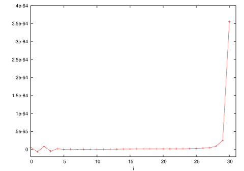
Figure 3: Effective FK vertex amplitude: all $j=30$, all $k=15$, all $i$ equal, satisfying $0\leq i\leq 2k$.

Figure 4: Effective FK vertex amplitude: all $j=30$, all $i=2k$, all $k$ equal, satisfying $0\leq k\leq j$.

For the FK model, we found that, for fixed $j$ and $k$, the amplitude is again maximized by the extreme value $i=2k$. See figure 3 for the case $j=30$ and $k=15$. While keeping $i$ at the dominant value $2k$, for fixed $j$, the amplitude is maximized by $k=1$, although $k=0$ dominates slightly for very small values of $j$. This $k$ dependence is illustrated in figure 4 for the case $j=30$.

Figure 5: Large $j$ behavior of the effective vertex amplitudes for the BC, EPR and FK models.

Spin foam quantization is similar in spirit to the discretized path integral approach to gravity. As such, the spin foam vertex amplitude is often compared to the gravitational path integral amplitude:

$$A_{v}(j)\sim\exp[iS_{R}],$$ (66)

where $S_{R}$ is the Regge action for gravity evaluated on a discrete geometry described by the spins $j$ in the large spin limit. For the BC vertex, this view has turned out to be overly simplistic. The relation predicted by careful asymptotic analysis is

$$A_{v}(j)\sim D(j)+\mu(j)[\exp(iS_{R})+\exp(-iS_{R})]+\cdots,$$ (67)

where $D(j)$ and $\mu(j)$ are non-oscillating functions decaying as $j^{-2}$ and $j^{-9/2}$ respectively, with $(\cdots)$ representing higher order terms. The dominant asymptotic $D(j)$, understood to be due to the contribution of degenerate geometries, masks the desired Regge action amplitude [BCE, FL, BS].

A natural question is whether the new vertices share the same asymptotic behavior. Numerical evaluation of the BC vertex is only sensitive to the dominant asymptotic contribution $D(j)$. The subdominant oscillating Regge action term would become important only if $D(j)$ is subtracted or if the vertex amplitude is averaged against another oscillatory function, in phase with one of the Regge action terms, as done in the graviton propagator calculations [R-prop, CLS]. While analytical asymptotics for the EPR and FK vertices are still missing, we can straightforwardly compare the numerical asymptotics of the dominant effective vertex amplitudes of all three models. This comparison is made in figure 5. For all models, the data shows no oscillations, which means that we are most likely seeing only the $D(j)$ asymptotic term. Note that the power laws shown in the figure will change if the edge or face amplitudes given in section 2 are modified by $j$-dependent factors. Such modifications can come, for instance, from different choices of exponent $k$ for factors of the form $(j_{f}+1)^{k}$, contributing to face amplitudes, as was considered in equation (3) of [CLS]. Different choices of this $k$ would correspond to different choices in the path integral analog of spin foams.

6.2 Wave packet propagation

As an immediate improvement over previous work, the algorithms presented in this paper allow us to show the effect of introducing a non-zero $\tau$ in (23) and to compare with the calculations of [MPR], which kept $\tau=0$, freezing all $j$-spins at the background value $j_{0}$. According to equation (25), the size of $\tau$ is inversely proportional to the parameter $\alpha$. Figure 6 compares the reference wave packet $\psi$ [cf. (24)] with several propagated wave packets $\phi$ (each with a different value of $\alpha$) depending on the single fixed $i$-spin. The wave packets have been normalized such that their absolute values squared sum to $1$. The wave packet with the largest value of $\alpha$ is essentially identical to the one obtained with all $j$-spins frozen at $j_{0}$. In that case, as shown previously in [MPR], the reference state $\psi$ resembles the propagated wave packet in shape and mean. Unfortunately, as the width of the gaussian factors associated to $j$-spins increases ($\alpha$ decreases), the propagated wave packet quickly departs from $\psi$ in both shape and mean. Notably, the mean shifts to a significantly higher value of $i$.

Figure 6: EPR 4-1 propagated ($\phi$) and reference ($\psi)$ wave packets, with $j_{0}=3$.

Figure 7: 9-1 propagated and reference wave packets for different models, with $j_{0}=3$.

Second, we can compare the wave packets propagated by the three different models in the 9-1 geometry. Figure 7 shows the reference wave packets $\psi$ [cf. (23)] and propagated wave packets $\phi$, depending on the fixed $j$-spin and for two choices of $\alpha$. These wave packets are also normalized. While he propagated wave packets seem to retain a roughly peaked shape, their mean and width mostly differ significantly from the reference wave packet. The only exception is the BC model at $\alpha=5$. However, this is likely a coincidence that does not appear for other choices of parameter values.

Lastly, we compare the wave packets propagated by the three different models in the 4-6 geometry. In general, the propagated wave packet will depend on the four fixed $j$-spins. Unfortunately, it is impractical to either compute or display functions on a $4$-dimensional domain. Thus, all calculations have been done with the four fixed $j$-spins set equal. Figure 8 shows the reference wave packet $\psi$ [cf. (23)] and propagated wave packets $\phi$, depending on the common value of the fixed $j$-spins for two choices of $\alpha$. These wave packets are again normalized. As is clearly seen from the figure, the propagated wave packets have in general very little similarity with the reference one. More pathological behavior is observed in the FK and BC models, the latter at $\alpha=1/2$, since none of these curves resemble a well formed gaussian wave packet. In all cases, the propagated wave packet has little in common with the reference one.

Figure 8: 4-6 propagated and reference wave packets for different models, with $j_{0}=4$.

7 Conclusion and outlook

We have presented three spin foam models in a unified framework: the standard Barrett-Crane (BC) model and two more recent proposals, the Engle-Pereira-Rovelli (EPR) and Freidel-Krasnov (FK) models. Their vertex amplitudes were simplified and explicitly evaluated using spin network recoupling techniques. Despite the different spin argument structure, we have proposed uniform methodologies for comparing the results of calculations of asymptotics of effective vertex amplitudes and of expectation values of specific spin foam observables among the different models. Building on the past work of Christensen & Egan, a fast numerical evaluation algorithm for the new vertex amplitudes, both in the absence and in the presence of (factored) boundary states, was developed and implemented. The run time complexity of these algorithms has been analyzed and shown to be orders of magnitude superior to more naive approaches. These algorithms were applied to the problems of extracting the asymptotic behavior of the new vertex amplitudes and to checking the behavior of propagated semiclassical wave packets.

The results presented in section 6.1 show that the dominant asymptotic behavior of the new vertex amplitudes is non-oscillatory and displays power-law decay very similar to the BC model, suggesting dominance of degenerate spin foams as for the BC model itself. The power law exponents are estimated in figure 5. It should be interesting to explore the asymptotics of these amplitudes with analytical techniques as well. It is likely that they will reveal structure similar to (67).

Although the boundary state proposed in section 2.3 is not ideal (see [RS] for a more realistic proposal), it has the advantage of belonging to the class of factored states, allowing efficient numerical computation with algorithms of section 5. Moreover, the proposed state can still be used to gauge the qualitative behavior of unfreezing the $j$-spins. Reference [MPR] had put forward the conjecture that semiclassical wave packets, propagated using the EPR dual vertex amplitude, approximate a certain reference gaussian shape, which was demonstrated under somewhat restrictive conditions. Application of the numerical algorithms described above allowed a broader investigation of this question. The class of factored boundary states encompasses the states used in the calculations that gave rise to this conjecture. The results of section 6 indicate that a generic factored boundary state does not exhibit good semiclassical behavior. It is likely that the presence of correlations between spins, which are not not captured by a factored state, improves the agreement between propagated and reference wave packets. However, until the use of more complicated states is possible, the evidence for the conjecture of Magliaro, Perini & Rovelli remains inconclusive.

These algorithms have also already been implemented and applied by other authors, as discussed in section 6.2. While, several wave packet propagation geometries have been examined, there are many other ones. Important questions remain: Is any one of them theoretically preferable to the others? What is the impact of directly using the unfactorable boundary state of [RS]? Another immediate possibility for further investigation is the computation of the graviton propagator matrix elements in the EPR and FK models.