Disk Dominated States of 4U 1957+11: Chandra, XMM, and RXTE Observations
of Ostensibly the Most Rapidly Spinning Galactic Black Hole

Abstract

We present simultaneous Chandra-High Energy Transmission Gratings (HETG) and Rossi X-ray Timing Explorer (RXTE) observations of a moderate flux ‘soft state’ of the black hole candidate 4U 1957+11. These spectra, having a minimally discernible hard X-ray excess, are an excellent test of modern disk atmosphere models that include the effects of black hole spin. The HETG data show, by modeling the broadband continuum and direct fitting of absorption edges, that the soft disk spectrum is only very mildly absorbed with ${\rm N_{H}}=1$–$2\times 10^{21}~{}{\rm cm}^{-2}$. These data additionally reveal $\lambda\lambda 13.449$ Ne IX absorption consistent with the warm/hot phase of the interstellar medium. The fitted disk model implies a highly inclined disk around a low mass black hole rapidly rotating with normalized spin $a^{*}\approx 1$. We show, however, that pure Schwarzschild black hole models describe the data extremely well, albeit with large disk atmosphere “color-correction” factors. Standard color-correction factors can be attained if one additionally incorporates mild Comptonization. We find that the Chandra observations do not uniquely determine spin, even with this otherwise extremely well-measured, nearly pure disk spectrum. Similarly, XMM-Newton/RXTE observations, taken only six weeks later, are equally unconstraining. This lack of constraint is partly driven by the unknown mass and unknown distance of 4U 1957+11; however, it is also driven by the limited bandpass of Chandra and XMM-Newton. We therefore present a series of 48 RXTE observations taken over the span of several years and at different brightness/hardness levels. These data prefer a spin of $a^{*}\approx 1$, even when including a mild Comptonization component; however, they also show evolution of the disk atmosphere color-correction factors. If the rapid spin models with standard atmosphere color-correction factors of ${\rm h_{d}}=1.7$ are to be believed, then the RXTE observations predict that 4U 1957+11 can range from a 3 ${\rm M_{\odot}}$ black hole at 10 kpc with $a^{*}\approx 0.83$ to a 16 ${\rm M_{\odot}}$ black hole at 22 kpc with $a^{*}\approx 1$, with the latter being statistically preferred at high formal significance.

1. Introduction

Despite having an X-ray brightness comparable to and occasionally exceeding that of LMC X-1 or LMC X-3, and despite also being one of the few persistent black hole candidates (BHC), 4U 1957+11 has received relatively little attention. Similar to LMC X-3 (see, e.g., Wilms et al., 2001), 4U 1957+11 is usually in a soft state that shows long term (hundreds of days) variations (Nowak & Wilms, 1999; Wijnands, Miller & van der Klis, 2002). Long term variations also have been seen in its optical lightcurve: modulation over its 9.33 hr orbital period has ranged from $\pm 10\%$ and sinusoidal (Thorstensen, 1987) to $\pm 30\%$ and complex (Hakala, Muhli & Dubus, 1999). Hakala, Muhli & Dubus (1999) interpret these changes in the optical lightcurve as evidence for an accretion disk with a large outer rim, possibly due to a warp, being nearly edge-on and partly occulted by the secondary. The lack of any X-ray evidence for binary orbital modulation (Nowak & Wilms, 1999; Wijnands, Miller & van der Klis, 2002) indicates that the orbital inclination cannot exceed $\approx 75^{\circ}$.

Observations with Ginga showed a soft spectrum that could be fit with a multi-temperature disk blackbody (diskbb; Mitsuda et al., 1984) plus a power law tail with photon index $\Gamma\approx 2$–3 (Yaqoob et al., 1993). The power-law component in those observations comprised up to 25% of the 1-18 keV flux. Later RXTE observations also were consistent with a disk blackbody model, but showed no evidence of either a hard component or any X-ray variability above background fluctuations (Nowak & Wilms, 1999). Wijnands, Miller & van der Klis (2002) conducted a series of Target of Opportunity observations designed to catch 4U 1957+11 at the high end of its count rate as determined by the All Sky Monitor (ASM) on-board of RXTE. They found that at its highest flux, 4U 1957+11 exhibited both a hard tail and mild X-ray variability.

For all of the above cited X-ray observations, the disk parameters had two attributes in common: the best fit inner disk temperatures were high (up to 1.7 keV), and the fitted normalizations were low ($\sim 10$). Nominally, the disk blackbody normalization corresponds to $(R_{\rm km}/D_{\rm 10})^{2}\cos\theta$, where $R_{\rm km}$ is the disk inner radius in km, $D_{\rm 10}$ is the source distance in units of 10 kpc, and $\theta$ is the inclination of the disk. In physical models, such large temperatures with such low normalizations normally can be achieved only by a combination of large distance, high inclination, low black hole mass, high accretion rate, and possibly rapid black hole spin. Disk temperatures increase as the 1/4 power of fractional Eddington luminosity, but decrease as the 1/4 power of black hole mass. Thus, lower mass serves to increase the temperature and decrease the normalization via decreasing $R_{\rm km}$. Large distances and high inclination also serve to reduce the normalization. (Again, the lack of X-ray eclipses limits $i\mathrel{\hbox to0.0pt{\raise 2.20013pt\hbox{$<$}\hss}{\lower 2.20013pt\hbox{$\sim$}}}75^{\circ}$.) Finally, rapid spin yields higher efficiency in the accretion disk (and thus higher temperatures), and a decreased inner disk radius.

As pointed out by a number of authors, however, the diskbb model is not a self-consistent description of a physical accretion disk (see, for example, Li et al., 2005; Davis et al., 2005; Davis, Done & Blaes, 2006). Several authors have developed more sophisticated models that incorporate a torque (or lack thereof) on the inner edge of the disk, atmospheric effects on the emerging disk radiation field, the effects of limb darkening and returning radiation (due to gravitational light bending), and the effects of black hole spin. Two of these models are the kerrbb model of Li et al. (2005) and the bhspec model of Davis et al. (2005). Using these models on soft-state BHC spectra with minimal hard tails, various claims have been made as to their ability to observationally constrain black hole spin (e.g., Shafee et al., 2006; Davis, Done & Blaes, 2006; McClintock et al., 2006; Middleton et al., 2006). Given the apparent dominance of a soft spectrum in 4U 1957+11, and the typical weakness of any hard tail, 4U 1957+11 becomes an excellent testbed for assessing the ability of these models to constrain physical parameters.

The outline of this paper is as follows. First, we describe the analysis procedure for the Chandra, XMM-Newton, and RXTE data (§2). We then discuss fits to the Chandra data with both phenomenological (i.e., diskbb) and more physically motivated (i.e., kerrbb) models (§3). We then discuss the XMM-Newton data, and specifically look at the absorption edge regions in both the Chandra gratings spectra and the XMM-Reflection Gratings Spectrometer (RGS) spectra (§3.2). We then discuss spectral fits to 48 observations from the RXTE archives (§4.1), and we consider the variability properties of these observations (§4.2). Finally, we present our conclusions and summary (§5).

2. Data Preparation

2.1. Chandra

4U 1957+11 was observed by Chandra on 2004 Sept. 7 (ObsID 4552) for 67 ksec (two binary orbital periods). The High Energy Transmission Gratings (HETG; Canizares et al., 2005) were inserted. The HETG is comprised of the High Energy Gratings (HEG), with coverage from $\approx 0.7$–8 keV, and the Medium Energy Gratings (MEG), with coverage from $\approx 0.4$–8 keV. The data readout mode was Timed Exposure-Faint. To minimize pileup in the gratings spectra, a 1/2 subarray was applied to the CCDs, and the aimpoint of the gratings was placed closer to the CCD readout. This configuration reduces the readout time to 1.741 sec, without any loss of the dispersed spectrum.

We used CIAO v3.3 and CALDB v3.2.0 to extract the data and create the spectral response files. The location of the center of the $0^{\rm th}$ order image was determined using the findzo.sl routine, which provides $\approx 0.1$ pixel ($\approx 0.001$ Å, for MEG) accuracy. The data were reprocessed with pixel randomization turned off, but pha randomization left on. We applied the standard grade and bad pixel file filters, but we did not destreak the data. (We find that for sources as bright as 4U 1957+11, destreaking the data can remove real photon events, while order sorting is already very efficient at removing streak events.)

Although our instrumental set up was designed to minimize pileup, it is still present in both the MEG and HEG spectra. Pileup serves to reduce the peak of the MEG spectra, which occurs near 2 keV, by approximately 13%, while it reduces the peak of the HEG spectra by approximately 3%. In the Appendix we describe how we incorporate the effects of pileup in our model fits to the Chandra data.

All analyses, figures, and tables presented in this work were produced using the Interactive Spectral Interpretation System (ISIS; Houck & Denicola 2000). (Note: all ‘unfolded spectra’ shown in the figures were generated using the model-independent definition provided by ISIS; see Nowak et al. 2005 for further details.) For our $\chi^{2}$-minimization fits to Chandra data, we take the statistical variance to be the predicted model counts, as opposed to the observed data counts. (Choosing the former aids in our Bayesian line searchs; see §3.2.) Additionally, we evaluated the model for each individual gratings arm, but calculated the fit statistic using the ISIS combine_datasets function to add the data from the gratings arms. The Chandra data show very uniform count rates and spectral colors over the course of the observation, therefore throughout we use data from the entire 67 ksec observation.

2.2. XMM-Newton

4U 1957+11 was observed by XMM-Newton on 2004 Oct. 16 (ObsID 206320101) for 45 ksec. XMM-Newton carries three different instruments, the European Photon Imaging Cameras (EPIC; Strüder et al., 2001; Turner et al., 2001) the Reflection Grating Spectrometers (RGS; den Herder et al., 2001), and the Optical Monitor (OM; Mason et al., 2001). The OM was not used in this analysis.

The EPIC instruments consist of 3 CCD cameras, MOS-1, MOS-2, and pn, each of which provides imaging, spectral and timing data. The pn and MOS-1 cameras were run in timing mode which provides high time resolution event information by sacrificing 1-dimension in positional information. The MOS-2 camera was run in full-frame mode. The EPIC instruments provide good spectral resolution ($\Delta E$$=$50–200 eV FWHM) over the 0.3–12.0 keV range. There are two RGS detectors onboard XMM-Newton which provide high-resolution spectra ($\lambda/\Delta\lambda$$=$100–500 FWHM) over the 5–38 Å  range. The grating spectra are imaged onto CCD cameras similar to the EPIC-MOS cameras which allows for order sorting of the high-resolution spectra.

The XMM-Newton data were reduced using SAS version 7.0. Standard filters were applied to all XMM-Newton data. The EPIC-pn data were reduced using the procedure epchain. We reduced the EPIC-MOS data using emchain. Source and background spectra for the pn and MOS-1 data were extracted using filters in the one spatial coordinate, RAWX. Response files were created using the SAS tools rmfgen and arfgen. The MOS-2 data were found to be considerably piled up and were therefore not used in this analysis.

The RGS data were reduced using rgsproc, which produced standard first order source and background spectra and response files for both detectors.

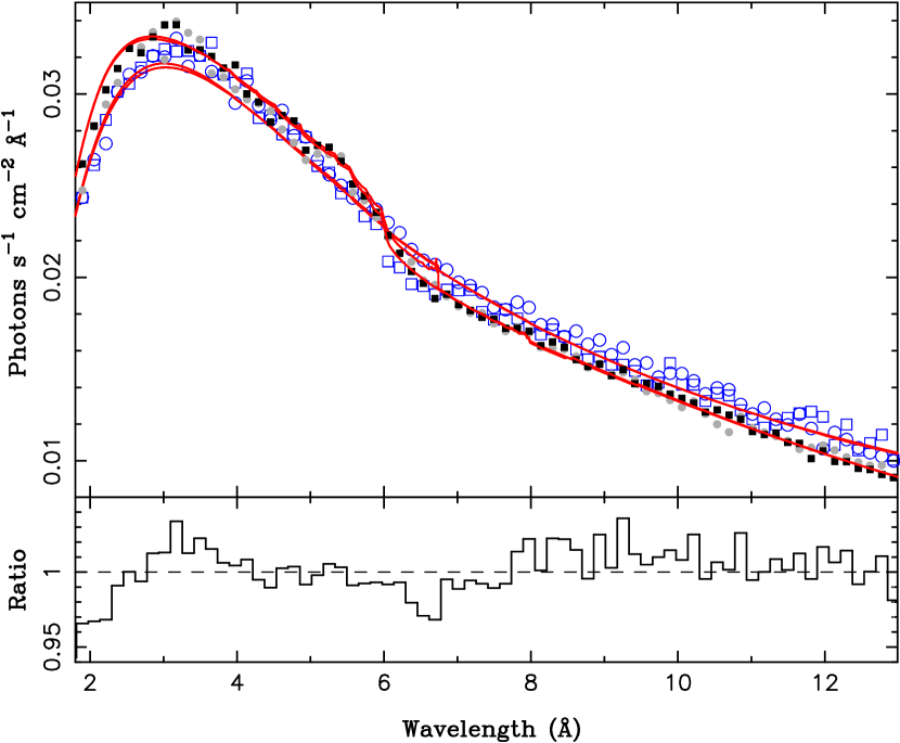
Figure 1.— Fits to the summed HEG (hollow points) and MEG (solid points) data in the 1.8–13 Årange. The neutral column was fixed to be the same for all data sets, but pileup correction was treated on an individual detector basis, and the HEG diskbb parameters were allowed to differ from the MEG diskbb parameters.

2.3. RXTE

During the past ten years, RXTE has observed 4U 1957+11 numerous times. The first of these observations was presented in Nowak & Wilms (1999). A series of observations, specifically triggered to observe high flux states, were presented in Wijnands, Miller & van der Klis (2002). One RXTE observation was scheduled to occur simultaneously with the Chandra observation (PI: Nowak), while another was scheduled to occur simultaneously with the XMM-Newton observation (PI: Homan). The remaining observations come from different monitoring campaigns, conducted by various groups. We obtained all of these data from the archives – 108 ObsIDs, 4 of which we exclude as they occurred during a brief period when RXTE experienced poor attitude control. We combine ObsIDs wherein the observations were performed within a few days of one another and color-intensity diagrams indicate little or no evolution of the source spectra, yielding 48 spectra.

The data were prepared with the tools from the HEASOFT v6.0 package. We used standard filtering criteria for data from the Proportional Counter Array (PCA). Specifically, we excluded data from within 30 minutes of South Atlantic Anomaly (SAA) passage, from whenever the target elevation above the limb of the earth was less than $10^{\circ}$, and from whenever the electron ratio (a measure of the charged particle background) was greater than 0.15. Owing to the very modest flux of 4U 1957+11, we used the background models appropriate to faint data. We also extracted data from the High Energy X-ray Timing Experiment (HEXTE), but as 4U 1957+11 is both faint and very soft, none of these data were of sufficient quality to use for further analysis.

We applied 0.5% systematic errors to all PCA channels, added in quadrature to the errors calculated from the data count rate. For all PCA fits, we grouped the data, starting at $\geq 3$ keV, with the criteria that the signal-to-noise (after background subtraction, but excluding systematic errors) in each bin had to be $\geq 4.5$. We then only considered data for which the lower boundary of the energy bin was $\geq 3$ keV, and the upper boundary of the energy bin was $\leq 18$ keV. This last criterion yielded upper cutoffs ranging from 12–18 keV.

3. Spectra Viewed with Chandra and XMM-Newton

3.1. Broadband Spectra

Our main goals in modeling the Chandra data are to describe the broad band continuum, accurately fit the edge structure due to interstellar and/or local-system absorption, and to search for narrow emission and absorption line features. To accurately describe the absorption due to the interstellar medium, we use tbnew, an updated version of the absorption model of Wilms, Allen & McCray (2000), which models the Fe $L_{2}$ and $L_{3}$ edges, and includes narrow resonance line structure in the Ne and O edges, as have been observed at high spectral resolution with Chandra-HETG (Juett, Schulz & Chakrabarty, 2004; Juett et al., 2006, abundances and depletion factors used here have been set to be consistent with these previous studies, i.e., they take on the default parameter values of the model, with the exception of the Fe abundance parameter being set to 0.647, and the Fe and O depletion parameters both being set to 1).

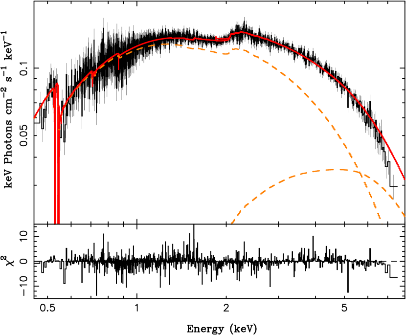
Figure 2.— A disk plus Comptonization model (see text) fit to the combined MEG data. Dashed lines show the individual model components.

We began by jointly modeling both the HEG and the MEG spectra; however, as seen in Fig. 1, we find systematic differences (up to $\approx 5$%, which is less than the statistical noise level shown in the figure) between the gratings arms, especially at low energies, which cannot be accounted for via the pileup modeling. Specifically, the HEG spectra show a greater soft excess, such that fits to solely those data in the 0.7–8 keV range with an absorbed diskbb model yield no absorption, contrary to the edge structure detected by MEG below 0.7 keV. Given the disagreements with MEG, the lack of a fittable column in HEG, the lack of apparent lines in the 1–8 keV region (see below), and the fact that the MEG allows us to model line and edge structure in the 0.5–1 keV region, we shall only consider MEG data.

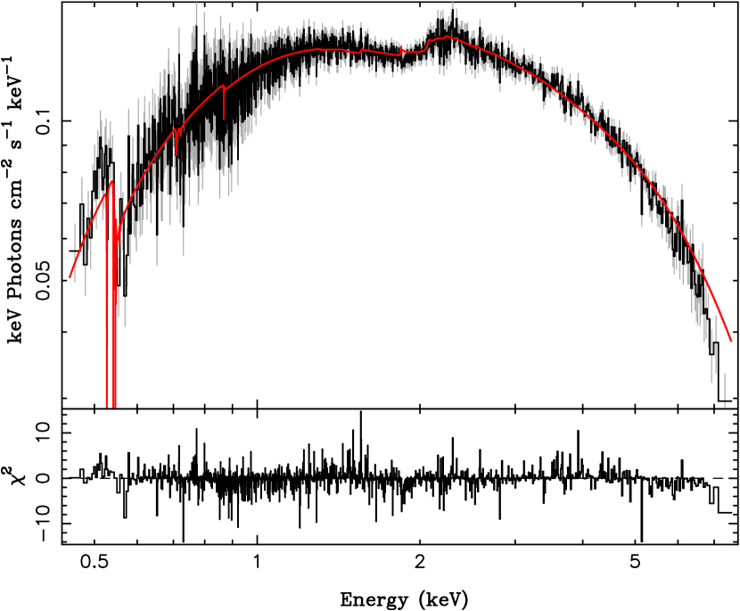
Figure 3.— Left: The kerrbb model, with $a^{*}\approx 1$, fit to the combined MEG data. System distance, inclination, and mass were fixed (see text), but spectral hardening factor and black hole spin were left free. Right: same data and model as on the left, except that now the black hole spin is fixed to $a^{*}=0$.

Systematic disagreements were also found between the simultaneous Chandra and RXTE data. The RXTE data were slightly softer in the regions of overlap ($\approx 4$–7 keV), and owing to the very large effective area of RXTE, we found that the latter instrument dominated any joint fits. The two instruments fit qualitatively similar models with comparable parameters; however, no joint model, even when applying systematic errors to the PCA data, produced formally acceptable fits. The differences between the instruments are likely attributable to calibration uncertainties for both, and therefore we chose to analyze the Chandra and RXTE data independently.

For our subsequent broadband spectral fits to the MEG data, we grouped the $\pm 1^{\rm st}$ orders to a combined signal-to-noise of $\geq 6$ and a minimum of two wavelength channels (i.e., 0.01 Å) per bin. We then fit the data in the 0.45–7.75 keV region. Results are presented in Table 1. Overall, the spectra are well-described by a very mildly absorbed (${\rm N_{H}}\approx 1$–$1.2\times 10^{21}~{}{\rm cm^{-2}}$) diskbb spectrum, with a fairly high temperature (${\rm kT_{in}}=1.75$ keV), but low normalization (${\rm A_{dbb}}=7.2$), with little need for additional features such as a narrow or broad Fe K$\alpha$ line (cf. §3.2). Formally, if we add a line with fixed energy and width of 6.4 keV and 0.5 keV, respectively, the 90% confidence upper limit the line flux is $7\times 10^{-5}$ ph cm^-2 s^-1.

The low disk model normalization could correspond to a combination of low black hole mass, high inclination, and large distance. The fitted temperature is on the high side for a ‘soft state’ BHC. Fits to soft states of LMC X-1 and LMC X-3, for example, have consistently found ${\rm kT_{in}}\mathrel{\hbox to0.0pt{\raise 2.20013pt\hbox{$<$}\hss}{\lower 2.20013pt\hbox{$\sim$}}}1.25$ keV (Nowak et al., 2001; Wilms et al., 2001; Davis, Done & Blaes, 2006), while our own fits to RXTE and ASCA data of 4U 1957+11 have found ${\rm kT_{in}}\mathrel{\hbox to0.0pt{\raise 2.20013pt\hbox{$<$}\hss}{\lower 2.20013pt\hbox{$\sim$}}}1.6$ keV. Such a high temperature might be taken as a hallmark of some combination of high accretion rate, low black hole mass, and/or high black hole spin. Another possibility is the presence of a Comptonizing corona, serving to harden any disk spectrum.

To show, at least qualitatively, how the presence of a corona would affect our disk fit parameters, we added the comptt Comptonization model (Titarchuk, 1994), to the diskbb model, even though the disk fit residuals do not indicate the necessity of an extra component. Given the quality of the simple disk fit, we chose to reduce the number of free parameters by tying the temperature of the seed photons input to the corona to the temperature of the disk inner edge. Furthermore, we froze the temperature of the corona itself to 50 keV. The additional fit parameters were then the coronal plasma optical depth, $\tau_{\rm p}$ (with its lower limit set to 0.01), and the normalization of the coronal spectrum. Results of this fit are shown in Fig. 2 and are presented in Table 1.

Table 1Broadband Fits to MEG Data

${\rm N_{H}}$	${\rm A_{dbb}}$	${\rm kT_{in}}$	$a^{*}$	${\rm\dot{M}}$	${\rm h_{d}}$	${\rm P_{frac}}$	${\rm A_{comptt}}$	$\tau_{\rm p}$	${\rm kT_{0}}$	$\chi^{2}/$dof
$(10^{21}~{}{\rm cm^{-2}})$		(keV)		($10^{17}~{}{\rm g~{}s^{-1}}$)			($10^{-2}$)		(keV)
$1.04^{+0.04}_{-0.03}$	$7.18^{+0.18}_{-0.11}$	$1.74^{+0.02}_{-0.01}$	$\cdots$	$\cdots$	$\cdots$	$0.128^{+0.007}_{-0.008}$	$\cdots$	$\cdots$	$\cdots$	1861/1588
$1.06^{+0.02}_{-0.04}$	$17.87^{+1.45}_{-0.03}$	$1.25^{+0.03}_{-0.03}$	$\cdots$	$\cdots$	$\cdots$	$0.124^{+0.002}_{-0.008}$	$0.147^{+0.001}_{-0.002}$	$0.01^{+0.01}_{-0.00}$	50	1850/1586
$1.02^{+0.02}_{-0.02}$	$\cdots$	$\cdots$	$0.9999^{+0.0000}_{-0.0002}$	$0.548^{+0.001}_{-0.002}$	$1.220^{+0.002}_{-0.003}$	$0.132^{+0.002}_{-0.007}$	$\cdots$	$\cdots$	$\cdots$	1862/1587
$1.07^{+0.04}_{-0.05}$	$\cdots$	$\cdots$	$0.952^{+0.002}_{-0.003}$	$1.40^{+0.02}_{-0.03}$	1.7	$0.130^{+0.007}_{-0.008}$	$\cdots$	$\cdots$	$\cdots$	1933/1587
$1.13^{+0.04}_{-0.04}$	$\cdots$	$\cdots$	0	$7.26^{+0.04}_{-0.04}$	$3.41^{+0.03}_{-0.02}$	$0.126^{+0.007}_{-0.008}$	$\cdots$	$\cdots$	$\cdots$	1892/1588

Note. — The $\chi^{2}$ statistic was calculated by using the predicted model counts as the variance. Error bars are 90% confidence values ($\Delta\chi^{2}=2.7$) for one interesting parameter. Parameters in italics were held frozen at that value. diskbb normalization, ${\rm A_{dbb}}$, is ${\rm[(R_{in}/1\,km)(D/10\,kpc)]^{2}\cos\theta}$. For further details of the fits, see the text.

Although the improvement to the fit is only very mild ($\Delta\chi^{2}=11$), we see that the temperature of the diskbb component drops to 1.25 keV, while its normalization constant increases by more than a factor of 2. The comptt component now comprises $\approx 30\%$ of the implied bolometric flux. Furthermore, at energies $\mathrel{\hbox to0.0pt{\raise 2.20013pt\hbox{$>$}\hss}{\lower 2.20013pt\hbox{$\sim$}}}3$ keV it is consistent with a $\Gamma\approx 2$ photon index power law; however, this latter fact is tempered by the limited bandpass of Chandra at these energies. In a “physical interpretation” of these results, we see that a very weak, mild corona can qualitatively replace the need for an unusually hot, low normalization disk.

As an alternative for explaining the high disk temperature, we can consider spin of the black hole. Although the simple, two parameter diskbb model does an extremely good job of modeling the MEG spectra, it has a number of shortcomings from a theoretical perspective (see Davis, Done & Blaes, 2006). Its temperature profile is too peaked at the inner edge, its implied radiative efficiency does not match realistic expectations, it incorporates no atmospheric physics, and it includes no (special or general) relativistic effects. In response to these model shortcomings, several authors have developed more sophisticated disk models, specifically the kerrbb model of Li et al. (2005) and the bhspec model of Davis, Done & Blaes (2006). Here we consider the former model.

The kerrbb model increases the number of disk parameters from two to seven, and it allows other effects to be included, such as limb darkening and returning radiation to the disk from gravitational light bending (both turned on for fits described in this paper). The fit parameters are the mass, spin ($a^{*}$), and distance to the black hole, the mass accretion rate through the disk (${\rm\dot{M}}$), the inclination of the accretion disk to the line of sight, a torque applied to the inner edge of the disk (here set to zero), and a spectral hardening factor (${\rm h_{d}}$). The latter is to absorb uncertainties of the disk atmospheric physics, and represents the ratio of the disk’s color temperature to its effective temperature. Preferred values have been ${\rm h_{d}}\sim 1.7$ (Li et al., 2005; Shafee et al., 2006; McClintock et al., 2006), while other models (e.g., bhspec) attempt to calculate color corrections from first principles (Davis, Done & Blaes, 2006).

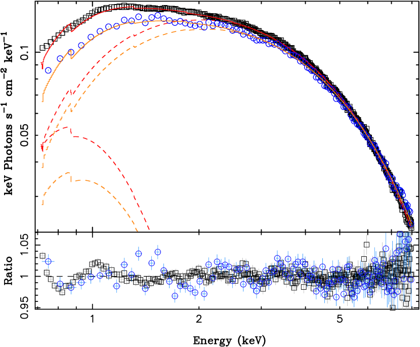
Figure 4.— Flux-corrected XMM-Newton EPIC-pn (squares) and -MOS-1 spectra (circles), fit with independent absorbed diskbb+diskbb models in the 0.7–8 keV range. Dashed lines show the individual absorbed disk components for the fit. 0.05% systematic errors were added to the pn data, while 1% systematic errors were added to the MOS data.

To reduce the fit complexity of the kerrbb model to match the two parameters of the diskbb model, one typically invokes knowledge obtained from other observations (i.e., for system mass, distance, and inclination) and from theoretical expectations (i.e., for inner edge torque and ${\rm h_{d}}$). The former is lacking for 4U 1957+11. Here we fix the inclination to $75^{\circ}$, to be consistent with the both the optical and X-ray lightcurve behavior (Hakala, Muhli & Dubus, 1999; Nowak & Wilms, 1999). Furthermore, we fix the mass to 3 ${\rm M_{\odot}}$ and the distance to 10 kpc. We discuss these choices further in §4.1 and §5, but here we note that these latter choices allow the closest possible distance to 4U 1957+11, while still maintaining a minimum inferred bolometric luminosity of $>3\%\,{\rm L_{Edd}}$. Finally, we set the torque parameter to 0, as its value is essentially subsumed by degeneracies with the fitted mass accretion rate (Li et al., 2005; Shafee et al., 2006).

Allowing the spectral hardening factor, ${\rm h_{d}}$ to remain free, we obtain a kerrbb fit to the MEG spectra that is of comparable quality to the simple diskbb fit. We note, however, that the fitted value of ${\rm h_{d}}=1.22$ is smaller than the commonly preferred value of 1.7 (see Done & Davis, 2008), and that the black hole spin is found to be near unity ($a^{*}=0.9999$). Again, the latter is being driven by the fact that the fitted diskbb temperature is itself rather high for a soft state BHC system. Freezing ${\rm h_{d}}=1.7$, we obtain a slightly worse, but still reasonable, fit ($\Delta\chi^{2}=71$), with a large inferred black hole spin ($a^{*}=0.95$). If instead we freeze the spin $a^{*}=0$, but allow the spectral hardening factor to be free, we obtain a $\chi^{2}$ intermediate to those of the previous two fits ($\Delta\chi^{2}=30$ from the best kerrbb fit), but with ${\rm h_{d}}=3.41$. This rather large value is well-outside the normal range of variation (${\rm h_{d}}=$1.4–1.8; Done & Davis 2008). As shown in Fig. 3, however, these fits are virtually indistinguishable from one another.

We next consider broadband fits to XMM-Newton data. These XMM-Newton observations occured only 6 weeks after the Chandra observations, with apparently little source variation as measured by the RXTE-ASM in the intervening period. As we further discuss in §4, the XMM-Newton spectra showed a flux and spectral hardness comparable to the Chandra spectra. Thus, we expect the XMM-Newton spectra to be qualitatively and quantitatively similar to the Chandra spectra. We have found that in practice, the XMM-Newton spectra are somewhat difficult to fit over their entire spectral range, and furthermore, the EPIC-pn and -MOS data do not completely agree with one another. For a variety of models that we tried, strong, sharply peaked residuals occurred for both detectors near 0.5 keV (the O K edge), although these residuals were most pronounced in the pn data. Above 8 keV, the two detectors also show (different from each other, and from RXTE) spectral deviations from simple models. Accordingly, we only consider data in the 0.7–8 keV range. Additionally, we add uniform 0.5% (pn) and 1% (MOS) systematic errors to each spectrum. (These levels were required to obtain reduced $\chi^{2}\approx 1$–2 with ‘simple’ spectral models.)

The only simple models that we found to adequately describe the data required an additional spectral component below 2 keV, which here we model as a second diskbb component with ${\rm kT_{in}}\approx 0.3$ keV and ${\rm A_{dbb}}\approx 1300$ (MOS) and $\approx 2600$ (pn). The required ${\rm N_{h}}\approx 3\times 10^{21}\,{\rm cm^{-2}}$ for both detectors was somewhat larger than that found for MEG. The dominant disk component, primarily required to fit the 2-8 keV spectra, had comparable parameters to the diskbb fit to the MEG data; namely, ${\rm A_{dbb}}\approx 8$ and ${\rm kT_{in}}\approx 1.6$ keV.

Significant residuals clearly remain in the 0.7–2 keV range for both the pn and MOS data, and the pn and MOS spectra quantitatively disagree with each other. Given the fact that the MEG spectra, as well as prior ASCA spectra (Nowak & Wilms, 1999) were well described with a simple absorbed diskbb model, with lower ${\rm N_{H}}$, we are inclined to ascribe a large fraction of the additional required $\approx 0.3$ keV disk component and the low energy residuals to systematic errors in the XMM-Newton calibration.

With the above caveats in mind, the XMM-Newton data, however, confirm that in the 2–8 keV range, the characteristic disk temperature for 4U 1957+11 is indeed rather large. Furthermore, the XMM-Newton spectra show no evidence for any narrow, or moderately broad, Fe K$\alpha$ line. Similar to the Chandra data, adding a 6.4 keV line with 0.5 keV width (both fixed) yields a 90% confidence upper limit to the line flux of $6\times 10^{-5}$ ph cm^-2 s^-1.

Table 2Absorption Lines Fit to MEG and RGS Data

Line	$\lambda$	Eq. Width
	(Å)	(mÅ)
Neix	$13.449^{+0.005}_{-0.005}$	$-7.2^{+2.8}_{-2.2}$
Neiii	14.508	$-6.0^{+3.3}_{-3.0}$
Neii	$14.611^{+0.005}_{-0.005}$	$-7.5^{+4.8}_{-3.1}$
Oviii K$\beta$	18.629	$-9.9^{+9.9}_{-9.0}$
Oviii K$\alpha$	18.967	$-21^{+11}_{-10}$
Ovii	21.602	$-18^{+18}_{-16}$
?	$21.80^{+0.04}_{-0.04}$	$-71^{+36}_{-43}$
Oii	23.375	$-15^{+15}_{-18}$
Oviii K$\beta$	18.629	$0^{+0}_{-14}$
Oviii K$\alpha$	18.967	$-28^{+15}_{-14}$
Ovii	21.602	$-36^{+29}_{-24}$
?	$21.80^{+0.02}_{-0.02}$	$-67^{+44}_{-36}$
Oii	23.375	$-11^{+11}_{-29}$
Oviii K$\beta$	$18.62^{+0.03}_{-0.03}$	$-8.5^{+8.5}_{-5.4}$
Oviii K$\alpha$	$18.96^{+0.02}_{-0.02}$	$-14^{+14}_{-5}$
Ovii	$21.59^{+0.03}_{-0.03}$	$-19^{+19}_{-11}$
?	$21.83^{+0.03}_{-0.03}$	$-23^{+11}_{-11}$
Oii	23.375	$-29^{+11}_{-11}$

Note. — Italicized parameters were held fixed. Errors are 90% confidence level.

3.2. Edge and line fits

We have employed a variety of techniques to search for lines in the 4U 1957+11 data, ranging from direct fits of narrow components at known line locations to a “blind search” using a Bayesian Blocks technique. The latter involves fitting a continuum model to the binned data, using the predicted model counts as the statistical variance in the fits, and then unbinning the data and comparing the likelihood of the observed counts to the predicted counts. (For a successful application of this technique to Chandra-HETG data of the low luminosity active galactic nuclei, M81*, see Young et al. 2007.) No candidate features that appear to be local to the 4U 1957+11 system were found. This is in contrast to, for example, Chandra observations of GROJ1655$-$40, which at a similar source luminosity in a spectrally soft, disk-dominated state showed very strong absorption features associated with the disk atmosphere (Miller et al., 2006). Comparable equivalent width features would have been very easily detected in our observation of 4U 1957+11. We note, however, that GROJ1655$-$40 itself has not always shown disk atmosphere absorption features. Two weeks prior to the observation described by Miller et al. (2006), despite the source being only slightly fainter while also being in a soft, disk-dominated state, Chandra-HETG observations revealed no narrow emission or absorption lines (Miller et al., 2006, 2008). The ‘duty cycle’ with which such lines are prominent in disk-dominated BHC spectra comparable to the spectra of both GROJ1655$-$40 and 4U 1957+11, remains an open observational question.

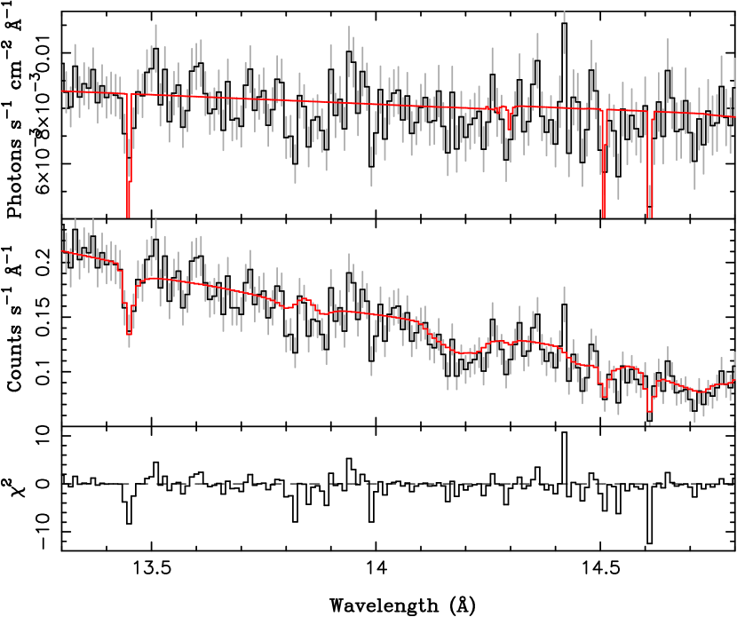
Figure 5.— Flux corrected spectra (top panel) and count rate per angstrom (middle panel) for the combined MEG $\pm 1^{\rm st}$ order spectra, with an absorbed diskbb model fit in the 13–15 Å region (see text). The top and middle panels show the data fit with the Ne II, Ne III, and Ne IX lines, while the residuals show a fit without the lines.

On the other hand, the above Bayesian Blocks procedure yielded a few candidate features in the Chandra data that are likely attributable to absorption by the Interstellar Medium (ISM). The strongest such feature is the absorption line at 13.44 Å. This feature is consistent with Ne IX absorption from the hot phase of the interstellar medium (Juett et al., 2006). Accordingly, we also simultaneously fit expected features from Ne II and Ne III absorption at 14.61 Å and 14.51 Å, respectively.

We again choose an absorbed disk model, albeit with the pileup fraction fixed to the values from our broad-band models, and only consider the 13–15 Å region. We group the spectrum to a minimum signal-to-noise of 5 in each bin, and we let the equivalent widths and wavelengths of the Ne IX and Ne II lines be free parameters while fixing the wavelength of the Ne III absorption to 14.508 Å. Results from this fit are presented in Fig. 5 and Table 2. The fitted wavelengths of the Ne IX and Ne II lines agree well with the MEG studies of Juett et al. (2006), although we find the Ne IX line wavelength to be redshifted by 0.005 Å (i.e., 111 km s^-1). Our fits, however, are within 0.002 Å of the theoretical value of 14.447 Å.

Formally, the fit improves with addition of any of the three Ne lines, although the Ne III region residual is far from the strongest in the overall spectrum. The Ne IX and Ne II absorption lines are more clearly detected. Their equivalent widths are near the mid-level to higher end of the sample discussed by Juett et al. (2006). As we discuss in greater detail elsewhere (Yao et al., 2008), the 4U 1957+11 Ne IX equivalent width is consistent with the source’s probable location outside the disk of the Galaxy. Specifically, presuming that 4U 1957+11 is greater than 5 kpc distant, and choosing a model where the hot phase of the ISM lies in layers predominantly outside the galactic plane, the equivalent width of the Ne IX line in 4U 1957+11 is consistent with the equivalent width of the same feature observed in the Active Galactic Nuclei Mkn 421, appropriately scaled for that sightline through our Galaxy. Therefore it is likely that 4U 1957+11 is sampling a large fraction of the hot phase interstellar gas that lies within and directly outside the galactic plane (Yao & Wang, 2007).

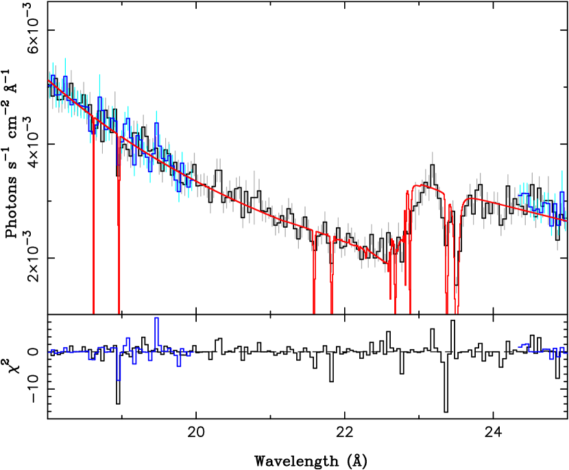
Figure 6.— Flux corrected RGS spectra in the 18–25 Å (RGS1) and 18-19.9 Å (RGS2) range, fit with a model consisting of interstellar absorption, a phenomenological continuum model (a broken power law plus multicolor blackbody), and various absorption lines (see Table 2). The residuals show the fit without the lines.

Consistent with this picture, both the RGS and MEG spectra show evidence of longer wavelength features that we also associate with absorption by the interstellar medium (Table 2; see also Yao et al. 2008). For the RGS data, we grouped both the RGS1 (fit between 18–25 Å) and RGS2 (fit between 18–19.9 Å) data to have a signal-to-noise of 5 and a minimum of four channels per bin. The MEG data were grouped to either 16 channels per bin, or 32 channels per bin. The MEG data were fit with an absorbed disk blackbody, while the RGS data required additional continuum structure (which we modeled here with a broken power-law). For all these model fits we added absorption lines expected from the warm and hot phases of the interstellar medium. The O II line from the warm phase of the ISM (not included in the tbnew model; Juett, Schulz & Chakrabarty 2004) is clearly detected by the RGS data, and consistent limits are found with the MEG data.

The hot phase of the ISM is detected with both the RGS and MEG via O VIII K$\alpha$ absorption (18.96 Å) measurements. The presence of O VIII K$\beta$ (18.63 Å) is not strictly required, but the limits on its equivalent width are consistent with the measured K$\alpha$ line (Yao et al., 2008). In addition to O VIII, we also find evidence for O VII K$\alpha$ absorption. Interestingly, an even stronger feature is detected at 21.8 Å. We have no good identification for this feature (it is 3000 ${\rm km~{}s^{-1}}$ redshifted from O VII). Its equivalent width might change between the MEG and RGS observations, and therefore it could be a candidate for a line intrinsic to the source.

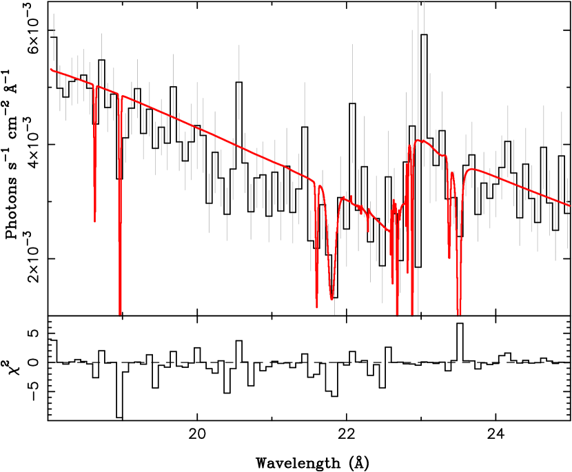
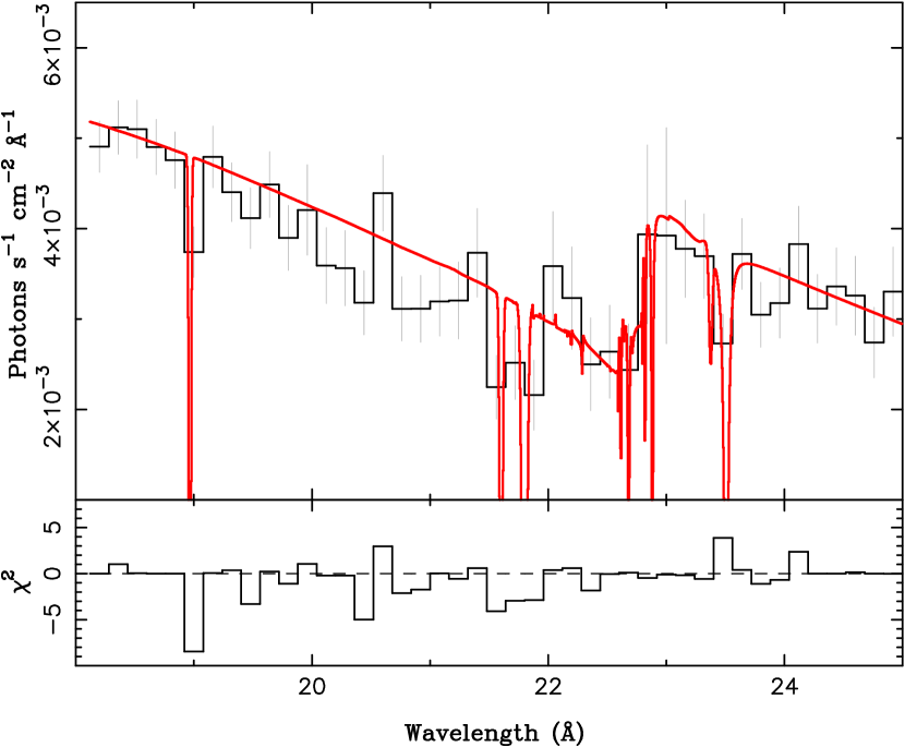
Figure 7.— Flux corrected MEG spectra in the 18–25 Å range, fit with a model consisting of interstellar absorption, a multicolor blackbody, and various absorption lines (see Table 2). The residuals show the fit without the lines. The top panel shows the spectra grouped to 16 channels per bin, while the bottom panel shows the spectra grouped to 32 channels per bin.

It is interesting to note that for the 18–25 Å fits discussed above, we find that the implied neutral column is somewhat larger than that found with the broadband fits. Specifically, we find $N_{H}=1.9\pm 0.2$, $1.8\pm 0.5$, and $2.0\pm 0.2$ $\times 10^{21}~{}{\rm cm^{-2}}$ for the RGS and MEG (16 channels per bin, 32 channels per bin) data. These values are primarily driven by the O edge region of the fits, although we have found for our broadband fits that merely changing the O abundance is insufficient to bring their fitted neutral columns into agreement with the 18–25 Å fits. It is possible that an additional very low energy component added to the broad band fits might allow for a larger column that is consistent with these narrow band fits.

4. RXTE Observations

In the previous sections we have shown that the 4U 1957+11 spectrum is consistent with a disk having a high peak temperature. One could reduce the need for this large peak temperature by including a hard component, e.g., a Comptonization spectrum; however, this added component only becomes dominant at photon energies above the bandpasses of Chandra and XMM-Newton. Thus, to distinguish between the possibilities of high black hole spin or an additional hard spectral component leading to the high fitted temperatures, we turn toward the RXTE data, which can provide spectral information up to $\approx 20$ keV for 4U 1957+11.

Table 3(diskbb+gaussian)+powerlaw, or +comptt Fits to Selected RXTE Data

ID	MJD	${\rm A_{dbb}}$	${\rm T_{in}}$	${\rm A_{pl}}$	$\Gamma$	${\rm A_{comptt}}$	$\tau_{\rm p}$	${\rm A_{line}}$	$\sigma_{\rm line}$	$\chi^{2}/$dof
			(keV)	$(10^{-2})$		$(10^{-5})$		$(10^{-4})$	(keV)
40044-01-02-01	51271	$5.05^{+0.47}_{-0.47}$	$1.801^{+0.022}_{-0.019}$	$28.54^{+5.45}_{-4.99}$	$2.13^{+0.07}_{-0.07}$	$\cdots$	$\cdots$	$3.9^{+1.7}_{-1.7}$	$0.0^{+0.6}_{-0.0}$	48.9/28
		$24.98^{+0.02}_{-3.03}$	$1.226^{+0.001}_{-0.001}$	$\cdots$	$\cdots$	$249.8^{+0.8}_{-0.8}$	$0.22^{+0.00}_{-0.00}$	$2.4^{+1.2}_{-1.2}$	$0.0^{+0.8}_{-0.0}$	25.1/28
70054-01-11-00	52656	$12.40^{+0.05}_{-0.04}$	$1.313^{+0.001}_{-0.001}$	$0.00^{+0.45}_{-0.00}$	$3.00^{+0.00}_{-2.00}$	$\cdots$	$\cdots$	$3.9^{+0.5}_{-0.5}$	$0.8^{+0.2}_{-0.1}$	16.7/18
		$12.52^{+0.04}_{-0.08}$	$1.311^{+0.001}_{-0.001}$	$\cdots$	$\cdots$	$0.0^{+1.1}_{-0.0}$	$0.53^{+4.47}_{-0.52}$	$4.2^{+0.5}_{-0.9}$	$0.8^{+0.2}_{-0.2}$	16.4/18
90123-01-03	53255	$11.49^{+0.24}_{-0.32}$	$1.554^{+0.008}_{-0.007}$	$0.71^{+4.31}_{-0.70}$	$2.38^{+0.62}_{-1.38}$	$\cdots$	$\cdots$	$4.6^{+1.9}_{-1.5}$	$0.5^{+0.3}_{-0.4}$	25.7/26
		$12.10^{+0.03}_{-0.72}$	$1.533^{+0.026}_{-0.013}$	$\cdots$	$\cdots$	$5.6^{+0.4}_{-4.8}$	$0.01^{+4.99}_{-0.00}$	$4.9^{+1.8}_{-0.8}$	$0.5^{+0.3}_{-0.2}$	25.3/26
90063-01-01	53294	$11.48^{+0.29}_{-0.30}$	$1.552^{+0.007}_{-0.006}$	$1.61^{+0.02}_{-1.60}$	$2.60^{+0.40}_{-1.60}$	$\cdots$	$\cdots$	$5.0^{+1.8}_{-1.6}$	$0.6^{+0.2}_{-0.3}$	19.0/26
		$12.24^{+0.42}_{-0.78}$	$1.529^{+0.029}_{-0.015}$	$\cdots$	$\cdots$	$6.4^{+0.8}_{-5.1}$	$0.01^{+4.99}_{-0.00}$	$5.2^{+1.6}_{-1.7}$	$0.6^{+0.2}_{-0.3}$	18.9/26

Note. — diskbb normalization, ${\rm A_{dbb}}$, is ${\rm[(R_{in}/1\,km)(D/10\,kpc)]^{2}\cos\theta}$. Power law normalization, ${\rm A_{pl}}$, is photons/cm²/s/keV at 1 keV. Line normalization, ${\rm A_{line}}$, is total photons/cm²/s in the line. 0.5% systematic errors were added in quadrature to the data. Error bars are 90% confidence level

4.1. Spectra

In Fig. 8 we present the RXTE-ASM lightcurve, with 6 day bins, and also show the scaled 3–18 keV flux from the pointed RXTE observations. This figure highlights the times of the Chandra and XMM-Newton observations (which were simultaneous with RXTE ObsIDs 90123-01-03 and 90063-01-01, respectively). Generally speaking, 4U 1957+11 exhibits an X-ray lightcurve with a factor of 3–4 variability on a few hundred day time scale. Nowak & Wilms (1999) hypothesized that this long term variability was quasi-periodic; however, our longer lightcurve does not show any clear super-orbital periodicities. Note that the Chandra and XMM-Newton observations occur during the same local peak in the ASM lightcurve and have very similar 3–18 keV fluxes as measured by the PCA. We shall present detailed results for these two observations, as well as for the faintest RXTE observation (ObsID 70054-01-11-00) and the brightest RXTE observation (ObsID 40044-01-02-01). This latter observation has been presented previously by Wijnands, Miller & van der Klis (2002).

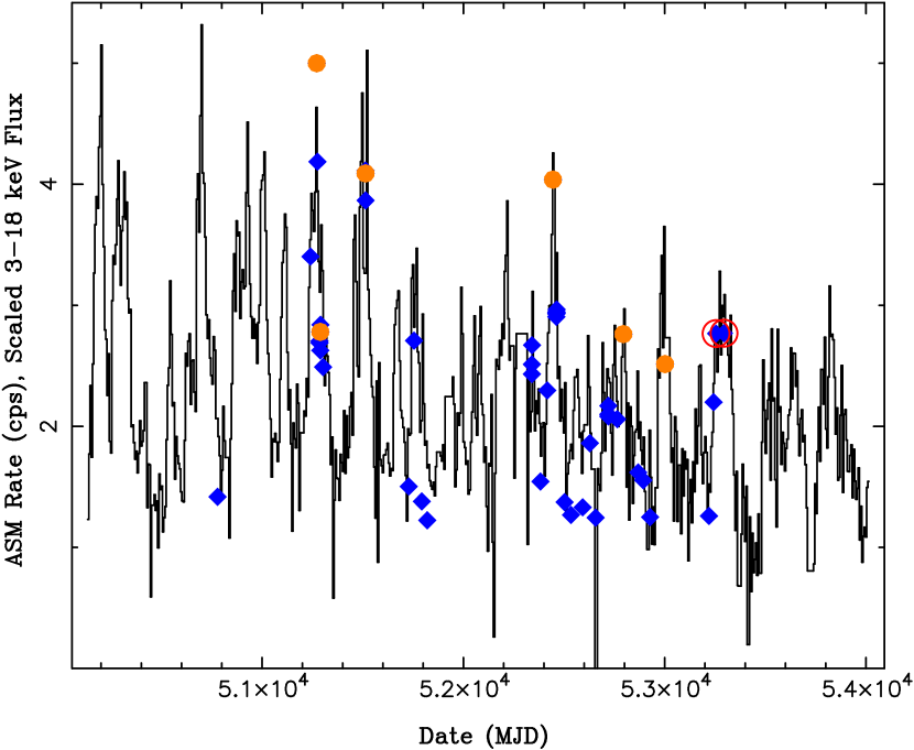
Figure 8.— All Sky Monitor lightcurve for 4U 1957+11  with scaled 3-18 keV PCA flux from pointed observations overlaid. RXTE observations simultaneous with Chandra and XMM-Newton are circled. Circles here and in subsequent figures represent observations where 4U 1957+11 was transiting to ‘steep power-law state’ behavior.

As discussed by Nowak & Wilms (1999) and Wijnands, Miller & van der Klis (2002), the RXTE data of 4U 1957+11 can be well-described by a model that consists of a combination of a multi-temperature disk spectrum, a power-law, and a gaussian line. For most of the RXTE observations the line peaks at an amplitude of $\mathrel{\hbox to0.0pt{\raise 2.20013pt\hbox{$<$}\hss}{\lower 2.20013pt\hbox{$\sim$}}}2$–$3\%$ of the local continuum level, and it is statistically required by the data. No such line was present in either the Chandra or the XMM-Newton observation (line flux $\mathrel{\hbox to0.0pt{\raise 2.20013pt\hbox{$<$}\hss}{\lower 2.20013pt\hbox{$\sim$}}}7\times 10^{-5}$ ph cm^-2 s^-1). There are several possibilities for this discrepancy, and perhaps some combination of all are at play. With its $\approx 1\,{\rm deg}^{2}$ effective field of view, the PCA will detect diffuse galactic emission which shows a prominent 6.7 keV line. Based upon scalings between the PCA line flux and the DIRBE 4.9 $\mu$m infrared flux (Revnivtsev, Molkov & Sazonov, 2006), one expects an RXTE-detected line amplitude of $\approx 4\times 10^{-5}$ ph cm^-2 s^-1 (i.e., approximately 10% of the observed line) at the Galactic coordinates of 4U 1957+11 ($l=51.307^{\circ}$, $b=-9.330^{\circ}$). Remaining systematic uncertainties in the PCA response matrix may be as large as 1% of the continuum level in the Fe line region, which could account for a line amplitude of $\mathrel{\hbox to0.0pt{\raise 2.20013pt\hbox{$<$}\hss}{\lower 2.20013pt\hbox{$\sim$}}}1.5\times 10^{-4}$ ph cm^-2 s^-1 for the observations simultaneous with Chandra and XMM-Newton. The remaining 50% of the line flux for these latter two observations, which is still three times larger than the Chandra and XMM-Newton upper limits, may be real and could be indicative of the greater sensitivity of PCA to weak and broad line features. Such a broad line would have been detectable by Chandra and XMM-Newton only if their own systematic uncertainties were at the 1% level, and we have already noted larger broad band discrepancies between the HEG and MEG.

Table 4kerrbb+comptt+gaussian Fits to Selected RXTE Data

ID	$a$	${\rm\dot{M}}$	${\rm h_{d}}$	${\rm D_{BH}}$	${\rm A_{comptt}}$	$\tau_{\rm p}$	${\rm A_{line}}$	$\sigma_{\rm line}$	$\chi^{2}/$dof
		($10^{17}~{}{\rm g~{}s^{-1}}$)		(kpc)	$(10^{-5})$		$(10^{-4})$	(keV)
40044-01-02-01	$0.99026^{+0.00473}_{-0.00000}$	$0.749^{+0.171}_{-0.113}$	$0.929^{+0.045}_{-0.043}$	10	$263.7^{+7.5}_{-8.5}$	$0.19^{+0.02}_{-0.01}$	$5.4^{+4.6}_{-3.0}$	$0.5^{+0.5}_{-0.5}$	18.0/27
	$0.99409^{+0.00581}_{-0.99409}$	$1.541^{+4.817}_{-0.761}$	1.7	$15.1^{+56.1}_{-2.8}$	$264.0^{+7.5}_{-10.4}$	$0.19^{+0.02}_{-0.01}$	$5.5^{+5.2}_{-3.1}$	$0.5^{+0.5}_{-0.5}$	18.0/27
	$0.59987^{+0.08325}_{-0.08022}$	$3.556^{+0.471}_{-0.452}$	1.7	10	$254.2^{+7.9}_{-16.5}$	$0.20^{+0.01}_{-0.02}$	$4.3^{+3.9}_{-2.2}$	$0.3^{+0.4}_{-0.3}$	19.0/28
70054-01-11-00	$0.99896^{+0.00002}_{-0.00009}$	$0.349^{+0.001}_{-0.001}$	$1.102^{+0.002}_{-0.003}$	10	$0.0^{+0.2}_{-0.0}$	$0.01^{+4.99}_{-0.00}$	$3.9^{+0.4}_{-0.6}$	$0.8^{+0.2}_{-0.2}$	16.7/17
	$0.99986^{+0.00001}_{-0.00001}$	$1.161^{+0.002}_{-0.004}$	1.7	$19.5^{+0.1}_{-0.0}$	$4.6^{+0.2}_{-0.4}$	$0.01^{+0.01}_{-0.00}$	$7.1^{+0.4}_{-0.7}$	$1.0^{+0.0}_{-0.1}$	25.7/17
	$0.82851^{+0.00334}_{-0.01372}$	$1.414^{+0.035}_{-0.019}$	1.7	10	$0.0^{+0.4}_{-0.0}$	$0.01^{+4.99}_{-0.00}$	$4.5^{+1.7}_{-1.0}$	$0.7^{+0.2}_{-0.2}$	46.5/18
90123-01-03	$0.99969^{+0.00021}_{-0.01854}$	$0.576^{+0.467}_{-0.017}$	$1.087^{+0.017}_{-0.014}$	10	$5.6^{+4.6}_{-5.1}$	$0.02^{+2.50}_{-0.01}$	$4.7^{+1.9}_{-1.5}$	$0.5^{+0.3}_{-0.4}$	25.0/25
	$0.99974^{+0.00012}_{-0.00014}$	$2.676^{+0.154}_{-0.016}$	1.7	$21.7^{+0.4}_{-0.1}$	$6.0^{+0.7}_{-3.0}$	$0.01^{+4.99}_{-0.00}$	$4.6^{+0.8}_{-0.8}$	$0.5^{+0.2}_{-0.2}$	24.9/25
	$0.84529^{+0.00236}_{-0.00463}$	$2.412^{+0.033}_{-0.029}$	1.7	10	$0.0^{+2.1}_{-0.0}$	$0.37^{+4.63}_{-0.36}$	$9.0^{+1.5}_{-1.5}$	$0.7^{+0.1}_{-0.1}$	48.0/26
90063-01-01	$0.99852^{+0.00019}_{-0.00312}$	$0.655^{+0.042}_{-0.021}$	$1.113^{+0.021}_{-0.011}$	10	$6.2^{+0.8}_{-0.1}$	$0.01^{+0.68}_{-0.00}$	$5.1^{+1.6}_{-1.7}$	$0.6^{+0.2}_{-0.3}$	18.8/25
	$0.99795^{+0.00050}_{-0.00268}$	$3.708^{+0.474}_{-0.472}$	1.7	$23.3^{+0.2}_{-1.5}$	$5.2^{+1.7}_{-3.8}$	$0.03^{+4.97}_{-0.02}$	$5.1^{+1.8}_{-1.7}$	$0.6^{+0.2}_{-0.3}$	18.8/25
	$0.84516^{+0.00203}_{-0.00401}$	$2.415^{+0.035}_{-0.026}$	1.7	10	$0.0^{+2.3}_{-0.0}$	$2.50^{+2.50}_{-2.49}$	$8.7^{+1.6}_{-1.3}$	$0.7^{+0.1}_{-0.1}$	39.0/26

Note. — One fit used a fixed mass of 3 M_⊙, a fixed distance of 10 kpc, and a variable spectral hardening factor, another set used a fixed mass of 16 M_⊙, a fixed spectral hardening factor of 1.7, and a variable distance, and the third set a fixed mass of 3 M_⊙, a fixed distance of 10 kpc, and a fixed spectral hardening factor of 1.7. Line normalization, ${\rm A_{line}}$, is total photons/cm²/s in the line. 0.5% systematic errors were added in quadrature to the data. Error bars are 90% confidence level.

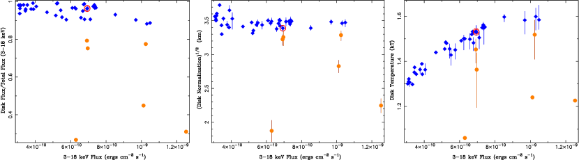
Figure 9.— Left: The fraction of disk flux to total flux, in the 3-18 keV energy band, for diskbb+powerlaw fits to 4U 1957+11. Middle: Square root of disk normalization vs. PCA flux for diskbb+powerlaw fits to RXTE observations of 4U 1957+11. Right: Disk temperature vs. PCA for diskbb+comptt fits to 4U 1957+11.

For the disk plus power-law fits, we constrained the power-law photon index, $\Gamma$, to lie between 1–3, but let the power-law normalization freely vary. These fits were fairly successful overall (reduced $\chi^{2}$ ranged from 0.5–2, and averaged 1). Parameter trends with observed flux are shown in Fig. 9, and show several features of interest. First, the vast majority of the observations are consistent with having a nearly constant disk normalization, which one could take as a proxy for disk radius. At the low end of 3–18 keV flux, the disk normalization/radius turns upward. Phenomenologically, such observed increases in disk radius have been associated with low luminosity transitions to the hard state (e.g., see the similar behavior of LMC X-3; Wilms et al., 2001), which we expect to occur near 3% of the Eddington luminosity (Maccarone, 2003). It is therefore possible that our lowest luminosity observations are near such a transition at 3% ${\rm L_{Edd}}$. (On the other hand, Saito et al. 2006 note a similar increase in fitted disk radius for GRO J1655$-$40, without any associated transition, or near transition, to a low/hard state.)

Second, we see that as the 3–18 keV flux increases, the fraction of the flux contributed by the power-law slightly increases. Half a dozen points, however, show a much more significant contribution by the power-law (Fig. 9). At the same time, those observations show a dramatic decrease in the disk normalization. Each of those observations is associated with peaks in the ASM lightcurve, and several are associated with high variability, including one instance of “rapid state transitions” (see §4.2). We identify those observations with what Remillard & McClintock (2006) refer to as the “steep power-law” state (or, the “very high state”; Miyamoto et al. 1993).

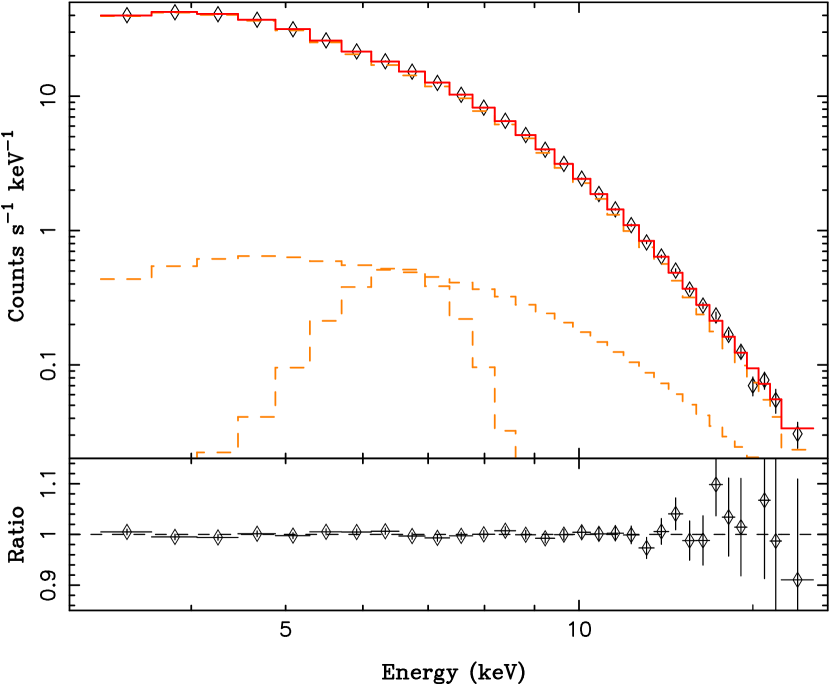
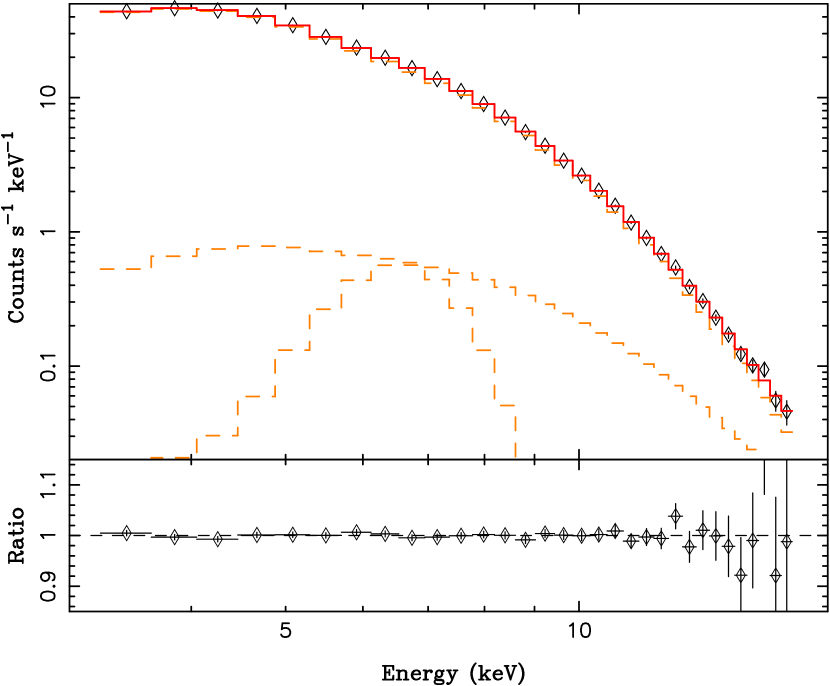
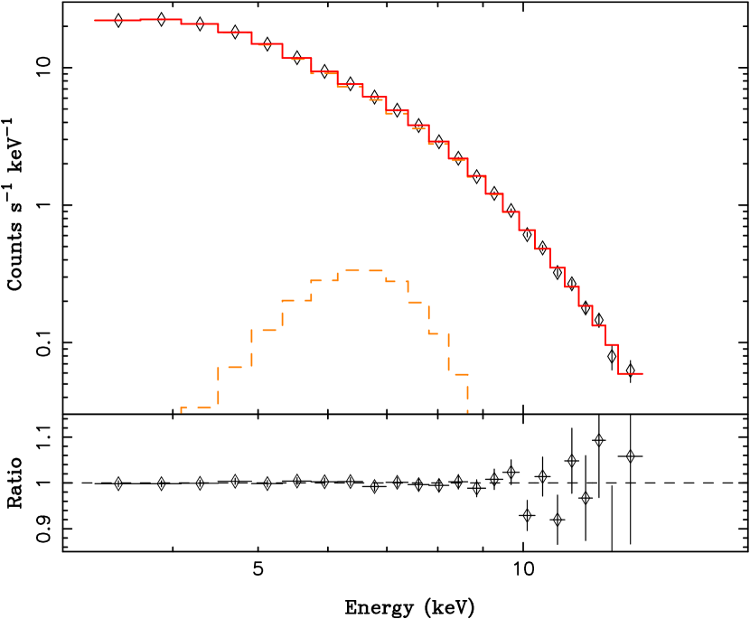
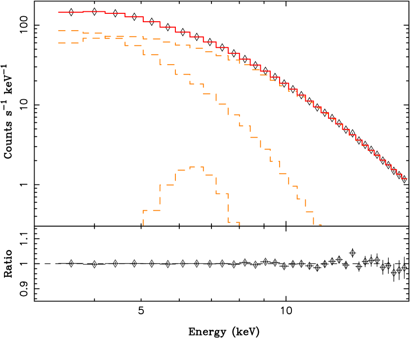
Figure 10.— Count rate spectra for the RXTE observations simultaneous with Chandra (top left) and XMM-Newton (top right), and for the softest/faintest (bottom left) and hardest/brightest (bottom right) of the RXTE observations, all fit with the kerrbb+comptt+gaussian model (3 ${\rm M_{\odot}}$, 10 kpc, and freely varying color correction fraction). Dashed lines show the individual model components folded through the detector response.

Even though the disk normalization drops and the power-law flux increases for the disk plus power-law fits, the fitted disk temperature does not show any significant deviations from a trend of 3–18 keV flux $\propto(kT)^{5}$ (not shown in Fig. 9). For a disk spectrum with constant disk radius, we expect the bolometric flux to scale $\propto(kT)^{4}$, and, for these temperatures, to scale approximately as $(kT)^{5}$ in the 3–18 keV bandpass. This same relation between disk temperature and 3–18 keV flux holds if we instead fit the spectra with a disk plus Comptonization spectrum, as shown in Fig. 9.

For these latter fits, we model the spectrum in the same manner as in §3: we use a diskbb + comptt model and tie the seed photon temperature to the disk peak temperature, freeze the corona temperature to 50 keV, but let the coronal spectrum normalization and optical depth (constrained by $0.01<\tau_{\rm p}<5$) be fit parameters. Results for several of these fits are presented in Table 3. The majority of the observations again show a nearly constant disk radius, and a 3–18 keV flux that scales approximately $\propto(kT)^{5}$. The Comptonization models, however, now show the half dozen ‘steep power-law state’ observations as being associated with dramatic drops in the disk/seed photon temperatures (Fig. 9).

We now consider fits where the unphysical diskbb component is replaced with the kerrbb model. As for the fits to the Chandra data, we fix the disk inclination to 75^∘, and set the source distance to 10 kpc and the black hole mass to 3 ${\rm M_{\odot}}$. The latter choices are motivated by our faintest RXTE observation for which we measure a 3–18 keV absorbed flux of $3.1\times 10^{-10}~{}{\rm ergs~{}sec^{-1}~{}cm^{-2}}$. Taking the diskbb model at face value, with an inclination of $75^{\circ}$, this result translates to an unabsorbed bolometric luminosity of 3% ${\rm L_{Edd}}$ for this presumed mass and distance. The black hole is unlikely to be less massive than 3 ${\rm M_{\odot}}$, and low black hole masses lead to higher disk temperatures. Thus, we see these parameter choices as minimizing the need for high spin parameters in the kerrbb fits, with 10 kpc then being a lower limit to the source distance.

The remaining kerrbb fit parameters are the accretion rate, $\dot{\rm M}$, the black hole spin, $a^{*}$, and the disk atmosphere color-correction factor, ${\rm h_{d}}$. The kerrbb model does not fit a disk temperature per se; therefore, we set the input seed photon temperature of the comptt model equal to the diskbb peak temperature from our previous fits (see Davis, Done & Blaes, 2006). As before, we also freeze the coronal temperature to 50 keV, and constrain the optical depth to lie between 0.01–5. Selected fit results are presented in Table 4 and Fig. 10.

Even with choosing a very low black hole mass, and thus naturally favoring higher disk temperatures, the kerrbb models uniformly prefer to fit $a^{*}\approx 1$. On the other hand, the disk atmosphere spectral hardening remains low, with ${\rm h_{d}}\approx 1.1$. There is a slight trend for ${\rm h_{d}}$ to decrease with increasing flux, as shown in Fig. 11. For some of the observations where the disk contribution to the total flux dramatically decreased, ${\rm h_{d}}$ drops slightly lower still. This is not surprising as the inclusion of a coronal component can qualitatively replace the need for hardening from the disk atmosphere.

The kerrbb model has a number of parameter degeneracies which we can exploit to search for fits with the more usual color-correction factor of ${\rm h_{d}}=1.7$. Specifically, the apparent temperature increases $\propto{\rm h_{d}}$, and $\propto(\dot{\rm M}/{\rm M}^{2})^{1/4}$. If we increase ${\rm h_{d}}$, then in order to retain roughly the same spectral shape we must decrease $({\rm\dot{M}}/{\rm M}^{2})^{1/4}$. Solely decreasing ${\rm\dot{M}}$, however, makes our faintest observation less than 3% ${\rm L_{Edd}}$. Additionally, the source distance would need to be reduced $\propto{\rm\dot{M}}^{1/2}$ in order to retain the same observed flux. We would have expected to detect a transition to a hard spectral state if ${\rm\dot{M}}$ were lower than we have assumed. In order to keep our faintest observation at $\approx 3\%$ ${\rm L_{Edd}}$, we must instead scale ${\rm M}\propto{\rm h_{d}}^{4}$, $\dot{\rm M}\propto{\rm h_{d}}^{4}$, and the source distance as $\propto{\rm h_{d}}^{2}$. A consistent picture may be obtained with ${\rm h_{d}}=1.7$, if $M\approx 16$ ${\rm M_{\odot}}$ and the distance to the source is $\approx 22$ kpc.

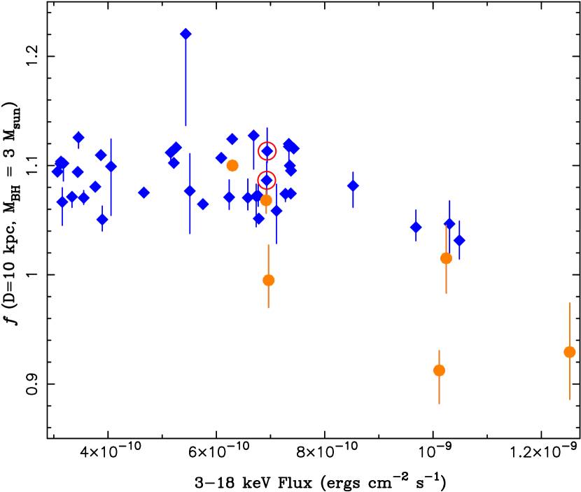
Figure 11.— Spectral hardening factor vs. PCA flux for kerrbb+comptt fits to 4U 1957+11. We assume a black hole mass of 3 ${\rm M}_{\odot}$, a distance of 10 kpc, and an inclination of 75^∘.

We searched for a set of kerrbb+comptt fits where we froze the disk color-correction factor at ${\rm h_{d}}=1.7$, the black hole mass at 16 ${\rm M_{\odot}}$, but let the disk accretion rate, $\dot{\rm M}$, spin parameter, $a^{*}$, and source distance all be free parameters. Clearly, the source distance cannot truly be physically changing in a perceptible way; however, the degree to which we obtain a uniform set of fitted distances might provide a self-consistency check on the use of the kerrbb model. Selected results from these fits are presented in Table 4, and the fitted distances vs. 3–18 keV flux are presented in Fig. 12. In general, these fits work every bit as well as the 3 ${\rm M_{\odot}}$, 10 kpc fits. The lower flux observations cluster about a fitted distance of $\approx 22$ kpc. There is a trend, however, for the fitted distances to decrease with higher fluxes, and for several of the ‘steep power-law state’ observations to fit distances as low as 15 kpc.

We have considered another class of fit degeneracy: disk atmosphere hardening factor and spin. Here we again freeze the black hole mass to 3 ${\rm M_{\odot}}$ and the distance to 10 kpc, but freeze the hardening factor to ${\rm h_{d}}=1.7$. As more of the peak in the apparent temperature is being attributed to the color-correction factor, the disk spin must be decreased, thereby decreasing the accretion efficiency and increasing the radius of the emitting area near the peak temperatures. To maintain the same observed flux, the accretion rate must be increased above that for the models with lower ${\rm h_{d}}$. Formally, these are significantly worse fits than our previous ones, with a mean $\Delta\chi^{2}=22$. I.e., an increased accretion rate and spectral hardening factor are not acting as simple proxies for high spin in these models. (In terms of fractional residuals, however, the fits are somewhat reasonable.)

As shown in Fig. 13, these fits yield a relatively uniform spin of $a^{*}\approx 0.84$, with a slight trend for fitted spin to increase with increasing flux. Notable exceptions to this behavior are seen, however, as some of the ‘steep power-law state’ observations fit much reduced black hole spins. Again, this is a contribution from a Comptonization component, which is strong for these observations, replacing some of the need for spectral hardening due to rapid spin.

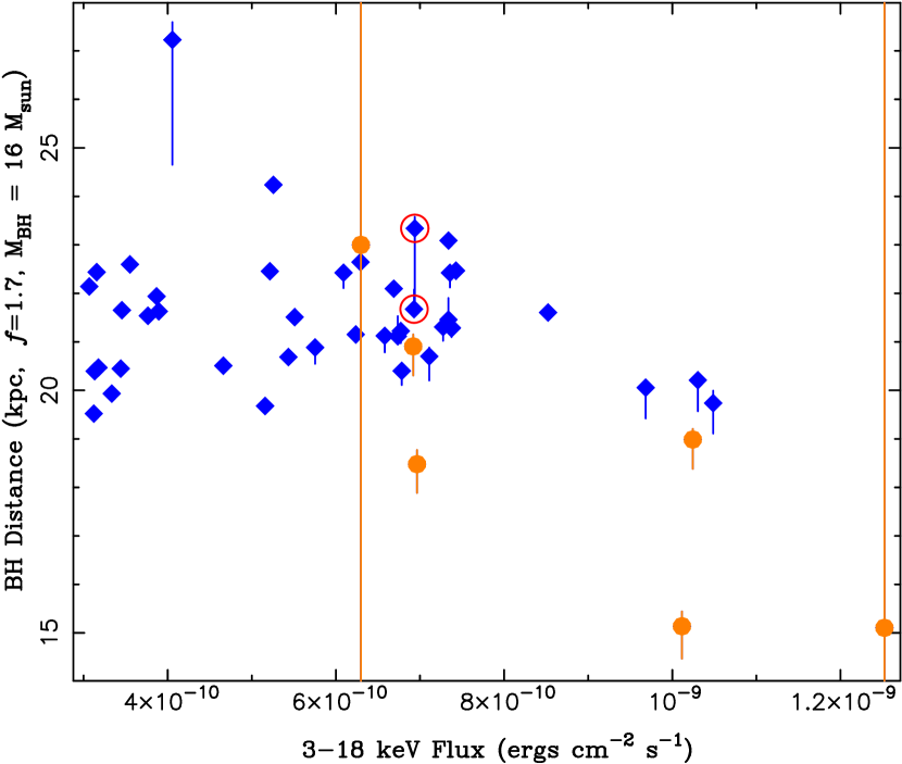
Figure 12.— Fitted black hole distance for kerrbb+comptt fits to 4U 1957+11, assuming a spectral hardening factor of ${\rm h_{d}}=1.7$, a black hole mass of 16 ${\rm M}_{\odot}$, and an inclination of 75^∘.

Note that we did search for a set of disk atmosphere model fits where we kept the source mass low ($3\,{\rm M}_{\odot}$) and moved the distance further out (17 kpc) while fitting higher accretion rates, to intrinsically increase the disk temperatures and raise the implied fractional Eddington luminosities by a factor of $\approx 3$. These models failed completely, with best fit $\chi^{2}$ values increasing by factors of almost 3 over high-spin models. We again find that high-spin is not simply degenerate with increased accretion rate in the models. Essentially this is because high-spin adds an inner disk region with high temperature and high flux (approximately tripling the flux when going from non-spinning to Kerr solutions), which leads to a strong, broad component in the high energy spectrum. High accretion, low spin models, fail to reproduce such broad, high energy PCA spectra.

4.2. Variability

The study of the rapid variability properties of 4U 1957+11 was performed using high time resolution data from the PCA. We created power spectra from the entire PCA energy band ($\approx$2–60 keV), covering the 2^-7–2048 Hz frequency range. Observations with high disk fractions ($>$80%, as defined by Fig. 9) typically showed weak or no significant variability. Combining these observations resulted in a power spectrum that could be fitted reasonably well by a single power-law component ($\chi^{2}$/dof=101.0/79). This fit improved significantly ($\chi^{2}$/dof=73.1/74) by adding two Lorentzians, one (with Q-value fixed at 0 Hz) for a weak band-limited noise component around 2 Hz and the other for a QPO at 25 Hz. The resulting parameters from the fit are listed in Table 5. Note, that although the improvement in the fit is statistically significant, the two added components are only marginally significant themselves ($\approx 3\sigma$).

Observations with lower disk fractions showed an increase in variability, with maximum of 12.1$\pm$0.6% root mean square (rms) variability (0.01–100 Hz) in the observation with the lowest disk fraction (ObsID 50128-01-09-00; disk fraction of $\approx$30%; see Fig. 14). Combining the power spectra of all observations with disk fractions lower than 80% and fitting with the same model as above, we find that all variability components increased in strength (see Table 5).

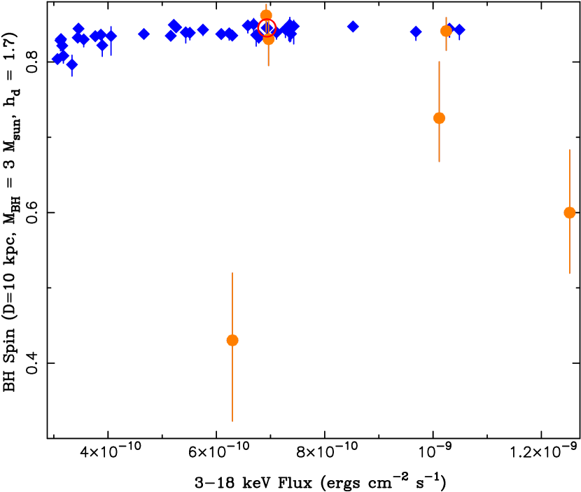
Figure 13.— Fitted black hole spin for kerrbb+comptt fits to 4U 1957+11, assuming a spectral hardening factor of ${\rm h_{d}}=1.7$, a black hole mass of 3 ${\rm M}_{\odot}$, a distance of 10 kpc, and an inclination of 75^∘.

The power spectral properties of the high- and low-disk fraction observations are consistent with the soft state and the soft end of the transition between the hard and soft states, respectively. Observation of such variability strengthens the argument that 4U 1957+11 is indeed a black hole, and not a neutron star. The frequencies of the QPOs are similar to that seen in a few other black hole systems when they were in or close to their soft state, e.g. XTE J1550$-$564 (Homan et al., 2001) and GRO J1655$-$40 (Sobczak et al., 2000). The comparable frequencies observed in these latter two sources have ranged from 15–22 Hz, and futhermore the spectra of these sources have been fit with disk models that imply black hole spins in the range of $a^{*}\approx 0.1$–0.8 (Davis, Done & Blaes, 2006; Shafee et al., 2006). Thus, if such variability features are related to black hole spin, a consistent picture arises between their spectral and variability results.

In two of the low-disk fraction observations (ObsIDs 40044-01-02-01 and 70054-01-04-00) we observed fast changes in the count rate, which resemble the dips/flip-flops observed in other black hole X-ray binaries during transition from the hard to the soft state (e.g., Miyamoto et al., 1991). In 4U 1957+11, these changes in the count rate were accompanied by moderate changes in the spectral variability properties, but count rates were too low to classify the power spectra in the high and low count rate phases independently.

5. Discussion

We have presented observations of the black hole candidate 4U 1957+11 performed with the Chandra, XMM-Newton, and RXTE X-ray observatories. All of these observations point toward a relatively simple and soft spectrum, indicative of a classic BHC disk-dominated soft state. The Chandra and XMM-Newton spectra, especially at high resolution, indicate a remarkably unadulterated disk spectrum. That is, the absorption of the spectrum is very low at only ${\rm N_{H}}=1$–$2\times 10^{21}\,{\rm cm}^{-2}$, and with the possible exception of an unidentified line at 21.8 Å, there is very little evidence of spectral complexity intrinsic to the source. From that vantage point, 4U 1957+11 may be the cleanest disk spectrum with which to study modern disk atmosphere models.

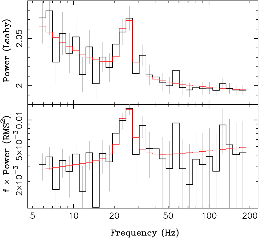
Figure 14.— An approximately 25 Hz quasi-periodic oscillation seen in the 4.5-27.5 keV 4U 1957+11 lightcurve from ObsID 50128-01-09-00, the observation with the smallest disk contribution to the observed 3-18 keV flux. The top panel shows the power spectrum with the Poisson noise level unsubtracted and normalized to $\approx 2$. The bottom panel shows Fourier frequency times the power spectrum, now with the Poisson noise level subtracted and the PSD normalized to (root mean square)²/Hz.

Table 5Power spectra fit parameters

Parameter	High Disk Frac.	Low Disk Frac.
PL rms (%)	1.05$\pm$0.09	2.6${}^{+0.7}_{-0.5}$
PL index	1.57$\pm$0.15	0.92$\pm$0.12
BLN rms (%)	1.2$\pm$0.2	4.1${}^{+1.1}_{-0.7}$
BLN $\nu_{max}$ (Hz)	1.9${}^{+1.5}_{-0.8}$	13${}^{+9}_{-5}$
QPO rms (%)	2.0$\pm$0.3	3.4$\pm$0.9
QPO Q-value	2.10${}^{+1.24}_{-0.76}$	2.5${}^{+3.6}_{-1.1}$
QPO $\nu_{max}$ (Hz)	25.0$\pm$2.2	29.5$\pm$2.1
total rms	2.7$\pm$0.4	6.1$\pm$0.4
$\chi^{2}$/dof	73.1/74	65.9/80

Perhaps the one indication of additional, unmodeled spectral complexity is the fact that the broadband fits and the more localized, high resolution edge and line fits yield (low) neutral columns that differ from each other by a factor of two. This, along with the 21.8 Å  absorption feature might indicate the presence of other weak, unmodeled spectral components at very soft X-ray energies. Even if this were the case, this is to be compared to other BHC to which such atmosphere models have been applied, e.g., GRO J1655$-$40 (Shafee et al., 2006), where there is both a larger neutral column (${\rm N_{H}}=7\times 10^{21}\,{\rm cm^{-2}}$), a complex Fe K$\alpha$ region (modeled with both emission and smeared edges by Shafee et al. 2006) and high resolution observations of intermittently present, complex X-ray spectral features that are local to the system (i.e., Miller et al., 2006, 2008). In comparison, the 4U 1957+11 spectrum, even with its uncertainties, is much simpler.

The observations presented here strengthen the case that 4U 1957+11 is a black hole system. The spectrum closely matches a classic, soft state disk spectrum (well-modeled by diskbb), with a contribution from a harder, non-disk component that generally increases as the flux increases. Occasionally (a half dozen observations), the contribution from this hard component increases, the X-ray variability increases, a possible QPO is observed, and we even observe lightcurve ‘dipping’ and ‘flip-flop’ behavior (Miyamoto et al., 1991, 1993). All of this is behavior familiar from studies of other BHC (Homan et al., 2001, and references therein). Unfortunately, observation of these behaviors provides little strong input to estimates of the system parameters, i.e., mass, distance, and inclination. ‘Flip-flop’ behavior has often been associated with luminosities of a few tens of percent (Miyamoto et al., 1991, 1993; Homan et al., 2001), which is higher than we have presumed for the fits described here. The threshold luminosity for such behavior, however, is not firm, and we further note that high accretion rate/large distance fits to the PCA spectra failed (§4.1). The fact that we do not see a transition to a BHC hard state— although we may see some indications from increases in the fitted disk radius at low luminosity— strongly suggest that the mass is $>3\,{\rm M_{\odot}}$ and the distance is $>10$ kpc.

Despite the fact that we do not have a firm estimate of mass and distance for 4U 1957+11, the relativistic disk models still strongly statistically prefer rapid spin solutions. Essentially, this is because the diskbb models fit very high temperatures – as high as 1.7 keV – with fairly low normalizations. We saw, however, that for the Chandra observation, or for the RXTE observations where the power-law/Comptonization component strengthens, the need for spectral hardening of the disk, either via a color-correction factor (${\rm h_{d}}$) or rapid spin, was greatly reduced. Phenomenologically, a coronal component can mimic the effects of rapid spin. This naturally leads to the question of whether or not one is sure that any residual coronal component completely vanishes at low flux. Does one ever observe a “bare” disk spectrum?

It is a rather remarkable fact that the Chandra observation, and the low flux RXTE observations, are mostly described via three parameters: absorption, diskbb temperature, and diskbb normalization. Even more remarkably, changes in the spectrum, both in terms of amplitude and overall shape, are mainly driven by variations of only one parameter: diskbb temperature. The relativistic disk models, on the other hand, must ascribe essentially this one parameter to a combination of four parameters: $a^{*}$, disk inclination (which affects the appearance of relativistic features), $({\rm\dot{M}/M}^{2})$, and ${\rm h_{d}}$. In principle, any of the latter three can vary among observations. (Disk inclination can vary due to warping; see Pringle 1996.) Unfortunately, there is no truly unique, sharp feature in the high resolution spectrum that completely breaks degeneracies among these parameters. The overall magnitude of the diskbb temperature and shape of the 4U 1957+11 spectra, however, seem best reproduced with the most rapid spin models; simply increasing accretion rates or spectral hardening factors is insufficient to model the spectra fully.

We do not see the essential question as being whether or not 4U 1957+11 is rapidly spinning. Instead, we view the more observationally motivated and perhaps more fundamental question as being: why is the characteristic disk temperature of 4U 1957+11 so high? Rapid spin is one hypothesis. Another would be that there is indeed a residual, low temperature corona, even at low flux. The possibly high inclination of this source ($\approx 75^{\circ}$ to be consistent with optical lightcurve variations, while being consistent with the lack of X-ray eclipses) would mean that we are viewing the disk through a larger scattering depth than would be usual for most BHC in the soft state. We also note that there exists very little, self-consistent theoretical modeling of low temperature Comptonizing coronae with high temperature (1–2 keV) seed photon temperatures. Most energetically balanced, self-consistent models (e.g., Dove, Wilms & Begelman, 1997) have focused on high coronal temperatures (50–200 keV) with low seed photon temperatures (100–300 eV).

If one is to take the rapid spin hypothesis for the high diskbb temperature at face value, then these observations offer something of a prediction. Statistically, they do prefer rapid spin, and based upon observations of other BHC we would have expected to observe a hard state if the faintest observations were $\mathrel{\hbox to0.0pt{\raise 2.20013pt\hbox{$<$}\hss}{\lower 2.20013pt\hbox{$\sim$}}}3\%\,{\rm L_{Edd}}$. If the theoretically preferred value of the spectral hardening factor is indeed ${\rm h_{d}}=1.7$, future measurements should find 4U 1957+11 to be an $\approx 16\,{\rm M_{\odot}}$ black hole at $\approx 22$ kpc. Whether or not this turns out to be the case, given the nature of 4U 1957+11 as perhaps the simplest, cleanest example of a BHC soft state, observations to independently determine this system’s parameters (mass and distance) are urgently needed.

In this appendix, we describe how we model the mild pile up that is present in the MEG and, to lesser degree, the HEG data. Our model follows the discussions of Davis (2001) and Davis (2003), although we do not attempt to arrive at an ab initio description of pile up. Instead, we present a simple, phenomenological description where the absolute amplitude of pile up is left as a fit parameter (albeit one that can be determined roughly with empirical knowledge and then frozen at a fixed value, or fitted with a limited range of “acceptable” values). In contrast to spectral pile up solely with the CCD detector, where piled events can reappear in the spectrum at higher implied energies, gratings pile up (at least in $1^{\rm st}$ order spectra) can be thought of as a straight loss of events. Whether the piled events ‘migrate’ to bad grades, or are read as a single event of higher energy and are thus removed from the ‘order sorting window’, it is still a simple loss term (Davis, 2003).

The degree of loss due to pile up scales with $C_{i}$, the number of expected incident events in a given detector region per detector frame integration time. The detected number of events is then reduced by a factor $\exp({\cal A}C_{i})$, for a suitably chosen region and where ${\cal A}$ is a ‘fudge factor’ of order unity. The proper detector region to consider is approximately 3 pixels in the ‘cross dispersion’ direction, by a 3–5 pixel length along the dispersion direction of the gratings arm being analyzed. (Events in a single frame that land in adjacent pixels will always be piled, while events that are removed from one another by four pixels will only be piled if their charge clouds extend toward one another; see Davis 2003.) Given that the peak effective area of the MEG is approximately twice that of the HEG, and the fact that detector pixels cover twice the wavelength range in the MEG, we expect the pile up to be approximately 4 times larger in the MEG.

It is important to note that one needs to consider all events in a given detector region, i.e., all spectral orders, background events, contributions from the wings of the $0^{\rm th}$ order point spread function, etc., whether or not these events are otherwise rejected by order sorting. To partly account for this necessity, the pile up model described here uses information from the $2^{\rm nd}$ and $3^{\rm rd}$ order ancillary response functions (arfs). Specifically, we create a ‘convolution model’ where, given an input spectrum, we define $C_{i}(\lambda)$ as the first order arf multiplied by the unpiled model spectrum (yielding counts per detector bin). We further increase $C_{i}(\lambda)$ by multiplying the unpiled model by the $2^{\rm nd}$ order arf, then shifting the $2^{\rm nd}$ order wavelengths by a factor of two, and then rebinning and adding this contribution to $C_{i}(\lambda)$. A similar procedure is used for the $3^{\rm rd}$ order contribution. We then use the input pile up fraction fit parameter, $p_{f}$, to normalize the exponential reduction of the spectrum. Specifically, we multiply the counts per bin predicted for the unpiled model by $\exp[\log(1-p_{f})[C_{i}(\lambda)/\max(C_{i})]]$.

There are two important subtleties to address. First, in certain regions of the spectrum, specifically those wavelength regions that are dithered over chip gaps or detector bad pixels, the counts are lower not due to a low intrinsic flux, but rather due to a fractionally reduced exposure. The FRACEXPO column found in the arf FITS files for Chandra gratings data provides this information; therefore, we can approximately correct for this effect. Second, for Chandra gratings spectra, a portion of the detector area information is contained within the response matrix files (rmf), which are not normalized to unity. In practice, before fitting the pile up model, we renormalize the gratings $1^{\rm st}$ order arfs using the ISIS functions factor_rsp, get_arf, and put_arf. Assuming a_id is the data index of the $1^{\rm st}$ order arf, and r_id is the data index of the $1^{\rm st}$ order rmf, we proceed as follows in ISIS:

   isis> a = get_arf(a_id);        % Read the existing arf into a structure
   isis> na_id = factor_rsp(r_id); % Factor the rmf into normalized rmf*arf
   isis> na = get_arf(na_id);      % Read the new, factored arf component
   isis> a.value *= na.value;      % Multiply original arf by factored value
   isis> put_arf(a_id, na);        % Replace old arf value with rescaled value
   isis> delete_arf(na_id);        % Delete the factored arf component

It is precisely because ISIS has the ability to read and manipulate information from all input data files, and then easily mathematically manipulate this information to create new functionality, that we are able to define a relatively simple pile up correction model.

Ideally, we should incorporate additional information, such as the variation of the line spread function (LSF; i.e., the cross dispersion profile) along the gratings arms, the 5–10% of the events that are typically excluded by order sorting, etc. For these reasons we cannot assign an absolute estimate of the pile up fraction. However, to the extent that we have correctly captured the relative changes of total count rate along the dispersion direction, and have chosen a suitable peak pile up fraction, we should have a reasonably accurate pile up correction as a function of wavelength. More sophisticated ab initio models currently are under development (J. Davis, priv. comm.).

For our data, the peak of the detected MEG count rate (including contributions from $2^{\rm nd}$ and $3^{\rm rd}$ order events) occurs in the 6–8 Å region, and peaks at a value of $\approx$ 0.08 counts/frame/3 pixels. Thus, making a simple first order correction since this rate already includes pile up, and including up to 5 pixels, we expect a peak pile up fraction in the 0.09–0.16 range. We could have chosen a value in this range and have frozen it in the fits, but the fitted values fall within the middle of these estimates. Likewise, for the HEG spectra we estimate a peak pile up fraction of 0.025–0.036. Such fractions are comparable to or smaller than existing systematic uncertainties in the Chandra calibration. Additionally, we found a great deal of degeneracy in any attempts to fit the HEG value directly, thus we froze peak the pile up fraction at a value of 0.03.

The S-lang code that we used to define a simple gratings pile up model as an ISIS user model is presented in the electronic version of this manuscript.

define simple_gpile_fit(lo,hi,par,fun)
{
   % Peak pileup correction goes as:
   %    exp(log(1-pfrac)*[counts/max(counts)])

   variable pfrac = par[0];

   % Pileup scales with model counts from *data set* indx ...
   variable indx = typecast(par[1],Integer_Type);

   if( indx == 0 or pfrac == 0. )
   {
      return fun;   % Quick escape for no changes ...
   }

   % ... but the arf index could be a different number, so get that

   variable arf_indx = get_data_info(indx).arfs;

   % Get arf information

   variable arf = get_arf(arf_indx[0]);

   % In dither regions (or bad pixel areas), counts are down not
   % from lack of area, but lack of exposure.  Pileup fraction
   % therefore should scale with count rate assuming full exposure.
   % Use the arf "fracexpo" column to correct for this effect

   variable fracexpo = get_arf_info(arf_indx[0]).fracexpo;
   if( length(fracexpo) > 1 )
   {
      fracexpo[where(fracexpo ==0)] = 1.;
   }
   else if( fracexpo==0 )
   {
      fracexpo = 1;
   }

   % Rebin arf to input grid, correct for fractional exposure, and
   % multiply by "fun" to get ("corrected") model counts per bin

   variable mod_cts;
   mod_cts = fun * rebin( lo, hi,
                          arf.bin_lo, arf.bin_hi,
                          arf.value/fracexpo*(arf.bin_hi-arf.bin_lo) )
                / (hi-lo);

   % Go from cts/bin/s -> cts/angstrom/s

   mod_cts = mod_cts/(hi-lo);

   % Use 2nd and 3rd order arfs to include their contribution.
   % Will probably work best if one chooses a user grid that extends
   % from 1/3 of the minimum wavelength to the maximum, and has
   % at least 3 times the resolution of the first order grid.

   variable mod_ord;
   if(par[2] > 0)
   {
      indx = typecast(par[2],Integer_Type);
      arf = get_arf(indx);
      fracexpo=get_arf_info(indx).fracexpo;
      if( length(fracexpo) > 1 )
      {
         fracexpo[where(fracexpo ==0)] = 1.;
      }
      else if( fracexpo==0 )
      {
         fracexpo = 1;
      }
      mod_ord = arf.value/fracexpo*
                rebin(arf.bin_lo,arf.bin_hi,lo,hi,fun);
      mod_ord = rebin(lo,hi,2*arf.bin_lo,2*arf.bin_hi,mod_ord)/(hi-lo);
      mod_cts = mod_cts+mod_ord;
   }
   if(par[3] > 0)
   {
      indx = typecast(par[3],Integer_Type);
      arf = get_arf(indx);
      fracexpo=get_arf_info(indx).fracexpo;
      if( length(fracexpo) > 1 )
      {
         fracexpo[where(fracexpo ==0)] = 1.;
      }
      else if( fracexpo==0 )
      {
         fracexpo = 1;
      }
      mod_ord = arf.value/fracexpo*
                rebin(arf.bin_lo,arf.bin_hi,lo,hi,fun);
      mod_ord = rebin(lo,hi,3*arf.bin_lo,3*arf.bin_hi,mod_ord)/(hi-lo);
      mod_cts = mod_cts+mod_ord;
   }

   variable max_mod = max(mod_cts);
   if(max_mod <= 0){ max_mod = 1.;}

   % Scale maximum model counts to pfrac

   mod_cts = log(1-pfrac)*mod_cts/max_mod;

   % Return function multiplied by exponential decrease

   fun = exp(mod_cts) * fun;

   return fun;
}

add_slang_function("simple_gpile",
                   ["pile_frac","data_indx","arf2_indx","arf3_indx"]);

set_function_category("simple_gpile", ISIS_FUN_OPERATOR);

References

- Canizares et al. (2005) Canizares, C. R., et al., 2005, PASP, 117, 1144
- Davis (2001) Davis, J. E., 2001, ApJ, 562, 575
- Davis (2003) Davis, J. E., 2003, in X-Ray and Gamma-Ray Telescopes and Instruments for Astronomy. Proceedings of the SPIE, Volume 4851, ed. J. E. Truemper, H. D. Tananbaum, 101
- Davis et al. (2005) Davis, S. W., Blaes, O. M., Hubeny, I., & Turner, N. J., 2005, ApJ, 621, 372
- Davis, Done & Blaes (2006) Davis, S. W., Done, C., & Blaes, O. M., 2006, ApJ, 647, 525
- den Herder et al. (2001) den Herder, J. W., et al., 2001, A&A, 365, L7
- Done & Davis (2008) Done, C., & Davis, S. W., 2008, ApJ, submitted
- Dove, Wilms & Begelman (1997) Dove, J. B., Wilms, J., & Begelman, M. C., 1997, ApJ, 487, 747
- Hakala, Muhli & Dubus (1999) Hakala, P. J., Muhli, P., & Dubus, G., 1999, MNRAS, 306, 701
- Homan et al. (2001) Homan, J., Wijnands, R., van der Klis, M., Belloni, T., van Paradijs, J., Klein-Wolt, M., Fender, R., & Méndez, M., 2001, ApJS, 132, 377
- Houck & Denicola (2000) Houck, J. C., & Denicola, L. A., 2000, in ASP Conf. Ser. 216: Astronomical Data Analysis Software and Systems IX, Vol. 9, 591
- Juett, Schulz & Chakrabarty (2004) Juett, A. M., Schulz, N. S., & Chakrabarty, D., 2004, ApJ, 612, 308
- Juett et al. (2006) Juett, A. M., Schulz, N. S., Chakrabarty, D., & Gorczyca, T. W., 2006, ApJ, 648, 1066
- Li et al. (2005) Li, L.-X., Zimmerman, E. R., Narayan, R., & McClintock, J. E., 2005, ApJS, 157, 335
- Maccarone (2003) Maccarone, T. J., 2003, A&A, 409, 697
- Mason et al. (2001) Mason, K. O., et al., 2001, A&A, 365, L36
- McClintock et al. (2006) McClintock, J. E., Shafee, R., Narayan, R., Remillard, R. A., Davis, S. W., & Li, L.-X., 2006, ApJ, 652, 518
- Middleton et al. (2006) Middleton, M., Done, C., Gierliński, M., & Davis, S. W., 2006, MNRAS, 373, 1004
- Miller et al. (2006) Miller, J. M., Raymond, J., Fabian, A., Steeghs, D., Homan, J., Reynolds, C., van der Klis, M., & Wijnands, R., 2006, Nature, 441, 953
- Miller et al. (2004) Miller, J. M., et al., 2004, ApJ, 601, 450
- Miller et al. (2008) Miller, J. M., Raymond, J., Reynolds, C. S., Fabian, A. C., Kallman, T. R., & Homan, J., 2008, ApJ, in press
- Mitsuda et al. (1984) Mitsuda, K., et al., 1984, PASJ, 36, 741
- Miyamoto et al. (1993) Miyamoto, S., Iga, S., Kitamoto, S., & Kamado, Y., 1993, ApJ, 403, L39
- Miyamoto et al. (1991) Miyamoto, S., Kimura, K., Kitamoto, S., Dotani, T., & Ebisawa, K., 1991, ApJ, 383, 784
- Nowak & Wilms (1999) Nowak, M. A., & Wilms, J., 1999, ApJ, 522, 476
- Nowak et al. (2001) Nowak, M. A., Wilms, J., Heindl, W. A., Pottschmidt, K., Dove, J. B., & Begelman, M. C., 2001, MNRAS, 320, 316
- Nowak et al. (2005) Nowak, M. A., Wilms, J., Heinz, S., Pooley, G., Pottschmidt, K., & Corbel, S., 2005, ApJ, 626, 1006
- Pringle (1996) Pringle, J. E., 1996, MNRAS, 281, 357
- Remillard & McClintock (2006) Remillard, R. A., & McClintock, J. E., 2006, Annual Review of Astronomy and Astrophysics, 44, 49
- Saito et al. (2006) Saito, K., Yamaoka, K., Fukuyama, M., Miyakawa, T. G., Yoshida, A., & Homan, J., 2006, in Proceedings of the VI Microquasar Workshop: Microquasars and Beyond, p. 93
- Revnivtsev, Molkov & Sazonov (2006) Revnivtsev, M., Molkov, S., & Sazonov, S., 2006, MNRAS, 373, L11
- Shafee et al. (2006) Shafee, R., McClintock, J. E., Narayan, R., Davis, S. W., Li, L.-X., & Remillard, R. A., 2006, ApJ, 636, L113
- Sobczak et al. (2000) Sobczak, G. J., McClintock, J. E., Remillard, R. A., Cui, W., Levine, A. M., Morgan, E. H., Orosz, J. A., & Bailyn, C. D., 2000, ApJ, 531, 537
- Strüder et al. (2001) Strüder, L., et al., 2001, A&A, 365, L18
- Thorstensen (1987) Thorstensen, J. R., 1987, ApJ, 312, 739
- Titarchuk (1994) Titarchuk, L., 1994, ApJ, 434, 570
- Turner et al. (2001) Turner, M. J. L., et al., 2001, A&A, 365, L27
- Wijnands, Miller & van der Klis (2002) Wijnands, R., Miller, J., & van der Klis, M., 2002, MNRAS, 331, 60
- Wilms, Allen & McCray (2000) Wilms, J., Allen, A., & McCray, R., 2000, ApJ, 542, 914
- Wilms et al. (2001) Wilms, J., Nowak, M. A., Pottschmidt, K., Heindl, W. A., Dove, J. B., & Begelman, M. C., 2001, MNRAS, 320, 316
- Yao et al. (2008) Yao, Y., Nowak, M. A., Wang, Q. D., Schulz, N. S., & Canizares, C. R., 2008, ApJ, 672, L21
- Yao & Wang (2007) Yao, Y., & Wang, Q. D., 2007, ApJ, 666, 242
- Yaqoob et al. (1993) Yaqoob, T., Serlemitsos, P. J., Mushotzky, R. F., Weaver, K. A., Marshall, F. E., & Petre, R., 1993, ApJ, 418, 638
- Young et al. (2007) Young, A. J., Nowak, M. A., Markoff, S., Marshall, H. L., & Canizares, C., 2007, ApJ, 669, 830