Forecasting the Dark Energy Measurement with Baryon Acoustic Oscillations: Prospects for the LAMOST surveys

Abstract

The Large Area Multi-Object Fiber Spectroscopic Telescope (LAMOST) is a dedicated spectroscopic survey telescope being built in China, with an effective aperture of 4 meters and equiped with 4000 fibers. Using the LAMOST telescope, one could make redshift survey of the large scale structure (LSS). The baryon acoustic oscillation (BAO) features in the LSS power spectrum provide standard rulers for measuring dark energy and other cosmological parameters. In this paper we investigate the meaurement precision achievable for a few possible surveys: (1) a magnitude limited survey of all galaxies, (2) a survey of color selected red luminous galaxies (LRG), and (3) a magnitude limited, high density survey of $z<2$ quasars. For each survey, we use the halo model to estimate the bias of the sample, and calculate the effective volume. We then use the Fisher matrix method to forecast the error on the dark energy equation of state and other cosmological parameters for different survey parameters. In a few cases we also use the Markov Chain Monte Carlo (MCMC) method to make the same forecast as a comparison. The fiber time required for each of these surveys is also estimated. These results would be useful in designing the surveys for LAMOST.

1 Introduction

Baryon acoustic oscillations (BAO) before recombination left wiggling features in the matter power spectrum. At large scale where the evolution of the density perturbation is still linear, such features is preserved in the galaxy power spectrum (Eisenstein & Hu, 1998; Meiksin et. al, 1999; Eisenstein et al., 1997). This provides us with a well calibrated standard ruler, which enables precise measurement of cosmological parameters, especially the dark energy parameters (Eisenstein & White, 2004; Eisenstein, 2005a; Seo & Eisenstein, 2003, 2007; Koehler et al., 2007; Linder, 2003; Guzik & Bernstein, 2007; Blake & Glazebrook, 2003; Blake et al., 2006). Like cosmic microwave background (CMB), the physics involved is relatively clean and well understood, hence it is arguably less affected by unknown systematic errors, which might undermine empirical-rule based methods such as the type Ia supernovae (SNIa) and the cluster abundance measurements.

Recently, such a BAO feature have been observed in the 2dF galaxy redshift survey (2dFGRS) (Cole et al., 2005) and the Sloan Digital Sky Survey (SDSS) survey data(Eisenstein, 2005b; Hutsi, 2005a; Huetsi, 2005b; Tegmark et al., 2006; Percival et al., 2007; Okumura et al., 2008; Cabre&Gaztanaga, 2008a, b). A number of more powerful BAO surveys are being planned. Some examples are WiggleZ (Glazebrook et al., 2007), SDSS-3 (BOSS) , HETDEX , WFMOS (Bassett et al., 2005), ADEPT , Space/Euclid (Cimatti et al., 2008) in the optical/IR and FAST , HSHS(Peterson, Bandura & Pen, 2006), SKA (Abdalla & Rawlings, 2005) in the radio.

In this paper, we make forecasts on cosmological constraints from BAO measurement in future surveys with the Large Sky Area Multi-Object Spectroscopic Telescope, or LAMOST (Chu, 1998; Stone, 2008), a telescope being built in China. The LAMOST is a 4 meter Schmidt telescope with a field of view of 20 $\deg^{2}$. Equipped with 4000 optical fibers that are individually positioned by computer during observation, it is able to take spectra of 4000 targets simultanously. More details of the LAMOST telescope are described in Appendix A. The LAMOST is ideally suited for conducting large scale redshift surveys.

We expect that once LAMOST becomes operational, it will carry out several different survey projects. The design of such surveys should maximize the scientific output for a given amount of observing fiber time. Some obvious choices include a magnitude limited general galaxy redshift survey, and a magnitude limited quasar survey. For the purpose of BAO measurements, it is desirable to have additional surveys for targets at relatively higher redshift. Often found to be the bright central galaxies of galaxy groups and clusters, the luminous red galaxies (LRG) (Eisenstein et al., 2001; Brown et al., 2003; Zehavi et al., 2005a) can be detected at higher redshifts than a typical galaxy for a given apparent magnitude. Quasars can be observed at even higher redshifts. In the SDSS surveys, quasars were very sparse, making it difficult to use in BAO measurement (Schneider et al., 2005, 2007). However, it is expected that the density of observable quasars with the LAMOST is much higher, since a lower limiting flux can be reached. Therefore, we also consider quasar samples in our study, with quasar themselves as the tracer of the large-scale structure (LSS). The absorption lines (Ly$\alpha$ forest) in the quasar spectra also provide useful information (White, 2003; McDonald et al., 2006; McDonald & Eisenstein, 2007), which will be considered in our future work. We describe these surveys in more detail (including the selection of the sample, the required observing fiber hours, and the estimate of bias of the sample) in Appendix B.

We will make forecasts of the measurement errors on the dark energy equation of state and other cosmological parameters with these surveys, and also estimate the resources required for these surveys. We will first use the Fisher matrix method (Seo & Eisenstein, 2003, 2007). Then for a few cases we also use a Markov Chain Monte Carlo (MCMC) simulation to make the forecast. The advantages of the Fisher matrix method are that it can easily be used to explore large parameter space and that the relationship between the input and output is very clear. The MCMC method does not assume the likelihood to be Gaussian and thus can probe the full shape of the likelihood surface.

Previous studies have shown that it is feasible with the LAMOST to obtain better precisions in cosmological parameters than ongoing surveys like the SDSS (Feng, Chu, & Yang, 2000; Sun, Su, & Fan, 2006; Li et al., 2008). The study by Feng, Chu, & Yang (2000) were conducted before the importance of BAO in dark energy measurement was widely recognized. Sun, Su, & Fan (2006) considered the Alcock-Paczynski test (Alcock & Paczynski, 1979) in real space (Matsubara & Szalay, 2003), with a method different from the one we use. In all of these studies, a single survey of galaxies up to $B=20.5$ were considered, assuming an total survey area of $15000\deg^{2}$, a total number of galaxies $10^{7}$, and a galaxy sample bias of 1.

In this paper, we try to make a realistic assessment of LAMOST surveys. We consider different samples that could be collected by the LAMOST telescope within a reasonable amount of observation time. The surveyed sky area is assumed to be about $8000\deg^{2}$, for which the SDSS photometric survey catalogue is currently available for target selection. We use the published SDSS luminosity function to estimate the number of targets. In order to accurately estimate the measurement error for the given sample, it is necessary to know the bias of the sample. We use the halo model to estimate the bias of the samples.

It should be noted that in the methods employed here (Seo & Eisenstein, 2003, 2007), the treatment of the non-linear effect and redshift distortion is very crude. Furthermore, the assumption of scale independent clustering bias may be overly idealistic. Recently, Crocce & Scoccimarro (2007) studied the BAO in both the power spectrum and correlation function by using the renormalized perturbation theory(RPT, Crocce & Scoccimarro (2006a, b)). They showed that mode-coupling typically leads to percent-level shifts in the acoustic peak of correlation function. Smith et al. (2008) have also shown with both numerical simulation and analytical calculation that the peak is moved by these effects. Angulo et al. (2008) proposed a new method to extract the unbiased estimation of sound horizon scale based on a large N-body simulation and semi-analytical galaxy formation model. Seo et al. (2008) also presented high signal-to-noise ratio measurements of acoustic scale from large volume simulations, and obtained a robust measurements of acoustic scale with scatter close to that predicted by the methods utilized in this paper. There have also been works on scale dependent halo and galaxy bias (Smith et al., 2007). In analysing the real data to extract cosmological information, a more refined treatment is required to account for all these effects.

We review the methods for error forecasting in § 2. § 2.1 is devoted to the Fisher matrix method, which was developed by Seo & Eisenstein (2003, 2007) for BAO measurements; § 2.2 is devoted to the MCMC method; in § 2.3 we discuss how to estimate the bias of the sample for the planned surveys. After a brief description of the data that we assume LAMOST could collect, we present our forecast on the BAO measurement precision in § 3, and conclude in § 4. In the appendices, we describe the characteristics of the LAMOST telescope (Appendix A), and the details of our survey design (Appendix B), including the generic main survey (Appendix B1), the LRG survey (Appendix B2), and the QSO survey (Appendix B3). We estimate the density and bias of each sample, and also discuss the fiber time required for completing each survey.

Throughout the paper, we adopt the flat $\Lambda$CDM, with the WMAP three year (Spergel et al., 2007) best fitted parameter values ( $\Omega_{b}h^{2}=0.0223,~{}\Omega_{m}h^{2}=0.128,~{}\Omega_{k}=0,~{}h=0.73,~{}w_{0}=-1,~{}w_{a}=0,~{}n_{s}=0.958,~{}A_{S}=2.3\times 10^{-9},~{}\tau=0.092$ ) as our fiducial model.

2 Methods of Forecast

2.1 Fisher Information Matrix

Before recombination, the presence of large number of free electrons ensures that the photons and baryon plasma are tightly coupled. This provides a resilient force against any motion induced by gravity. Acoustic waves are generated from the primordial fluctuations. When the Universe is sufficiently cooled for the photons and baryons to decouple, the oscillation ceases and the waves are imprinted on the matter and radiation density power spectra (Hu & White, 1996; Eisenstein et al., 1997; Eisenstein & Hu, 1998; Meiksin et. al, 1999), with the (comoving) characteristic scale (the BAO scale) determined by the sound horizon at the last scattering surface:

$$s = \int_{0}^{t_{\rm rec}}\,c_{s}\,(1+z)dt=\int_{z_{\rm rec}}^{\infty}{c_{s}\;dz\over H(z)},$$ (1)

where $c_{s}$ is the sound speed. For a given set of cosmological parameters, the absolute scale of sound horizon can be calculated.

When making measurement of the matter power spectrum in a galaxy survey, the distances along and perpendicular to the line of sight are measured from redshift and angular separation respectively. The comoving distances are given by (Seo & Eisenstein, 2003)

$$r_{\perp} = (1+z)D_{A}(z)\Delta\theta,$$

$$r_{\parallel} = \frac{c\Delta z}{H(z)}.$$ (2)

The BAO scale provides a standard ruler to measure the angular diameter distance $D_{A}(z)$ and the Hubble expansion rate $H(z)$. In a model with dark energy equation of state $w(z)$, these are given by

$$\frac{H(z)}{H_{0}}=\left[\Omega_{m}(1+z)^{3}+\Omega_{k}(1+z)^{2}+\Omega_{X}e^{3\int_{0}^{z}\frac{1+w(z)}{1+z}dz}\right]^{1/2}$$ (3)

and

$$D_{A}(z)=\frac{c}{1+z}\int_{0}^{z}\frac{dz}{H(z)}.$$ (4)

In this paper, we consider both a constant equation of state $w$ for the dark energy, and a redshift-dependent one parameterized in the form of

$$w(z)=w_{0}+w_{a}[1-a(z)]=w_{0}+w_{a}\frac{z}{1+z}.$$ (5)

The statistical error in LSS measurements includes sampling variance due to the finite volume of the survey, as well as shot noise. In Fourier space, the statistical error is the summation of these two effects (Feldman, Kaiser &Peacock, 1994; Tegmark, 1997):

$$\frac{\sigma_{P}}{P}=2\pi\sqrt{\frac{1}{V_{s}k^{2}\Delta k}}\frac{P(k)+1/n}{P(k)}=2\pi\sqrt{\frac{1}{V_{\rm eff}(k)k^{2}\Delta k}},$$ (6)

where $V_{\rm s}$ is the survey volume and $V_{\rm eff}$ is the effective volume defined as

$$V_{\rm eff}(k,\mu)=\int\left[\frac{n(\vec{r})P(k,\mu)}{n(\vec{r})P(k,\mu)+1}\right]^{2}d{\vec{r}}.$$ (7)

Here $\mu$ is the cosine of the angle between direction of $\vec{k}$ and the line of sight, and $n(\vec{r})$ is the comoving number density of galaxies. For constant $n$,

$$V_{\rm eff}(k)=\left[\frac{nP(k)}{nP(k)+1}\right]^{2}V_{\rm s}.$$ (8)

The Fisher information matrix for cosmological parameters derived from an LSS measurement is given by (Tegmark, 1997; Seo & Eisenstein, 2003)

$$F_{ij}=\int_{\vec{k}_{\rm min}}^{\vec{k}_{\rm max}}\frac{\partial\ln P(\vec{k})}{\partial\it{p}_{i}}\frac{\partial\ln P(\vec{k})}{\partial\it{p}_{j}}V_{\rm eff}({\vec{k}})\frac{d\vec{k}}{2(2\pi)^{3}},$$ (9)

where $p_{i}$ denotes the cosmological parameters in the theory,

In reality, the galaxy power spectrum is observed in redshift space. The conversion from redshifts to physical scales depends on cosmological parameters (Seo & Eisenstein, 2003),

$$P_{\rm obs}(k_{\rm ref\perp},k_{\rm ref\parallel}) = \frac{D_{A}(z)_{\rm ref}^{2}H(z)}{D_{A}(z)^{2}H_{\rm ref}(z)}\left(1+\beta\frac{k_{\parallel}^{2}}{k_{\perp}^{2}+k_{\parallel}^{2}}\right)^{2}$$ (10)

$$\times b^{2}G(z)^{2}P_{\rm m0}(k)+P_{\rm shot},$$

where the subscript “ref” denotes quantities calculated in the reference cosmology, $b$ is the bias factor for the galaxy sample, $G(z)$ is the growth factor, and $\beta$ is the redshift distortion factor, $k_{\perp}$ and $k_{\parallel}$ are the $k$ components perpendicular and parallel to the line of sight, respectively, and $P_{\rm shot}$ is the shot noise contribution.

The measurement error of the power spectrum depends on the amplitude of the power spectrum, which is given by $P_{\rm obs}(k)=b^{2}P_{\rm lin}(k)$ in the $k$ range relevant for BAO measurement. Thus, the uncertainty depends sensitively on the value of the bias $b$ of the sample. We present our method of estimating the bias parameter in § 2.3.

The measurements are also subject to some systematic errors, such as the effect of redshift-distortion due to peculiar velocity, non-linear evolution of the power spectrum, scale-dependent bias, and finite spectrograph resolution.

Non-linear evolution of the density fluctuation enhances small scale power, which corresponds to a smearing of the acoustic signature (Eisenstein,Seo&White, 2006; Seo & Eisenstein, 2007). This can be estimated by convolving a Gaussian displacement field with the linear correlation function,

$$P_{\rm nonl}(k,\mu)=P_{\rm lin}(k,\mu)\exp\left(-\frac{{k_{\perp}^{2}}{\Sigma_{\perp}^{2}}}{2}-\frac{{k_{\parallel}^{2}}{\Sigma_{\parallel}^{2}}}{2}\right)$$ (11)

where

$$\Sigma_{\perp}=\Sigma_{\it 0}G,\qquad\Sigma_{\parallel}=\Sigma_{\it 0}G(1+f),$$

with $\Sigma_{0}=12.4h^{-1}{\rm Mpc}$ for $\sigma_{8}=0.9$, and $f=d\ln G/d\ln a$ is the derivative of the growth factor. The observed power spectrum is smeared below the resolution of the spectroscopic measurement. We model such smearing as a Gaussian,

$$P(k,\mu)=P_{\rm obs}(k,\mu)\exp\left(-k_{\parallel}^{2}\sigma_{\it r}^{2}\right)$$ (12)

where $\sigma_{\it r}=c\sigma_{\it z}/H(z)$, and $\sigma_{\it z}=(1+z)\sigma_{0}$, $\sigma_{0}=1/R$, with $R$ the resolution of the spectroscopic measurement. We consider $R=1000$ and $R=2000$ respectively (for more details see Appendix A). The finite spectra resolution has the effect of smearing small scale powers. We set $k_{\rm max}=0.5h/{\rm Mpc}$. The modes at very large scales contribute very little to the integral in equation (9), so we set $k_{min}=0$.

The parameters involved include cosmological parameters and survey parameters. To define a cosmological model, the following set of parameters are included: the Hubble constant $h$, baryon density $\Omega_{b}$, matter density $\Omega_{m}$, dark energy density $\Omega_{X}$, dark energy equation of state $w$, spectrum normalization $\ln A_{s}$, spectral index $n_{s}$, reionization optical depth $\tau$. In addition, for each redshift bin $z_{i}$ of the survey, we have parameters $\ln H(z_{i})$, $\ln D_{A}(z_{i})$, growth function $G(z_{i})$, linear redshift distortion $\ln\beta(z_{i})$, and shot noise $P_{shot}(z_{i})$.

To obtain useful constraints on cosmological parameters, it is necessary to break the degeneracy by combining the BAO data with data obtained from some other cosmological observations, e.g., CMB and/or Type Ia supernovae (SNIa). Consider first the combination of BAO and CMB, the total Fisher matrix is then given by

$$F^{tot}_{ij}=F^{CMB}_{ij}+\sum_{n}F^{LSS}_{ij}(z_{n}),$$ (13)

where $F^{LSS}_{ij}(z_{n})$ is the Fisher matrix derived from the $n$th redshift bin of the large scale structure redshift survey. The CMB Fisher matrix is expressed as

$$F^{CMB}_{ij}=\sum_{l}\sum_{X,Y}\frac{\partial C_{Xl}}{\partial p_{\it i}}({{\rm Cov}})_{l,XY}^{-1}\frac{\partial C_{Yl}}{\partial p_{\it j}},$$ (14)

where $C_{Xl}$ is the $l^{th}$ multipole for $X=T$ (temperature correlation), $E$ ($E$ mode polarization correlation), $B$ ($B$ mode polarization correlation), and $C$ (temperature-polarization cross-correlation), respectively (Seljak & Zaldarriaga, 1996; Kamionkowski et al., 1996; Seljak, 1997; Eisenstein, Hu & Tegmark, 1999). The elements of the covariance matrix ${{\rm Cov}}_{l}$ between various power spectra are

$$({{\rm Cov}})_{l,TT}=\frac{2}{(2l+1)f_{\rm sky}}(C_{Tl}+\omega_{T}^{-1}B_{l}^{-2})^{2},$$ (15)

$$({{\rm Cov}})_{l,EE}=\frac{2}{(2l+1)f_{\rm sky}}(C_{El}+\omega_{P}^{-1}B_{l}^{-2})^{2},$$ (16)

$$({{\rm Cov}})_{l,BB}=\frac{2}{(2l+1)f_{\rm sky}}(C_{Bl}+\omega_{P}^{-1}B_{l}^{-2})^{2},$$ (17)

$$({{\rm Cov}})_{l,CC}=\frac{2}{(2l+1)f_{\rm sky}}(C_{Cl}^{2}+(C_{Tl}+\omega_{T}^{-1}B_{l}^{-2})$$

$$\times(C_{El}+\omega_{P}^{-1}B_{l}^{-2}),$$ (18)

$$({{\rm Cov}})_{l,TE}=\frac{2}{(2l+1)f_{\rm sky}}C_{Cl}^{2},$$ (19)

$$({{\rm Cov}})_{l,TC}=\frac{2}{(2l+1)f_{\rm sky}}C_{Cl}(C_{Tl}+\omega_{T}^{-1}B_{l}^{-2}),$$ (20)

$$({{\rm Cov}})_{l,EC}=\frac{2}{(2l+1)f_{\rm sky}}C_{Cl}(C_{El}+\omega_{P}^{-1}B_{l}^{-2}),$$ (21)

$$({{\rm Cov}})_{l,TB}=({{\rm Cov}}_{l})_{EB}=({{\rm Cov}}_{l})_{CB}=0,$$ (22)

where $\omega_{T},\omega_{P}$ are the inverse square of the detector noise level on a steradian patch for temperature and polarization, respectively. $B_{l}^{2}=\exp[-l(l+1)\theta^{2}_{\rm beam}/8\ln 2]$ is the beam function, $\theta_{\rm beam}$ is the full-width, half-maximum (FWHM) of the beam in radians. We shall assume that the CMB data would come from Planck, which is scheduled to be launched in 2009. By the time that the data of any of the surveys considered here is collected, Planck should have been in operation for at least three years. Therefore, we assume that CMB measurement errors correspond to Planck three-year observation (see Table  1).

Table 1: Assumed Planck Characteristic with three year integration.

Center Frequency (GHz)	100	143	217
Angular Resolution (arcmin)	10.0	7.1	5.0
$\Delta_{T}$ per pixel $(\mu K)$	3.9	3.5	7.6
$\Delta_{P}$ per pixel $(\mu K)$	6.3	6.6	15.4
sky fraction $f_{\rm sky}$	0.65	0.65	0.65

In summary, similar to Seo & Eisenstein (2003), we consider the parameter set,

$$\{p_{i,CMB}\}=\{\Omega_{m}h^{2},\Omega_{b}h^{2},\Omega_{m},n_{s},\ln A_{s},\tau,D_{A,CMB}\},$$ (23)

and the following additional parameters for LSS:

$$\{p_{i,LSS}\} = \{\ln D_{A,i},\ln H_{i},\ln G_{i},\ln\beta_{i},P_{shot,i}\}.$$

We then marginalize the nuisance parameters $(\ln G_{i},\ln\beta_{i},P_{shot,i})$ by selecting the submatrix of $F^{-1}_{ij}$ with appropriate column and rows. Finally, the Fisher matrix of dark energy parameters $w_{0}$ and $w_{a}$ was obtained by converting from the distance parameter space $\{p_{m}\}=\{Da_{i},~{}H_{i}\}$ to the dark Energy parameter space $\{q_{i}\}=\{w_{0},~{}w_{a},~{}\Omega_{X}\}$.

$$F^{DE}_{ij}=\sum_{m,n}\frac{\partial{\it p}_{m}}{\partial{\it q}_{i}}F^{dis}_{mn}\frac{\partial{\it p}_{n}}{\partial{\it q}_{j}}.$$ (24)

2.2 Monte Carlo Simulation

Another method of making forecast is to use Monte Carlo to analyse a synthetic data set (e.g., power spectrum) with the expected error for the experiment in consideration (Perotto et al., 2006; Li et al., 2008). This method is more time consuming than the Fisher matrix method, but it does not assume the likelihood to be nearly Gaussian.

In order to deal with dynamical dark energy model, we modified the Boltzmann code ${\tt camb}$ together with Monte Carlo program ${\tt CosmoMC}$ (Lewis & Bridle, 2002) to search through the cosmological parameter space {$\Omega_{b}h^{2},\Omega_{c}h^{2},\theta,\tau,w_{0},w_{a},n_{s},A_{s},(f_{\nu},n_{r})$ }, where $\theta$ is the angle extended by the sound horizon at recombination and serves as an independent variable in lieu of the Hubble constant here. We generate the matter power spectrum and the CMB temperature and polarization angular power spectra. Again we assume Planck three-year (Table. 1) data that is generated by the program ${\tt FutureCMB}$ (Perotto et al., 2006). We do not include lensing effect here, since it has no significant impact on our results but requires more computer time.

For the LSS part, we assume that the uncorrelated band power is a Gaussian realization with band error $(\sigma_{P}/P)^{2}\sim 1/(k^{2}V_{\rm eff}\Delta k)$. The bin size of $k$ is chosen to be similar to the SDSS-II LRG real data at low redshifts. The mock data include larger range of $k$ for higher redshifts to account for the fact that the linear approximation is valid at smaller scales then. The bias of the sample is also treated as a parameter in the MCMC.

The overall constraint on dark energy could be improved significantly by adding data from complementary observations. As we are interested in estimating what could be learned from “clean” signals such as BAO, and also what could be achieved with all types of experiments, we consider the constraints from two cases: (1) only the CMB and BAO data; (2) CMB, BAO and SNIa data. In the second case, we assume that a large number of SNIa (1200 in total at $0<z<1$) collected by SNLS (Astier et al., 2006) are available.

2.3 Estimation of the Bias Factor

To make an estimate of the measurement with either the Fisher matrix or the MCMC method, one needs to know the bias of the sample, which determines the amplitude of the power spectrum. With the real data, this can be measured for the assumed cosmological model (Coil et al., 2005; Ross et al., 2006; Blake, Collister & Lahav, 2007; Ross et al., 2007; Padmanabhan et al., 2008), but in planning the survey one needs some way to estimate the value of the bias factor. Here we use the halo model to make such an estimate.

In the halo model (Jing et al., 1998; Seljak, 2000; Peacock, 2000; Scoccimarro et al., 2001; Sheth, 2001; Cooray & Sheth, 2002), the number density of galaxies more luminous than a threshold luminosity $L_{f}$ is

$$\bar{n}_{g}=\int_{0}^{\infty}dm\frac{dn}{dm}\langle N(m,>L_{f})\rangle,$$ (25)

and the large scale galaxy bias factor is

$$b_{g}=\frac{1}{\bar{n}_{g}}\int_{0}^{\infty}dm\frac{dn}{dm}\langle N(m,>L_{f})\rangle b(m).$$ (26)

In the above expressions, $dn/dm$ is the halo mass distribution function, and $b(m)$ is the halo bias factor, for which we use the fitting formulae in Sheth & Tormen (1999). The function $\langle N(m,>L)\rangle$ represents the halo occupation distribution function (HOD) for galaxies above luminosity $L$ in halos of mass $m$, which can be parameterized as a sum of contributions from central and satellite galaxies (Zehavi et al., 2005b; Zheng et al., 2005; Berlind & Weinberg, 2002). In our calculation of the galaxy number densities and large-scale bias factors, we adopt HOD parameters determined from existing galaxy clustering data (see Appendix B).

For the large-scale bias factor of QSOs, we follow the model in Wyithe & Loeb (2003) (also see Marulli et al. 2006). In this model, the QSO activity is triggered by halo-halo major mergers. The black hole powering the QSO is assumed to be a fraction of the mass of the host halo. The QSO shines at the Eddington luminosity after the merger with a lifetime equal to the dynamical time of a galactic disk, with a universal light curve. The model gives a deterministic relation between the $B$-band luminosity $L_{B}$ and the halo mass $m$ at a given redshift $z$ and predicts the $B$-band luminosity function $\Psi(L_{B},z)$. The bias factor for quasars more luminous than $L_{B,min}$ is given by

$$b(z)=\frac{\int_{L_{B,min}}^{\infty}b(L_{B}(m,z))\Psi(L_{B},z)dL_{B}}{\int_{L_{B,min}}^{\infty}\Psi(L_{B},z)dL_{B}}.$$ (27)

The model is not necessarily realistic, but for our purpose in this paper, we find that the uncertainty in the estimated bias from this simple model does not affect our results too much (see § 3.2).

3 Results

Table 2: Summary of surveys.

Sample	Magnitude	Surface Density	Targets	Fiber Hours
	Limit	($\deg^{-2}$)	($10^{6}$)	($10^{6}$)
MAIN1	$r<18.8$	330	2.6	0.88
MAIN2	$r<19.8$	1050	8.4	14
LRG	$i_{dev}<20$	205	1.5	1.9
QSO1	$g<20.5$	30	0.24	0.06
QSO2	$g<21$	45	0.36	0.18
QSO3	$g<21.65$	72	0.57	0.855

We shall consider three surveys for the LAMOST telescope: (1) a magnitude-limited general survey of galaxies of all types which we shall call it the main survey; (2) an LRG survey; (3) a magnitude-limited low redshift quasar survey ($z<2.1$). The characteristics of the LAMOST telescope and the details of the sample construction and survey design are discussed in the Appendices.

Table  2 gives a summary of these surveys, including the magnitude limit, the surface density, the total number of targets, and the required fiber hours, i.e., the number of fibers allocated for the survey multiplied by the observing hours. For the main and QSO surveys, several different magnitude limits are considered. A general galaxy survey with $r<18.8$ (denoted as MAIN1) may be completed within one year, while a deeper one with $r<19.8$ (denoted as MAIN2) may serve as the ultimate goal of the LAMOST telescope operation. For the QSOs, three magnitude limits are considered, $g<20.5$ (QSO1), $g<21.0$ (QSO2), and $g<21.65$ (QSO3), all between $z=0.4$ and $z=2.1$. For the LRG survey, we consider a sample that is similar to the SDSS MegaZ sample (Collister et. al., 2006). Based on the observationally inferred luminosity function and HOD parameters, we estimate the comoving density $n(z)$ and the clustering bias $b$ to determine the effective volume defined in Eq. (7). Since the angular density of LAMOST fibers is $200\deg^{-2}$, these targets may not be observed in a single run. We discuss in more detail the fiber allocation strategy in the Appendices.

The redshift distribution of galaxies is shown in Fig. 1 (the comoving densities are shown in Fig. 15). We see that the redshift distribution of the MAIN1 and MAIN2 samples are broader than the SDSS main sample. The minimum redshift of the LAMOST LRGs considered here is 0.4. It may be possible to have some more low redshift LRGs, but the present one is based on a sample which has already been selected (MegaZ).

The redshift distribution of quasars is shown in Fig. 2 (comoving density is shown in Fig. 16). Compared with the galaxies, the number of quasars is much smaller. The drop at low redshift is a combined effect of the existence of lower absolute magnitude limit (below it an object would be classified as an AGN rather than a quasar) as well as the decrease of quasar activity.

Figure 1: The Redshift distribution of different galaxy samples, assuming a sky coverage of $8000\ deg^{2}$

Figure 2: The redshift distribution of the QSO samples.

3.1 Effective Volume and Distance Scale

Figure 3: Effective volume of different surveys. Solid curves for resolution $R=1000$, dotted curves for $R=2000$.

In Fig. 3 we compare the effective volume of different LAMOST survey samples considered in this paper (LAMOST MAIN, LRG and QSO) and the SDSS samples (SDSS main and LRG). While at small $k$ (large scales) the effective volumes of the galaxy samples are almost constant, at small scales their effective volumes decline. The decline occurs at a scale where shot noise starts to dominate over the power spectrum (Eq. 8). So the effective volume of a sparsely distributed sample drops at a scale larger than that of a high density sample. The finite spectrograph resolution smears the power spectrum at small scales and further reduces the signal. We plot the effective volume for both $R=1000$ (solid curve) and $R=2000$ (dotted curve) in the figure, and we see that the decline in effective volume starts at smaller scale for the higher resolution setting.

As shown in the figure, the MAIN1 survey has an effective volume of $1~{}({\rm Gpc}/h)^{3}$, about 3.3 times that of the SDSS main survey on large scales – it is even larger than the SDSS LRG survey as assumed in this paper (though the actual SDSS LRG survey reaches a greater effective volume, see footnote 10). If the survey of this sample is completed within one year as planned, a second round survey could go one magnitude deeper and obtain the MAIN2 sample, which has the large effective volume of $3~{}({\rm Gpc}/h)^{3}$. However, as discussed in Appendix B, collecting this sample would require much more observing fiber time, since both the number of targets and the integration time required for each target increase.

If an LRG sample similar to that of the MegaZ catalog (but extended to $8,000\deg^{2}$ of the sky) is surveyed, the effective volume at large scales is $3.1~{}({\rm Gpc}/h)^{3}$, 4 times larger than the SDSS LRG sample. While the LAMOST LRG sample has an effective volume comparable to that of LAMOST MAIN2 sample, the LRG survey would take much less time.

The shape of the QSO effective volume is different from those of galaxies. At large scales, while the effective volume of a galaxy sample becomes flat, that of the QSO sample increases with $k$. This is because the density of QSO is very low and the shot noise always dominates. As a result, the effective volume traces the shape of the power spectrum (c.f. Eq. 8, with $nP(k)\ll 1$). The effective volume of the QSO sample can reach a peak which is nearly 3 times larger than that of the LRG sample at $0.02h/{\rm Mpc}$, thanks to the large survey volume. However, it decreases quickly towards small scales, and becomes comparable to the SDSS main sample at $k\sim 0.1h/{\rm Mpc}$. Since the decline happens at scales greater than the BAO scale, the constraining power of the QSO sample on cosmology is relatively weak, although we still expect to detect the BAO signature with the QSO sample.

In the above we have discussed the total effective volume of the sample. In practice, the survey volume will be divided into several redshift bins. The sample density is approximately a constant within each bin, and the cosmological distance scale is measured at the center of each bin. The measurement errors on the power spectrum and distance scale depend on the size of the redshift bins. Larger bins lead to smaller sample variance but fewer data points on distance measurements, and vice versa. Our tests show that the eventual errors on dark energy equation of state or other cosmological parameters are not sensitive to how we make the division of the bins, as long as the evolution in density and bias within each bin is small.

In Table 3, we show our division of redshift bins for different samples. For the main samples, our bin size is $\Delta z=0.2$, and the MAIN1 and MAIN2 samples have two and three bins, respectively. For the LRGs, the first bin contains the SDSS LRG sample, and the other two bins are similar to those in the MegaZ catalogue. The three QSO samples have different turnover redshifts (determined by the apparent magnitude limit as well as the absolute magnitude limit) and they are divided into slightly different redshift bins. The bias of each sample is given in Table 7.

Table 3: Redshift bins of different surveys.

MAIN1:	(0, 0.2)	(0.2 ,0.4)
MAIN2:	(0, 0.2)	(0.2 ,0.4)	(0.4, 0.6)
LRG:	(0, 0.4)	(0.4 ,0.55)	(0.55, 0.7)
QSO1:	(0.4, 0.75)	(0.75,  1.02)	(1.02, 1.29)	(1.29, 1.56)	(1.56, 1.83)	(1.83, 2.1)
QSO2:	(0.4, 0.66)	(0.66, 0.92)	(0.92, 1.215)	(1.215, 1.51)	(1.51, 1.805)	(1.805, 2.1)
QSO3:	(0.4, 0.67)	(0.67, 0.93)	(0.93, 1.2)	(1.2,  1.5 )	(1.5, 1.8)	(1.8,  2.1)

We plot the forecasted matter power spectrum measurement errors derived from these samples at different redshifts in Fig. 4. For comparison, we also show the expected errors for the SDSS LRG sample. These errors are calculated assuming that the whole survey volume is included. For the LAMOST galaxy samples, the fractional error is at a level of 1% around $k=0.1h/{\rm Mpc}$. The errors for the QSO samples are large on small scales due to their low space densities, but on large scales ($k\sim 0.01h/{\rm Mpc}$) QSO samples yield smaller errors than galaxy sample because of their large survey volumes.

Figure 4: The expected fractional error of the galaxy and quasar power spectra.

In Fig. 5 we plot the distance scales ($D_{A}$, $H$) and their measurement errors ($\sigma_{D_{A}},~{}\sigma_{H}$) as a function of redshift for the fiducial model. The top and bottom panels show the errors for $H(z)$ and $D_{A}(z)$, respectively. The measurement errors for the galaxy samples are at the level of a few percent. The QSO samples have larger measurement errors, but they can extend to higher redshifts.

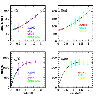
Figure 5: The distance scale $D_{A}(z)$ and $H(z)$ for the fiducial model and the expected measurement errors. The first LRG point is omitted due to coincidence with other data points.

3.2 Constraints on Cosmology – Results from the Fisher Matrix Method

Figure 6: Constraints ($1\sigma$) derived from combing different data sets for a dark energy model with constant equation of state $w$, all assuming the Planck 3-year prior.

Figure 7: Constraints on dark energy parameters $w_{0}$ and $w_{a}$ derived from combining different data sets, all assuming the Planck 3-year prior.

Using the projection method described in §2.1, we derive the error ellipse on the dark energy parameters after marginalizing over other parameters. In Fig. 6, the constraints on a dark energy model of constant equation of state $w$ are plotted for the MAIN1 sample and the combination of the MAIN1, LRG and QSO3 sample. For comparison, we also plot the expected error ellipse from the SDSS LRG sample, which has a good constraint on the dark energy density parameter $\Omega_{X}$ and a poor constraint on $w$. With the LAMOST samples, even for the MAIN1 only sample, there is a significant improvement in constraining $\Omega_{X}$ and $w$. By combining the MAIN1 sample, the LRG sample, and the QSO sample, the allowed range in $w$ is halved with respect to that from the SDSS LRG, reaching a fractional uncertainty of about 6.4%. We did not plot the constraint produced by the MAIN2 sample in the above figure, but it is almost the same as the combination of MAIN1, LRG and QSO3 sample.

Table 4: $~{}w_{0}-w_{a}$ FoM for different samples with $R=1000$ and $R=2000$. The fourth column shows the fractional increasing of FoM by raising the resolution.

Sample/FoM	R=1000	R=2000	+%
MAIN1	5.72	5.79	1.3%
MAIN2	10.83	11.04	1.9 %
LRG	7.94	8.17	2.9%
QSO1	0.554	0.638	15.2%
QSO2	0.903	1.049	16.2 %
QSO3	1.425	1.673	17.4 %

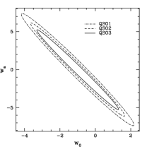
Figure 8: The $1\sigma$ error ellipse for $w_{0}$ and $w_{a}$ for different samples: the main samples (top left), LRGs (top right), QSOs (bottom left), and comparison of main and LRGs (bottom right), all assuming the Planck 3-year prior.

Next we consider the case of evolving equation of state $w$, which is common for dynamical dark energy models. In Fig. 7, we show the constraints on dark energy equation of state parameters from different combinations of the MAIN, the LRG, and the QSO samples. The solid contour shows the dark energy constraints that the LAMOST can achieve with all the samples. There are significant improvements over previous surveys such as the SDSS. However, the constraints on evolving $w$ are still weak, which is in agreement with the assessement of the Dark Energy Task Force (DETF) (Albrecht et al., 2006) that near term projects could not yet provide high precision measurement on $w_{0}$ and $w_{a}$. By combining the BAO measurements with future Type Ia supernovae results, the constraints could be greatly tightened, as shown by the dotted contour in the plot.

In the above we have considered the constraints derived by combining samples of different LAMOST surveys. How much information does each of the samples provide? To address this problem we plot the constraints obtained with each of the samples in Fig. 8. We can see that the galaxy samples provide stronger constraints than the quasar samples, the constraining power of the LRG is between the MAIN1 and MAIN2 samples.

We can also define a Figure of Merit (FoM)

$${\rm FoM}=\frac{1}{\sqrt{\det({{\rm Cov}}(w_{0},w_{a}))}}$$ (28)

which is proportional to the inverse of the contour area. It is 2.01 for the SDSS LRG sample, 5.72 for the MAIN1 sample, 7.94 for the LAMOST LRG sample, 10.83 for the MAIN2 sample. The QSO samples all have very large survey volumes, but due to their low densities, their FoMs are small: ${\rm FoM}_{QSO1}=0.55$, ${\rm FoM}_{QSO2}=0.90$, and ${\rm FoM}_{QSO3}=1.43$. The error ellipses in Fig. 8 reflect this trend: the MAIN2 sample provides the most stringent constraint and the LRG observation could also achieve a similar FoM with much less fiber time. When combining these samples, we reach a FoM of $20.88$. Note that since the MAIN2 sample overlaps the LRG sample, we only include the first two bins of MAIN2 in the combination.

The estimate on the FoMs for galaxy samples is not very sensitive to the adopted value of the bias factors, as long as the constraining power comes mainly from the range of the power spectrum that is not dominated by shot noise (Eq. 8). We test this by adopting observationally inferred bias factor, instead of that from the HOD method. If we ignore the difference in the sample definition and use the bias factors $b=2.35$ (Ross et al., 2007) and $b=1.66$ (Ross et al., 2006) for the LRG sample, we find that the FoM of the LRG sample changes by 1.8% and -6.8%, respectively. For the QSO3 sample, we find that the change in the FoM is 6.9% if the bias factor measured by Porciani et al. (2004) is used in our analysis.

An important question in the design of the surveys is whether to choose $R=1000$ or $R=2000$. With the higher resolution setting, the redshift could in principle be measured to higher precision. However, in practice, for a fixed observation time, a higher signal to noise ratio could be achieved with the lower resolution setting. Conversely, if one requires a fixed signal to noise ratio, more time would be required to complete the survey for the higher resolution setting. For some applications, particularly those on the physics of the galaxies, useful information could be obtained only with the higher resolution setting. For dark energy constraint, the difference between the two choice is largely quantitative. From Fig. 3, we see that there is almost no difference on large scales between the two resolution settings. On small scales, however, the effective volume is larger for the higher resolution setting, which shifts the smearing of small scale power to smaller scales. From the figure, it seems that for galaxy samples the improvement is larger than the QSO samples. However, for the QSO the improvement from the higher resolution occurs at the critical scale of about $0.05\sim 0.1h/{\rm Mpc}$, which is exactly where the baryon oscillation features occur. The figure of merit of dark energy measurement is given in Table 4 for the two settings. For the QSOs, the FoM with $R=2000$ is about $15\%$ bigger than $R=1000$. For the galaxies including both the MAIN and LRG samples, the difference is only a few percent, since the improvement is made largely in the non-linear regime. Therefore, from the perspective of dark energy constraints, $R=1000$ is sufficient and preferred.

3.3 Constraints on Cosmology – Results from the MCMC Method

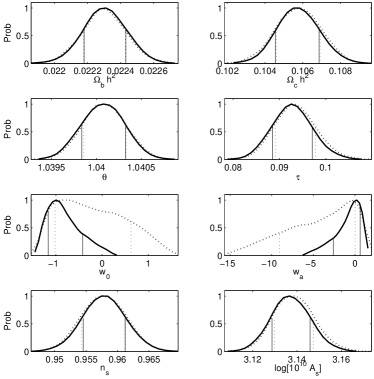
Figure 9: The probability distribution function for some cosmological parameters constrained by combining the CMB and BAO data. The solid and dashed curves correspond LAMOST LRG (MegaZ) sample and the SDSS LRG sample. The 68.3% distribution is marked with two verical lines.

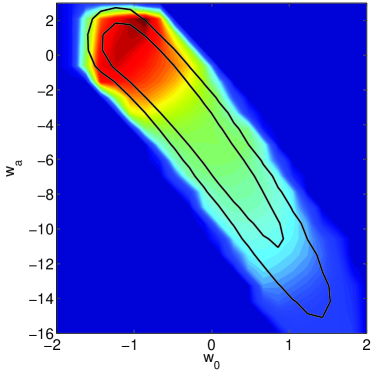
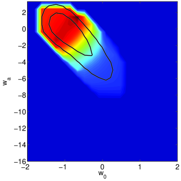
Figure 10: The expected constraints on dark energy equation of state parameters by combining the CMB data and the BAO measurements with the LRG sample. The BAO measurements in the top and bottom panels are assumed to come from the SDSS-II LRG and the LAMOST LRG samples, respectively. Contours in each panel correspond to 68.3% and 95% confidence levels, and the shading shows the mean likelihoods.

We have also performed Monte Carlo simulations for a few cases. In particular we consider the SDSS LRG, which represents our currently available data, and the LAMOST LRG, which represents the precision achievable after two or three years of LAMOST survey. We derive constraints for two cases: (1) only the CMB and BAO data are used; (2) CMB, BAO and SNIa data are used. In the first case, only the “clean” methods (i.e., the CMB and BAO) that are based on well understood physics are used. In the second case, we include a sample of 1200 supernovae expected from SNLS.

In Fig. 9 we show the probability distribution function (PDF) for each of the interested cosmological parameters obtained from the first case after marginalizing over the rest of the parameters. The solid (dashed) curves are from CMB combined with the LAMOST LRG (SDSS-II LRG) sample. Except for those of $w_{0}$ and $w_{a}$, the PDF is well approximated by a Gaussian distribution. There is no significant improvment in the constraints on cosmological parameters other than $w_{0}$ and $w_{a}$ by the addition of the LAMOST data, as the constraints from the CMB data are already very stringent. Compared with the SDSS-II LRG sample, the LAMOST LRG sample helps to significantly tighten the constraints on the dark energy parameters.

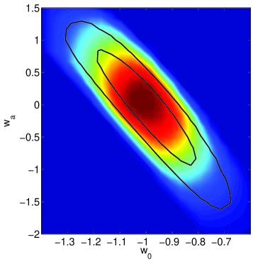
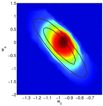
Figure 11: Top: Constraints on $w_{0}$ and $w_{a}$ by combining the CMB (Planck) and the SNIa (SNLS) data. Bottom: Constraints on $w_{0}$ and $w_{a}$ by combining the CMB (Planck), SN Ia (SNLS) and also the BAO (LAMOST LRG) data. Contours correspond to 68.3% and 95% confidence levels, and the shading shows the mean likelihoods.

In Fig. 10 we show the constraints in the $w_{0}$–$w_{a}$ plane. The contours correspond to 68.3% and 95% confidence levels, and the shading is the mean likelihoods of samples (Lewis & Bridle, 2002). With the LAMOST LRGs, the contours are much smaller than those with the SDSS-II LRGs. For our choice of non-linear cut-off scale, the size of the contour generally agrees with the Fisher matrix estimation, but not exactly. In particular, for SDSS-II LRGs, the long tail towards the lower right corner reflects the non-Gaussinity of the likelihood distribution. With only the CMB and BAO data measured by LAMOST, the constraint on dark energy is not very stringent, and many different dark energy model would have easily passed the test.

To improve the constraints on dark energy parameters, we can bring in the SNIa data. To separate the contributions from the SNIa and BAO data, we first show the constraints with CMB and SNIa data in the top panel of Fig. 11. Comparing with the top panel in Fig. 10 (CMB+BAO), we see that the SNIa data provide significant complementary information. The bottom panel of Fig. 11 shows the constraints from all the three data sets (CMB+SNIa+BAO). Compared with CMB+SNIa, adding BAO data from LAMOST LRG further tightens the constraints, increasing the FoM from 33.07 to 42.83. Here, the FoM is defined as $6.17\pi$ over the contour area of 95% confidence level. Such constraints may be able to distinguish some dynamical dark energy models.

4 Conclusion

In this paper we forecast the measurement precision of dark energy equation of state from the BAO measurement expected from LAMOST surveys. We investigate three types of sample targets: magnitude limited surveys of all types of galaxies (main survey), a survey of color-selected luminous red galaxies (LRG), and surveys of quasars (QSO). For the main survey and the QSO survey, we consider a few different magnitude limits, all deeper than the SDSS spectroscopic survey. For the LRGs, we have used the MegaZ sample as our reference sample. The required fiber hours to complete each survey are also estimated (Table2).

For each sample, we predict the redshift distribution, and use the halo model to estimate their clustering bias. We then calculate the effective volume of each survey as a function of wavenumber $k$, the statistical errors in the measured matter power spectrum, and the resulting errors in distance scale measurements with the BAO used as standard rulers. The constraints on the dark energy equation of state parameters are derived using two methods, the Fisher matrix method and the MCMC method.

Our results yield useful insights on how to design the surveys. We find that the MAIN1 sample, which is one magnitude deeper than the SDSS main sample has an effective volume about three and half times larger than the SDSS main sample. Similarly, with the LAMOST LRGs, an effective volume of about four times of the SDSS LRG can be obtained. This effective volume is almost as large as the much more time-consuming MAIN2 sample (two magnitudes deeper than the SDSS main sample). The QSO samples can also yield high effective volume at large scales, but it declines rapidly at small scales. The improvement on the measurement of dark energy equation of state depends not only on the large scale effective volume, but also on the effective volume at relatively small scales. Our investigation shows that although the effective volume of the LAMOST LRG sample is comparable to the MAIN2 at large scales, the latter’s figure of merit for dark energy measurement is greater. The QSO sample, on the other hand, generally has lower figure of merit. However, the number of targets and required observing fiber hours of the QSO samples are also much smaller than the galaxy samples, so it should not be regarded as a competing project of the galaxy surveys. The efficient design for using LAMOST survey to constrain dark energy parameters is to have a MAIN1 survey, an LRG survey supplemented by a QSO survey.

We also studied the impact of spectral resolution. The figure of merit improves by only about 1%-3% for the galaxy samples when one switches the spectral resolution from 1000 to 2000. For quasars the figure of merit improvement is about 15%. From the point of view of dark energy constraints, it is unnecessary to achieve a high spectral resolution, although high resolution spectra are useful for other scientific objectives.

Finally, we also used Monte Carlo simulations to make the same forecast to test the accracy of the Fisher matrix result. The figure of merits of the two estimate roughly agree, although the contours obtained from the Monte Carlo method are not exactly ellipses, but rather asymmetric.

Overall, the LAMOST surveys could achieve an figure of merit (as defined by Wang (2008)) of 5-10 from each individual galaxy samples. For a constant $w$ dark energy model, the expected precision on $w$ is about 6.9%. For time-dependent $w$ models, the LAMOST survey would also help to significantly improve the constraints on the equation-of-state parameters, although the expected errors on $w_{0}$ and $w_{a}$ are not tight enough to pin down the nature of dark energy.

Appendix A The LAMOST telescope

The LAMOST telescope (see e.g., Chu 1998; Stone 2008) is a 4 meter telescope, its design features an fixed horizontal meridian reflecting Schmidt configuration, with an active Schimidt correcting plate to achieve both wide field of view ($5\degr$ diameter, or $20\deg^{2}$) and large aperture. The focal plane accommodates 4000 optical fibers for spectrographic observations. The optical axis is fixed in the meridian plane, taking measurements of targets as they pass through the meridian (typically a target can be tracked for about 2 hours.) The telescope is located at the Xinglong station ($117\degr 34\arcmin 30\arcsec$ East, $40\degr 23\arcmin 36\arcsec$ North) of the National Astronomical Observatory of China, and can observe the part of sky with declination $-10\degr<\delta<90\degr$. The construction of the LAMOST telescope was completed by August 2008 and it is undergoing engineering tests and calibrations. The surveys are expected to begin in 2010/2011 and last for at least 5 years.

The LAMOST is to be equipped with both low resolution spectrographs and medium resolution spectrographs (Zhu & Xu, 2000; Zhu et al., 2004), the latter is used mainly for bright targets such as stars. For extragalactic observations using the low resolution spectrographs, spectra can be taken with two resolution settings: (1) using the full sized fiber, the resolution is 1000 (2) using half sized fiber, the resolution is 2000. The main features of the telescope is summarized in Table 5.

The LAMOST has a parallely controlled fiber positioning system with 4000 optical fibers(Xu, 2003; Zhu et al., 2004), each individually driven by two micro-stepping motors and can move within a circle of 30 mm diameter (corresponding to $340\arcmin$ on the sky) to aim at a target within the circle. The distance between two adjacent circle axes are 26 mm, slightly smaller than the diameter of the circle, so that adjacent circles overlap. This allows full coverage of the focal plane. Due to fiber collision, targets within 55 arcsec can not be observed at the same time. The average angular density of the fibers is about 200 per square degree. The whole assembly is controlled by computer and can be adjusted in real time. Acquiring new target and adjust the fibers takes a few minutes typically.

As the LAMOST telescope is dedicated to spectroscopy and does not have imaging capability, photometric catalogue compiled from other surveys would be used to select targets. The LAMOST will carry out several different survey projects simultaneously. The input catalogue of these different surveys will be combined (with different assigned priority) to produce the general input catalogue of LAMOST. A software system (Peng et al., 2004) would then select targets of observation from this catalogue, taken into account the priority of the target, the observing time and target area, the lunar phase and weather condition etc, this allows more efficient use of the fibers and observing time. During each run, the selected targets are a mixture of different survey projects, so the appropriate measure of observing resource is the fiber time, i.e. the number of fibers allocated multiplied by the observing time.

Table 5: Main Characteristics of LAMOST

Average aperture	4 m
Field of view	$5\,^{\degr}$
Focal plane	$\phi 1.75$m
Focal length	20 m
Number of fibers	4000
Spectral ranges	370-900nm
Spectral resolution	1000 or 2000
Minimal distance of adjacent targets:	$55\arcmin$
Observable sky	$-10\,^{\degr}<\delta<+90\,^{\circ}$

The collecting area of LAMOST is about 2.2 times that of the SDSS telescope, which has an aperture of 2.7m. We would expect that for comparable exposure time, target of one magnitude deeper could be observed if the system efficiency and sky background are the same. The system effeciency, in turn, also depends on the positioning error of the fiber. The signal to noise ratio of an observation with different conditions and parameters has been estimated using ray tracing method, and a calculator has been developed for estimation (Xue, 2008). For the present paper, we assume an average fiber positioning error of $0.5\arcsec$, and a sky background of 20.5 in r band . We also assume that an average signal to noise ratio of 4 per spectral resolution pixel is achieved for both galaxies and point sources. This is about the minimum for redshift measurement. Surveys with low signal to noise ratio allows fast survey of a large number of targets, however, in the real survey, a higher signal to noise ratio may be required for other scientific purposes.

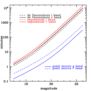
Figure 12: Expected exposure time of different bands and model profiles, assuming spectral resolution 1000, S/N=4 per spectral pixel, a sky background of 20.5 in the respective band (r or i), fiber positioning error $0.5\arcsec$, $r_{e}=3\arcsec$ for exponential profile and $r_{e}=4\arcsec$ for de Vaucouleurs profile.

The required exposure time for achieving the desirable signal to noise ratio depends also on the size of the object (characterized by the half-light radii of the image $r_{50}$ for extended source), the seeing of the sky, and the point spread function of the optical system. We characterize the angular size of the target by a parameter $r_{e}$. For the de Vaucouleurs profile which represents elliptical galaxies,

$$I_{\rm deV}(r)=I_{0}\exp{[-7.67(r/r_{e})^{1/4}]},$$

and for the exponential profile which represents spiral galaxies,

$$I_{\exp}(r)=I_{0}\exp{[-1.68r/r_{e}]}.$$

Analysis of the half-light radii ($r_{50}$) of SDSS galaxies show that (Blanton et al., 2001) about 80% galaxies have $r_{50,petro}\leq 3\arcsec$. For the exponential profile $r_{50,petro}=r_{50,true}=r_{e}$, and for the de Vaucouleurs profile, $r_{50,petro}\approx 0.7r_{50,true}=0.7r_{e}$. Thus, for a simple estimate of the size of the targets, we assume that the average target has $r_{e}=3\arcsec$ and $4\arcsec$ for exponential profile and de Vaucouleurs respectively.

In Fig. 12, we plot the exposure time required for targets of different sizes, bands and model profiles. As can be seen from the figure, for a given S/N, the integration time is proportional to $f^{-1}$ for bright sources, where $f$ is the flux, and to $f^{-2}$ for the faint sources where the sky background noise dominates. Compared with elliptical galaxies, the spiral typically requires more time for observation to reach the same magnitude, this comprises about 25% - 50% of our sample. Observing large samples of targets fainter than $r=21$ would be impractical.

The spectral resolution of the low-resolution grating is 1000 when the full sized fiber is used, 2000 when half sized fiber is used. When observing a galaxy or quasar with multiple lines, the redshift could be measured with accuracy better than the grating resolution if multiple spectral lines are present and the signal to noise ratio is high. However, the number of usable lines may be limited for many galaxies, and to save observing time the signal to noise ratio is perhaps not very high in large scale observations, so we assume the redshift measurement precision to be 1/1000 or 1/2000.

Appendix B Design of the extragalactic surveys

Since the LAMOST does not have imaging capability by itself, the targets of the spectroscopic survey must be selected from photometric catalogues compiled from observational data obtained by other instruments. At present, the SDSS photometric catalogue is the largest of such catalogue, which covers about $8000\deg^{2}$ of northern sky up to $r=23$, and only a small fraction of the objects on this catalogue has been targeted by the SDSS spectroscopic surveys. One may also consider to conduct a photometric survey for a part of the south galactic cap to supplement this. Regions of low galactic latitude are of less interest for extragalactic surveys due to the higher extinction. In the future more targets could be obtained from photometric surveys which are being planned, e.g., the Pan-Starrs surveys. However, as discussed in Appendix A, it is unlikely for LAMOST to observe a large number of very faint objects within the limited observation time available.

In the present work, we shall consider three surveys: (1) a magnitude limited general survey of galaxies of all types which we shall call the main survey; (2) an LRG survey; (3) a magnitude limited low redshift $(z<2.1)$ quasar survey. In Table  2 we list a summary of these surveys, including the surface density, total number of targets, and required fiber hours.

B.1 The main survey

In the original feasibility study of the LAMOST, a typical number quoted is B=20.5 for an exposure time of 1 hour, this is comparable to the present estimate. The SDSS team has chosen their main sample using an r-band limit, as the r-band luminosity is a better tracer for mass. Here we assume the survey limit is given in r-band. The magnitude limit we quote here is just a strawman value and can be changed for the real survey. It is reasonable to consider a sample which is one or two magnitudes deeper than the SDSS main sample. The SDSS main sample has a magnitude limit of r=17.77, the exposure time is typically about 45 minutes (Strauss et al., 2003). We consider two samples: a magnitude limited sample which is one magnitude deeper than the SDSS main sample, i.e. $r<18.8$ (hereafter MAIN1), and also a sample which is 2 magnitudes deeper than SDSS main, i.e. $r<19.8$ (hereafter MAIN2).

Given the above magnitude limit, we may estimate the angular density of targets using galaxies number count (Yasuda et al., 2001) or the observed luminosity function (Blanton et al., 2003). Yasuda et al. (2001) have shown that the observed number of galaxies $N(m)$ can be well fitted by assuming the Euclidean geometry for three-dimensional space, which gives the number of galaxies brighter than $m$

$$N(m)\propto 10^{0.6m}$$ (29)

Alternatively, the luminosity function of SDSS galaxies was given in Blanton et al. (2003)

$$\Phi(M,z)=0.4\ln{10}\times\Phi^{\star}10^{0.4(\alpha+1)(M^{\star}-M)}\exp(-10^{0.4(M^{\star}-M)})$$ (30)

and the redshift evolution of the luminosity is modelled by

$$\Phi^{\star}(z) = \Phi^{\star}(z_{0})10^{0.4P(z-z_{0})}$$ (31)

$$M^{\star}(z) = M^{\star}(z_{0})-Q(z-z_{0})$$ (32)

The absolute magnitude $M$ is related to the apparent magnitude $m$ and redshift z as

$$M-5\log_{10}h=m-DM(z)-K(z)$$ (33)

where $DM(z)$ is the distance modulus and $K(z)$ the K-correction. The K-correction depends on the SED of the galaxy, we have adopted a simple approximation of $K(z)\approx-0.21+1.1z$, which is approximately the median K-correction for the 12 types of galaxy SEDs given in Blanton et al. (2003). This may not be very accurate for individual galaxies, but should suffice for the purpose of estimating the angular density.

Figure 13: The angular density of objects as a function of limiting magnitude in the general galaxy survey. The solid line corresponds to the (apparent) magnitude integration of the galaxies number count (Yasuda et al., 2001) at SDSS commission stage. The dashed line is the result of (absolute) magnitude-spatial integration of the luminosity function (Blanton et al., 2003), by using the best-fitted $r$ band evolution parameter $Q=1.62,~{}P=0.18$ and a simple K correction model.

We show in Fig. 13 the integrated angular density as a function of the magnitude limit in $r$ band. The solid curve is obtained by using the galaxies number count given in Yasuda et al. (2001), and the dashed curve is obtained by using the luminosity function of Blanton et al. (2003). These data have to be extrapolated to faint end or high redshift to obtain the distribution function. We use the best-fitted $r$ band evolution parameter $Q=1.62,~{}P=0.18$ given in Blanton et al. (2003). In this paper, we have used the number count directly for the fibre time estimation, but for cosmological constraints we used the luminosity function. There is only slight difference between these two.

For the MAIN1 ($r=18.8$) sample, the angular density is $330\deg^{-2}$, about 1.65 times the average angular density of the fibers. Most targets can be observed in one to two observing runs (due to fiber collision, there could be a small fraction which is left unobserved). For MAIN2, the angular density is about $1050\deg^{-2}$. These can be observed in 5-6 observing runs.

The total number of target is about 2.6 million for the MAIN1 survey, and 8.4 million for the MAIN2 survey. The total fiber time required for completing the survey is about 0.88 million fiber hours for MAIN1, and 14 million fiber hours for MAIN2. If we assume that all fibers are allocated for this survey, and for each night the observing time is 6 hours, then MAIN1 observation can be completed in 37 clear dark (moonless) nights, and MAIN2 in 584 clear dark nights. In reality, the automatic survey strategy system will probably assign targets of different surveys in the same sky area at the same time, and only 1/3-1/2 of the nights have good weather. Thus, we expect that the MAIN1 sample can be surveyed in the first year, while the MAIN2 sample in the next 5-10 years, depending on the weather condition and the fraction of fiber time allocated for this survey .

Table 6: HOD parameters for galaxies (reproduced from Zehavi et al. (2005b)).

$M^{\rm max}_{r}$	$\log_{10}m_{min}$	$\log_{10}m_{1}$	$\alpha$
-22.0	13.91	14.92	1.43
-21.5	13.27	14.60	1.94
-21.0	12.72	14.09	1.39
-20.5	12.30	13.67	1.21
-20.0	12.01	13.42	1.16
-19.5	11.76	13.15	1.13
-19.0	11.59	12.94	1.08
-18.5	11.44	12.77	1.01
-18.0	11.27	12.57	0.92

Figure 14: The clustering bias of the main sample as a function of redshift. Curves from the top down correspond to the magnitude limit of 17.8, 18.3, 18.8, 19.2, 19.8.

We can estimate the bias of the main sample using the halo model as outlined in §2.3. The HOD parameter for all galaxy types have been measured for the SDSS main sample DR2 (Zehavi et al., 2005b), which consists of 204,584 galaxies over $2,947\deg^{2}$ with apparent luminosity $10.5<r<17.77$ and redshifts extended to $z\sim 0.2$. The mean number of galaxies above limiting luminosity $L_{lim}$ in halos of mass $m$ is parameterized as

$$\langle N(m,L>L_{lim})\rangle=\Theta(m-m_{\rm min})[1+(m/m_{1})^{\alpha}],$$ (34)

where $\Theta(x)$ is the Heaviside step function, and the HOD parameters $\theta\equiv\{m_{min},m_{1},\alpha\}$ are all functions of the limiting luminosity $L_{lim}$ and redshift $z$, their measured values are given in Table 3 of Zehavi et al. (2005b). However, Zehavi et al. (2005b) gives only the measured value at $z_{m}\sim 0.1$, at higher redshift the data is not available. Since the LAMOST galaxy sample would have much higher average redshift, evolution of HOD parameters should be considered. We have adopted the simple ansatz that the HOD parameters are functions of one parameter $\lambda$ only, $\lambda$ is a function of both the actual limiting luminosity $L$ and the redshift $z$. At $z=z_{m}$, $\lambda(L,z_{m})=L$, and $\theta[\lambda(L,z)]=\theta(L,z_{m})$ as given in Zehavi et al. (2005b). With this ansatz, in order to know $\theta(L,z)$ at a higher $z$, we only need to know the corresponding $\lambda(L,z)$. To obtain $\lambda$, we calculate the galaxy density at $z$ using the HOD parameters obtained with a trial value of $\lambda$, compare it with the density integrated from the measured luminosity function $\phi(L,z)$ given in Blanton et al. (2003),

$$\int_{0}^{\infty}dm\frac{dn}{dm}\langle N(m,L>L_{lim},\lambda)\rangle=\int_{L_{lim}}^{\infty}\phi(L,z)dL,$$ (35)

where $\langle N(m,L>L_{lim},\lambda)\rangle$ is given in eq. 34. The value of $\lambda$ is adjusted so that the galaxy densities calculated with the HOD matches the observation. Of course, this ansatz may not be true. However, since we match the luminosity function at different redshifts, the estimate of bias would not be too far off.

By using this method, we obtain an estimate of the bias at different redshifts. For example, for the MAIN1 sample, at $z=0.1$, the bias is $b=1.0$, and at $z=0.3$, $b=1.44$. For the MAIN2 sample, $b=0.92$ at $z=0.1$, $b=1.14$ at $z=0.3$, and $b=1.66$ at $z=0.5$. The bias as a function redshift is plotted in Fig. 14. For reference, besides the $r=18.8$ and $19.8$ main survey samples, we also plotted several samples of different magnitude limits.

The distributions of galaxies as a function of redshift are plotted in Fig. 1. The MAIN1 sample peaks at $z\sim 0.2$, but extends beyond $z=0.4$, where comoving number density decrease to $n(z=0.4)\approx 7\times 10^{-5}(h/{\rm Mpc})^{3}$. The MAIN2 sample has a more extended distribution, up to $z=0.6$ with the same cut-off density. The corresponding comoving density distributions are plotted in Fig. 15.

B.2 The LRG survey

The LRGs are intrinsically brighter and can be selected by their colors. At present, a catalogue of LRGs have already been compiled from the SDSS photometric data, namely the MegaZ LRG catalogue (Collister et. al., 2006). This is a catalogue of LRG galaxies selected from the SDSS DR4 imaging data, which covers $5914\deg^{2}$, with $17.5<i_{dev}<20.0$. The total number of galaxies in this catalogue is 1.2 million, and photometric redshifts for these galaxies have been obtained, with an error of $\sigma_{z}=0.048$. It is expected that the sample will be extended to $8000\deg^{2}$, and a total number of 1.5 million of LRGs. The sample selection of LRGs might be further tailored for the needs of LAMOST, nevertheless it should have a lot in common with the MegaZ sample, particularly at $z>0.4$. We therefore tentatively take the properties of this sample as the LAMOST LRG survey sample in our estimation.

We expect that an exposure time of at least 70 minutes is required for observing most of these targets. The angular density of the sample is about 205 per square degree, which is very close to the angular number density of the fibers of LAMOST (200). The total observing fiber time required for completing 8000 square degree area is about 1.9 million fiber hours (80 nights).

Note that there is not a unique selection criterion of LRGs, hence the LRGs in the MegaZ sample may differ slightly from those already spectroscopically observed in the SDSS-II, or those observed in the 2SLAQ survey (Cannon et al., 2006). The color cut used by MegaZ is similar to but somewhat broader than that used by 2SLAQ. It includes bluer objects, which is in turn bluer than the Cut II of SDSS LRG to accommodate the higher density of 2dF fibers. Wake et al. (2006) has compared the selection criterion difference between SDSS and 2SLAQ for the evolution of luminosity function, they started from SDSS main sample which consists of all galaxies with $r<17.77$, then evolved these to $z=0.2$ (for SDSS) and $z=0.55$ (for 2SLAQ) by interpolating between passive and continous star formation model according to the observed $g-i$ color. They found that 90% of the SDSS LRG would be selected by 2SLAQ, while only 30% of the 2SLAQ LRG would be selected by SDSS. The number distribution of the MegaZ sample (marked LAMOST LRG) is shown in Fig. 1, most targets in this catalogue have redshifts between 0.4 and 0.7. It peaks aroud $z=0.45$. Nearly 20% of the objects in the catalogue (Collister et. al., 2006) are located within the region with $0.50<d_{\perp}<0.55,~{}d_{\perp}=(r-i)-(g-r)/8.0$. If these objects are removed, then the photometric redshift distributions of the MegaZ-LRG catalogue and the 2SLAQ evaluation set would become similar (c.f. Figure. 12 in Collister et. al. (2006)).

To estimate the bias of the Mega-Z sample, we use the HOD parameters for red galaxies as given in Brown et al. (2008), which is obtained by using the observed luminosity function and the luminosity-dependent clustering of 40696 red galaxies with $0.2<z<1.0$. The HOD parameters can be approximated as a function of redshift and B-band absolute magnitude $M_{B}+1.2z$, which is an effective proxy for stellar mass:

$$M_{min}(h_{-1}M_{\odot})=10^{11.95}\times 10^{0.4\times[-19-(M_{B}-5\log h+1.2z)]}$$

$$+10^{13.70}\times 10^{1.15\times[-21-(M_{B}-5\log h+1.2z)]}+10^{11.85}$$ (36)

$$M^{{}^{\prime}}_{1}(h_{-}1M_{\odot})=10^{12.70}\times 10^{0.11\times[-17-(M_{B}-5\log h+1.2z)]}$$

$$+10^{14.60}\times 10^{0.85\times[-21-(M_{B}-5\log h+1.2z)]}$$ (37)

with $M_{0}=M_{min}$, $\sigma_{\log M}=0.3$ and $\alpha=1$. Since the bands are different and the transformation between them are complicated, again, we calculate the bias by tuning the B band magnitude threshold to match the space density, then use the formalism presented in §2.3. We find the biases of the sample are 1.77 at z=0.475, and 2.29 at z=0.625.

Table 7: Bias

MegaZ		MAIN1		MAIN2
z	$b_{g}$	z	$b_{g}$	z	$b_{g}$
0.475	1.77	0.10	1.00	0.1	0.92
0.625	2.29	0.3	1.44	0.3	1.14
				0.5	1.66
QSO1		QSO2		QSO3
z	$b_{g}$	z	$b_{g}$	z	$b_{g}$
0.575	1.26	0.530	1.23	0.53	1.24
0.885	1.57	0.790	1.41	0.80	1.42
1.155	1.92	1.068	1.72	1.07	1.62
1.425	2.32	1.363	2.11	1.35	1.96
1.695	2.77	1.658	2.55	1.65	2.36
1.965	3.26	1.953	3.04	1.95	2.79

Figure 15: The comoving number density of galaxy samples.

B.3 QSO survey

Finally, we consider a QSO survey. The Ly$\alpha$ forest of the QSO can be a powerful probe of the baryon acoustic oscillation (McDonald & Eisenstein, 2007), but here the QSO itself is used as tracers. In past surveys such as the 2dF and SDSS, the low number density of QSOs prevents it from being a good tracer target for measuring BAO features. However, with LAMOST the comoving number density can be greater, making it more useful for such purpose. Using the 2SLAQ sample (Richards et al., 2005), which consists of 5645 quasars down to $g=21.85$ in 105.7 deg², we obtain a luminosity function of the quasars. Unlike the Schechter form of galaxies luminosity function, the QSO luminosity function is modelled as a double power law (Croom et al., 2004; Richards et al., 2005)

$$\Phi(M_{g},z)=\frac{\Phi^{*}}{10^{0.4(\alpha+1)(M_{g}-M_{g}^{*})}+10^{0.4(\beta+1)(M_{g}-M_{g}^{*})}}$$ (38)

For estimation we assume here that the evolution with redshift is pure luminosity evolution, individual quasars is fainter today than at z = 2, with the dependence of the characteristic luminosity described by (Richards et al., 2005)

$$M_{g}^{*}(z)=M_{g}^{*}-2.5(k_{1}z+k_{2}z^{2})$$ (39)

where $\alpha=-3.28,~{}\beta=-1.78,~{}M^{*}=-22.68,~{}k_{1}=1.37,~{}k_{2}=-0.32,~{}\Phi^{*}=5.96\times 10^{-7}{\rm Mpc}^{-3}$. In reality, the evolution of quasar luminosity function may be due to a combination of decreasing space density and decreasing luminosity of individual quasars, but this would not significantly affect our result. We calculated the QSO K-correction by assuming that the continuum $F_{\nu}\propto\nu^{-0.5}$.

The quasar number density is plotted in Fig. 16. Consider samples with the magnitude limits, $g<20.5$ (QSO1), $g<21.0$ (QSO2), and $g<21.65$ (QSO3), all between $z=0.4$ and $z=2.1$. The density of these magnitude limited samples drops at low redshift, because there is a lower limit $M_{g}<-22.5$ on the absolute luminosity for quasars (this also reflects a decrease in quasar activity at low redshifts). The turning redshift $z_{t}$ is the place where $M_{g}(z_{t},m_{g,lim})=M_{g,lim}$, and $M_{g,lim}=-22.5$. They are $z_{t,QSO1}=0.75,~{}z_{t,QSO2}=0.92,~{}z_{t,QSO3}=1.20$.

Figure 16: Comoving number density of the QSO samples with QSO1 ($g<20.5$), QSO2 ($g<21.0$) and QSO3 ($g<21.65$).

The angular density of the QSO1 is $30\deg^{-2}$, and the total number is 0.24 million for 8000 $\deg^{2}$. The observing time is about 15 minutes for signal-to-noise ratio $S/N=4$, so it requires about 0.06 million fiber hours. For QSO2 sample, the angular density is $45\deg^{-2}$, the spectrum can be obtained within 30 minutes for the same S/N, and requires 0.18 million fiber hours. The angular density of QSO3 is $72\deg^{-2}$, the required integration time is 1.5 hours, depending on the sky background. It needs 0.855 million fiber hours to complete the survey.

The bias of a QSO sample can be estimated using the method given in §2.3. Alternatively, it can also be measured directly from the projected two point correlation function. Porciani et al. (2004) made an measurement with about 14,000 quasars at $0.8<z<2.1$ in the 2dF/6dF QSO Redshift Survey. They found a slightly greater bias (see Table. 7) than that of the estimate obtained using the method of §2.3. The difference is greater at higher redshifts (10% at $z=1.5$, and 25% at $z=1.9$) (Marulli et al., 2006). Our estimate may be improved by using more detailed semi-analytical models, but for our purpose this simple estimate should suffice.

References

- Abdalla & Rawlings (2005) Abdalla, F. B., Rawlings, S., 2005, MNRAS, 360, 27.
- Albrecht et al. (2006) Albrecht, A. et al. (Dark Energy Task Force), arxiv:astro-ph/0609591
- Alcock & Paczynski (1979) Alcock, C., Paczynski, B., 1979, Nature, 281, 358.
- Angulo et al. (2008) Angulo, R., Baugh, C., M., Frenk, C., S., and Lacey, C., G., 2008, MNRAS, 383, 755.
- Astier et al. (2006) P. Astier et al., 2006, A&A, 447, 31.
- Bassett et al. (2005) Bassett, B. A., Nichol, R. C., Eisenstein, D. J., 2005, A&G., 46, 26.
- Berlind & Weinberg (2002) Berlind, A. A., & Weinberg, D. H., 2002, ApJ, 575, 587.
- Blake & Glazebrook (2003) Blake, C., Glazebrook, K., 2003, ApJ, 594, 665.
- Blake et al. (2006) Blake, C., Parkinson, D., Bassett, B., Glazebrook, K., Kunz, M., Nichol, R. C., 2005, MNRAS, 365, 255.
- Blake, Collister & Lahav (2007) Blake, C., Collister & A., Lahav, O., 2007, arxiv:0704.3377.
- Blanton et al. (2001) Blanton, M. R., Dalcanton, J., Eisenstein, D., Loveday, J., Strauss, M. A., SubbaRao, M., Weinberg, D. H., 2001, AJ, 121, 2358.
- Blanton et al. (2003) Blanton, M. R.et al. 2003, AJ, 592, 819.
- Brown et al. (2008) Brown, M., Zheng, Z., White, M., Dey, A., Jannuzi, B. T. Benson, A. J., Brand K., Brodwin, M., Croton, D. J., 2008, arxiv:0804.2293
- Brown et al. (2003) Brown, M. J. I., Dey, A., Jannuzi, B. T., Lauer, T. R., Tiede, G. P., Mikles, V. J., 2003, ApJ, 597, 225.
- Cabre&Gaztanaga (2008a) Cabre, A., Gaztanaga, E., arXiv:0807.2460 [astro-ph].
- Cabre&Gaztanaga (2008b) Cabre, A., Gaztanaga, E., arXiv:0807.2461 [astro-ph].
- Cannon et al. (2006) Cannon, R.,et al., 2006, MNRAS, 372, 425.
- Chu (1998) Chu, Y., 1998, Highlights of Astronomy, 11A., 493.
- Cimatti et al. (2008) Cimatti, A., Robberto, M., Baugh, C.M., Beckwith, S.V.W., Content, R., Daddi, E. De Lucia, G., Garilli, B., Guzzo, L., Kauffmann, G., Lehnert, M., Maccagni, D., Martinez-Sansigre, A., Pasian, F., Reid, I.N., Rosati, P., Salvaterra, R., Stiavelli, M., Wang, Y., Zapatero Osorio, M., (SPACE team), arxiv:0804.4433.
- Coil et al. (2005) Coil, A. L., Newman, J. A., Cooper, M. C., Davis, M., Faber, S. M., Koo, D. C., Willmer, C. N. A., 2006, ApJ, 644, 671.
- Cole et al. (2005) Cole, S. et al. (2dFGRS team), 2005, MNRAS, 362, 505.
- Collister & Lahav (2005) Collister, A. A., & Lahav, O., 2005, MNRAS, 361, 415.
- Collister et. al. (2006) Collister, A. et al., 2007, MNRAS 375, 68.
- Cooray & Sheth (2002) Cooray, A., Sheth, R. K., 2002, Phys. Rept., 372, 1.
- Crocce & Scoccimarro (2006a) Crocce, M., Scoccimarro, R., 2006, PRD, 73, 063519.
- Crocce & Scoccimarro (2006b) Crocce, M., Scoccimarro, R., 2006, PRD, 73, 063520.
- Crocce & Scoccimarro (2007) Crocce, M., Scoccimarro, R., 2008, PRD, 77, 023533.
- Croom et al. (2004) Croom, S. M., Smith, R. J., Boyle, B. J., Shanks, T., Miller, L., Outram, P. J., Loaring, N. S., 2004, MNRAS, 349, 1397.
- Eisenstein et al. (1997) Eisenstein, D. J., Hu, W., Silk, J., Szalay, A. S., 1998, ApJ, 494, L1.
- Eisenstein & Hu (1998) Eisenstein, D. J., Hu, W., 1998, ApJ, 496, 605.
- Eisenstein, Hu & Tegmark (1999) Eisenstein, D. J., Hu, W., Tegmark, M., 1999, ApJ, 518, 2.
- Eisenstein et al. (2001) Eisenstein, D. J. et al., 2001, AJ, 122, 2267.
- Eisenstein & White (2004) Eisenstein, D. J. & White, M. J., 2004, PRD, 70, 103523.
- Eisenstein (2005a) Eisenstein, D. J., 2005, New Astronomy Reviews, 49, 360.
- Eisenstein (2005b) Eisenstein, D. J. et al., 2005, ApJ, 633, 560.
- Eisenstein,Seo&White (2006) Eisenstein, D. J., Seo H, J., White, M. J., 2007, ApJ, 664, 660.
- Feldman, Kaiser &Peacock (1994) Feldman, H. A., Kaiser, N., Peacock, J. A., 1994, ApJ, 426, 23.
- Feng, Chu, & Yang (2000) Feng, L.-L., Chu, Y.-Q., Yang, Y.-H., 2000, ChA&A, 24, 413
- Glazebrook & Blake (2005) Glazebrook, K. & Blake, C., 2005, ApJ, 631, 1.
- Glazebrook et al. (2007) Glazebrook, K., et al., 2007, arxiv:astro-ph/0701876.
- Guzik & Bernstein (2007) Guzik, J. & Bernstein, G., 2007, MNRAS 375, 1329.
- Hu & White (1996) Hu, W. & White, M. J., 1996, ApJ, 471, 30.
- Hutsi (2005a) Hutsi, G., 2005, arxiv:astro-ph/0507678.
- Huetsi (2005b) Huetsi, G., 2005, A&A, 449, 891.
- Jing et al. (1998) Jing, Y. P., Mo, H. J., Borner, G., 1998, ApJ, 494, 1.
- Kaiser (1987) Kaiser, N., 1987, MNRAS 227, 1.
- Kamionkowski et al. (1996) Kamionkowski, M., Kosowsky, A., Stebbins, A., 1997, PRL, 78, 2058.
- Koehler et al. (2007) Koehler, R. S., Schuecker, P., Gebhardt, K., 2007, A&A, 462, 7.
- Lacey & Cole (1993) Lacey, C. G. & Cole, S., 1993, MNRAS, 262, 627.
- Lewis & Bridle (2002) Lewis, A. & Bridle, S., 2002, PRD, 66, 103511.
- Li et al. (2008) Li, H., Xia, J. Q., Fan, Z., Zhang, X., 2008, arxiv:0806.1842
- Linder (2003) Linder, E. V., 2003, PRD, 68, 083504.
- Magliocchetti & Porciani (2003) Magliocchetti, M. & Porciani, C., 2003, MNRAS 346, 186.
- Marulli et al. (2006) Marulli, F., Crociani, D., Volonteri, M., Branchini, E., Moscardini, L., 2006, MNRAS, 368, 1269.
- Matsubara & Szalay (2003) Matsubara, T., Szalay, A.S., 2003, PRL 90, 021302.
- Meiksin et. al (1999) Meiksin, A., White, M. J., Peacock, J. A., 1999, MNRAS, 304, 851.
- McDonald et al. (2006) McDonald, P., et al., 2006, ApJS, 163, 80.
- McDonald & Eisenstein (2007) McDonald, P., Eisenstein, D., 2007, PRD, 76, 063009.
- Okumura et al. (2008) Okumura, T., Matsubara, T., Eisenstein, D. J., Kayo, I., Hikage, C., Szalay, A. S., Schneider, D. P., 2008, ApJ, 676, 889.
- Padmanabhan et al. (2008) Padmanabhan, N., White, M., Norberg, P., Porciani, C., 2008, arxiv:0802.2105.
- Peacock (2000) Peacock, J. A., Smith, R. E., 2000, MNRAS, 318, 1144.
- Peng et al. (2004) Peng, X. B., Xing, X. Z., Hu, H. Z., Zhai, C., Li, W. M., 2004, in Advanced Software, Control, and Communication Systems for Astronomy, Proc. SPIE 5496, 497.
- Percival et al. (2007) Percival, W. J., Cole, S., Eisenstein, D. J., Nichol, R. C., Peacock, J. A., Pope, A. C., Szalay, A. S., 2007, MNRAS, 381, 1053.
- Perotto et al. (2006) Perotto, L., Lesgourgues, J., Hannestad, S., Tu, H., Wong, Y. Y. Y., 2006, JCAP, 0610, 013.
- Peterson, Bandura & Pen (2006) Peterson, J.B., Bandura, K., Pen, U. L., 2006, arxiv:astro-ph/0606104
- Planck Collaboration (2006) Planck Collaboration, 2006, arxiv:astro-ph/0604069.
- Phleps et al. (2006) Phleps, S., Peacock, J. A., Meisenheimer, K., Wolf, C., 2006, A&A, 457, 145.
- Porciani et al. (2004) Porciani, C., Magliocchetti, M., Norberg, P., 2004, MNRAS, 355, 1010.
- Press & Schechter (1974) Press, W. H., Schechter, P., 1974, ApJ, 187, 425.
- Richards et al. (2005) Richards, G. T., et al.,2005, MNRAS, 360, 825.
- Ross et al. (2006) Ross, N. P., et al., 2007, MNRAS, 381, 573.
- Ross et al. (2007) Ross, N. P., Shanks, T., Cannon, R. D., Wake, D. A., Sharp, R. G., Croom, S. M., Peacock, J. A., 2008, MNRAS, 387, 1323.
- Schneider et al. (2005) Schneider, D. P., et al., 2005, AJ, 130, 367.
- Schneider et al. (2007) Schneider, D. P., et al., 2007, AJ, 134, 102.
- Scoccimarro et al. (2001) Scoccimarro, R., Sheth, R. K., Hui, L., Jain, B., 2001, ApJ, 546, 20.
- Seljak & Zaldarriaga (1996) Seljak, U., Zaldarriaga, M., 1996, ApJ, 469, 437.
- Seljak (1997) Seljak, U., 1997, ApJ, 482, 6.
- Seljak (2000) Seljak, U., 2000, MNRAS, 318, 203.
- Seo & Eisenstein (2003) Seo, H. J., Eisenstein, D. J., 2003, ApJ, 598, 720.
- Seo & Eisenstein (2007) Seo, H. J., Eisenstein, D. J., 2007, ApJ, 665, 14.
- Seo et al. (2008) Seo, H. J., Siegel, E. R., Eisenstein, D. J., and White, M., 2008, ApJ, 686, 13.
- Sheth & Tormen (1999) Sheth, R. K., Tormen, G., 1999, MNRAS, 308, 119.
- Sheth (2001) Sheth, R. K., Diaferio, A., 2001, MNRAS, 322, 901.
- Smith et al. (2003) Smith, R. E. et al., [The Virgo Consortium Collaboration], 2003, MNRAS, 341, 1311.
- Smith et al. (2007) Smith, R. E., Scoccimarro, R., Sheth, R., K., 2007, PRD, 75, 063512.
- Smith et al. (2008) Smith, R. E., Scoccimarro, R., Sheth, R., K., 2008, PRD, 77, 043525
- Spergel et al. (2007) Spergel, D. N. et al. [WMAP Collaboration], 2007, APJ, 170, 377.
- Stone (2008) Stone, R., 2008, Science, 320, 34.
- Strauss et al. (2003) Strauss, M. A., et al., [SDSS Collaboration], 2002, AJ, 124, 1810.
- Sun, Su, & Fan (2006) Sun, L., M. Su, Z.-H. Fan, 2006, ChjAA 6, 155.
- Tegmark (1997) Tegmark, M., 1997, PRL 79, 3806.
- Tegmark et al. (2006) Tegmark, M., et al., [SDSS Collaboration], 2006, PRD, 74, 123507.
- Wake et al. (2006) Wake, D. A. et al., 2006, MNRAS 372, 537.
- Wang (2008) Wang, Y., 2008, PRD, 77, 123525.
- White (2003) White, M. J., 2003, arxiv:astro-ph/0305474.
- Wyithe & Loeb (2003) Wyithe, J. S. B., Loeb, A., 2003, ApJ, 595, 614.
- Wray & Gunn (2007) Wray, J. J., Gunn, J. E., arxiv:0707.3443.
- Xu (2003) Xu, X. Q., Xu, L. Z., Jin, G. P., 2003, in Large Ground-based Telescopes, Proc. SPIE, 4837, 484.
- Xue (2008) Xue, Y., 2008, Observing efficiency and Spectral Signal-to-Noise Ration Evaluation of LAMOST, NAOC master thesis (in Chinese), supervised by Shi, H. M.
- Yasuda et al. (2001) Yasuda, N., et al., [SDSS Collaboration], 2001, AJ, 122, 1104.
- Zehavi et al. (2004) Zehavi, I., et al. [SDSS Collaboration], 2004, ApJ, 608, 16.
- Zehavi et al. (2005a) Zehavi, I., et al. [SDSS Collaboration], 2005, ApJ, 621, 22.
- Zehavi et al. (2005b) Zehavi, I., et al. [The SDSS Collaboration], 2005, ApJ, 630, 1.
- Zheng et al. (2005) Zheng, Z. et al., 2005, ApJ, 633, 791.
- Zheng&Weinberg (2007) Zheng, Z., Weinberg, D. H., 2007, ApJ, 659, 1.
- Zhu & Xu (2000) Zhu, Y. T., Xu, W. L., 2000, in Optical and IR Telescope Instrumentation and Detectors, Proc. SPIE, 4008, 141.
- Zhu et al. (2004) Zhu, Y. T., Wu, X. H., Wang, L, Luo, Q. F., 2004, in Ground-based Instrumentation for Astronomy, Proc. SPIE, 5492, 401.
- Zhu et al. (2004) Zhai, C., Xing, X. Z., Hu, H. Z., Li, W. M., 2003, in Large Ground-based Telescopes, Proc. SPIE, 4837, 494.